On the Geometric Mean Method for Incomplete Pairwise Comparisons

Abstract

One of the most popular methods of calculating priorities based on the pairwise comparisons matrices (PCM) is the geometric mean method (GMM). It is equivalent to the logarithmic least squares method (LLSM), so some use both names interchangeably, treating it as the same approach. The main difference, however, is in the way the calculations are done. It turns out, however, that a similar relationship holds for incomplete matrices. Based on Harker’s method for the incomplete PCM, and using the same substitution for the missing entries, it is possible to construct the geometric mean solution for the incomplete PCM, which is fully compatible with the existing LLSM for the incomplete PCM. Again, both approaches lead to the same results, but the difference is how the final solution is computed. The aim of this work is to present in a concise form, the computational method behind the geometric mean method (GMM) for an incomplete PCM. The computational method is presented to emphasize the relationship between the original GMM and the proposed solution. Hence, everyone who knows the GMM for a complete PCM should easily understand its proposed extension. Theoretical considerations are accompanied by a numerical example, allowing the reader to follow the calculations step by step.

1. Introduction

The ability to compare things has accompanied mankind for centuries. When comparing products in a convenience store, choosing dishes in a restaurant, and selecting a gas station with the most attractive fuel price, people are trying to make the best choices. During the process of selecting the best option, the available alternatives are compared in pairs. This observation underlies many decision-making methods. The first use of pair comparison as a formal basis for the decision procedure is attributed to the XIII-century mathematician Ramon Llull who proposed a binary electoral system [1]. His method over time was forgotten and rediscovered in a similar form by Condorcet [2]. Although both Llull and Condorcet treated comparisons as binary, i.e., the result of comparisons can be either a win or loss (for a given alternative), Thurstone proposed the use of pairwise comparisons (PC) in a more generalized, quantitative way [3]. Since then, the result of the single pairwise comparison could be identified with a real positive number where a value greater than 1 means the degree to which the first alternative won, and in the same way, a value smaller than 1 means the degree to which the second alternative won. Llull’s electoral system was in some form reinvented by Copeland [1,4].

Comparing alternatives in pairs is a cornerstone of the AHP (analytic hierarchy process)—a multi-criteria decision-making method proposed by Saaty [5]. To some extent, it is also used in other decision-making techniques, including ELECTRE, PROMETHEE, and MACBETH [6,7,8,9,10,11], and the recently proposed HRE (heuristic rating estimation) and BWM (best-worst method) [12,13,14]. Due to its simplicity and intuitive meaning, comparing alternatives in pairs is still an inspiration to researchers. Examples of scientific explorations are the dominance-based rough set approach [15], fuzzy PC [16,17], a more abstract approach based on group theory [18,19,20], non-numerical ranking procedures [21], inconsistency of PC [22,23,24], ordinal PC [25,26], and properties of pairwise rankings [27,28,29].

After performing appropriate comparisons, their results are subject to further calculations, resulting in the final rankings of the considered objects. It is easy to compute that the set consisting of n alternatives allows $n(n-1)/2$ comparisons to be made. Thus, for five alternatives, experts need to perform ten comparisons, for six, fifteen, and so on. The number of necessary collations increases with the square of the number of alternatives. Since pairwise judgments are very often made by experts, making a large number of paired comparisons can be difficult and expensive. This observation encouraged experts to search for ranking methods using a reduced number of pairwise comparisons. These studies have resulted in several methods, including Harker’s eigenvalue based approach [30], the logarithmic least squares method for incomplete PC matrices (ILLSM) [31,32,33], the spanning-tree approach [34,35,36] that also can be used for incomplete PC matrices [37], and missing values estimation and reconstruction [38,39,40]. Incomplete PC matrices have been studied in the context of fuzzy sets [41] and intervals [42]. Zhou et al. [43] proposed a DEMATEL-based completion method for incomplete PC matrices. Different priority deriving methods for incomplete PC matrices can also be found in Alrasheedi [44]. The problem of inconsistent, incomplete PC matrices has also been discussed by several researchers [30,45,46].

In this study, the geometric mean method (GMM) for incomplete PC matrices (IGMM) is defined. The method proposed by Harker served as the starting point of our consideration. The presented approach is equivalent to ILLSM. Hence, similarly to the logarithmic least squares method (LLSM), it minimizes the logarithmic least-squares error of the ranking. Both methods IGMM and ILLSM differ in the linear equation system to be solved, and the motivation justifying the design of the method. In the case of ILLSM, minimization of the logarithmic criterion [31,32] p. 328 underlies the method, while for IGMM, modification of Harker’s method is the starting point for further considerations. Similarly, computing the solution for both IGGM and ILLSM requires solving a system of linear equations; however, in each of the two cases, the system’s matrix is different. Despite the similarities between IGMM and ILLSM, we hope that the differences between them are interesting and worth being published.

The paper is composed of seven sections, including an introduction and a summary. The notion of an incomplete PC matrix and a number of indispensable definitions are introduced in Section 2. Section 3 briefly presents the existing priority deriving methods for incomplete PC matrices with a particular emphasis on those which the presented solution is based on. The next part, Section 4, presents the modified GM method for incomplete PC matrices. It is followed by an illustrative example in Section 5. The penultimate Section 6 briefly discusses the problems of optimality and the existence of a solution. A brief summary is provided in Section 7.

2. Preliminaries

The input data for the priority deriving procedure are a set of pairwise comparisons. Due to the convenience of calculations, it is usually presented in the form of a pairwise comparison (PC) matrix $C=[c_{ij}]$ where a single entry $c_{ij}$ represents the results of comparisons of two alternatives $a_i$ and $a_j$. Unless explicitly stated otherwise, we will assume that the set of alternatives A consists of n objects (options, alternatives); i.e., $A=\{a_1,\dots ,a_n\}$. In C, not all entries may be specified. Such a matrix will be called incomplete or partial. The missing comparison will be denoted by ?. Let us define the PC matrix formally.

Definition 1.

An incomplete PC matrix for n alternatives is said to be the matrix $C=[c_{ij}]$ such that $c_{ij}\in {\mathbb{R}}_{+}\cup \{?\}$, $c_{ii}=1$ for $i,j=1,\dots ,n$—a comparison of the i-th and j-th alternatives for which $c_{ij}=?$ is said to be missing.

A $4\times 4$ PC matrix may look as follows:

$$C=\left(\begin{array}{cccc}1& ?& ?& c_{14}\\ ?& 1& c_{23}& ?\\ ?& 1/c_{23}& 1& c_{34}\\ 1/c_{14}& ?& 1/c_{34}& 1\end{array}\right).$$

The ranking procedure aims to assign numerical values corresponding to the strength of preferences to alternatives. In this way, each of the alternatives gains a certain weight (also called priority or importance) that determines its position in the ranking. The higher the weight, the higher the position. Let us denote this weight by the function $w:A\to {\mathbb{R}}_{+}$. As elements of C are the results of paired comparisons between alternatives, it is natural to expect that $c_{ij}\approx w(a_i)/w(a_j)$. (In fact, it is natural to expect that $c_{ij}$ is related to some kind of comparison between $w(a_i)$ and $w(a_j)$. Hence, comparison in the form of the ratio $w(a_i)/w(a_j)$ is one, possibly the most popular option. Another way to compare two priorities is to subtract one from the other. This leads to so-called additive PC matrices [47], which we will not deal with in this paper.) Since $c_{ij}$ represents a comparison of the i-th and j-th alternatives and is interpreted as the ratio $w(a_i)/w(a_j)$, $c_{ji}$ means the comparison of the j-th alternative versus the i-th alternative interpreted as the ratio $w(a_j)/w(a_i)$. For this reason, we will accept that $c_{ij}=1/c_{ji}$. In this context, it will be convenient to use the reciprocity property defined as follows.

Definition 2.

The incomplete PC matrix $C=[c_{ij}]$ is said to be reciprocal if for every $i,j=1,\dots ,n$ it holds that $c_{ij}=1/c_{ji}$ when $c_{ij}\ne ?$, otherwise $c_{ij}=c_{ji}=?$.

In our further considerations, it will be convenient to interpret the set of comparisons as a graph. Very often, there is a directed graph where the direction of the edge indicates the winner of the given comparison. For the purpose of this article, however, we will use an undirected graph. This will allow us to represent the existence (or absence) of comparisons, without having to indicate the exact relationship between the two alternatives.

Definition 3.

The undirected graph $T_C=(A,E)$ is a graph of the PC matrix $C=[c_{ij}]$ if $A=\{a_1,\dots ,a_n\}$ is a set of vertices and $E=\{\{a_i,a_j\}\in 2^A|i\ne jand{c}_{ij}\ne ?\}$ is a set of edges.

One of the often desirable properties of a graph is connectivity.

Definition 4.

The graph $T_C=(A,E)$ is said to be connected if for every two vertices $a_i,a_j\in A$ there is a path $a_i=a_{r_1},a_{r_2},\dots ,a_{r_q}=a_j$ such that $\{a_{r_i},a_{r_{i+1}}\}\in E$.

In terms of the PC matrix, the connectivity of vertices (identified with alternatives) is necessary to calculate the ranking [30]. This is quite an intuitive observation. If we assume that the graph consists of two subgraphs separated from each other, then there will be no relation (comparison) allowing the decision maker to determine how one subgraph is relative to the other. In this case, it is clear that it would be impossible to build a ranking of all alternatives. The matrices whose graphs are connected are irreducible (in the case of directed graphs, strong connectivity is required) [48].

One of the frequently used properties of graph vertices is the vertex degree.

Definition 5.

The degree of the vertex $a_i\in A$, where $T_C=(A,E)$ is a graph of the PC matrix C, is given as $deg(a_i,T_C)=\left|\left\{a_j|\exists e\in E:a_j\in e\right\}\right|$.

The concept of the vertex degree allows us to construct the degree matrix defined as follows.

Definition 6.

The degree matrix of the graph $T_C=(A,E)$ is the matrix $D(T_C)=[d_{ij}]$ such that

$$d_{ij}=\left\{\begin{array}{cc}deg(a_i,T_C)\hfill & \mathrm{if}i=j\hfill \\ 0\hfill & \mathrm{otherwise}\hfill \end{array}\right..$$

The adjacency matrix is a frequently used representation of the graph [49].

Definition 7.

An adjacency matrix of the graph $T_C=(A,E)$ is the matrix $P(T_C)=[p_{ij}]$ such that

$$p_{ij}=\left\{\begin{array}{cc}1\hfill & \mathrm{if}\{a_i,a_j\}\in E\hfill \\ 0\hfill & \mathrm{otherwise}\hfill \end{array}\right..$$

The matrix that combines both previous matrices is the Laplacian matrix $L(T_C)$.

Definition 8.

The Laplacian matrix $L(T_C)$ of the graph $T_C=(A,E)$ is the matrix $L(T_C)=D(T_C)-P(T_C)$.

The properties of the Laplacian matrix allow us to justify the existence of the solution of the method proposed in Section 4.

3. Priority Deriving Methods for Incomplete PC Matrices

One of the first methods allowing the decision maker to calculate the ranking based on incomplete PC matrices was proposed by Harker [30]. In this approach, the author uses the eigenvalue method (EVM) proposed by Saaty [5]. According to EVM, the ranking is determined by the principal eigenvector of C understood as the solution of

$$Cw={\lambda }_{\mathit{max}}w,$$

(1)

where ${\lambda }_{\mathit{max}}$ is the principal eigenvalue of C. Of course, EVM cannot be directly applied to an incomplete PC matrix. Thus Harker proposed the replacement of every missing $c_{ij}=?$ by the expression $w(a_i)/w(a_j)$. He argued that since $c_{ij}\approx w(a_i)/w(a_j)$, the most natural replacement for $c_{ij}=?$ is just the ratio $w(a_i)/w(a_j)$.

Thus, instead of solving (1), one has to deal with the following equation:

$$C^{*}w={\lambda }_{\mathit{max}}w,$$

(2)

where w is the weight vector and $C^{*}=[c_{ij}^{*}]$ is the PC matrix such that

$$c_{ij}^{*}=\left\{\begin{array}{cc}{c}_{ij}\hfill & \mathrm{if}{c}_{ij}\ne ?\hfill \\ w(a_i)/w(a_j)\hfill & \mathrm{if}{c}_{ij}=?\hfill \end{array}\right..$$

(3)

Of course, (2) cannot be directly solved, as $C^{*}$ contains a priori unknown values $w(a_i)/w(a_j)$. Fortunately, (2) is equivalent to the following linear equation system:

$$Bw={\lambda }_{\mathit{max}}w,$$

(4)

where $B=[b_{ij}]$ is the matrix such that

$$b_{ij}=\left\{\begin{array}{cc}0\hfill & \mathrm{if}{c}_{ij}=?\mathrm{and}i\ne j\hfill \\ c_{ij}\hfill & \mathrm{if}{c}_{ij}\ne ?\mathrm{and}i\ne j\hfill \\ s_i+1\hfill & \mathrm{if}i=j\hfill \end{array}\right.,$$

where $s_i$ is the number of missing comparisons in the i-th row of the matrix C. Since B is an ordinary matrix, (4) can be solved by using standard mathematical tools, including Excel Solver provided by Microsoft Inc. Harker proved that (4) has a solution and the principal eigenvector w is real and positive, which is a condition for the solution to be admissible.

Another approach to ranking creation based on incomplete PC matrices was proposed by Tone [31], and then rediscovered by Bozóki et al. [32]. Following Crawford and Williams and their GMM [50], they assume that the optimal solution:

$$w=\left(\begin{array}{c}w(a_1)\\ ⋮\\ ⋮\\ w(a_n)\end{array}\right)$$

(5)

needs to minimize the distance between every pair $c_{ij}$ and the ratio $w(a_i)/w(a_j)$. In the original work proposed for complete PC matrices, this condition takes the form of a square of the logarithms of these expressions; i.e.,

$$S(C)=\sum _{i,j=1}^n{\left(log{c}_{ij}-log\frac{w(a_i)}{w(a_j)}\right)}^2.$$

(6)

Since the authors are interested in incomplete PC matrices, the above condition takes the form:

$$S^{*}(C)=\sum _{\begin{array}{c}i,j=1\\ c_{ij}\ne ?\end{array}}^n{\left(log{c}_{ij}-log\frac{w(a_i)}{w(a_j)}\right)}^2,$$

(7)

where the distances between missing entries and the corresponding ratios are just not taken into account. Bozóki et al. proved [32,33] that solving the following problem:

$$\begin{array}{cc}\hfill L(T_C)\widehat{w}& =b,\hfill \\ \hfill \widehat{w}(a_1)& =0,\hfill \end{array}$$

(8)

where $L(T_C)$ is the Laplacian matrix of C, $\widehat{w}={[\widehat{w}(a_1),\dots ,w(a_n)]}^T$ is the logarithmized priority vector w; i.e., $\widehat{w}(a_i)=lnw(a_i)$ and $b={[b_1,\dots ,b_n]}^T$ such that

$$b_i=\sum _{\begin{array}{c}j=1\\ c_{ij}\ne ?\end{array}}^{n}log{c}_{ij},$$

(9)

provides the ranking vector minimizing $S^{*}(C)$. Hence, in order to receive the primary weight vector (5), it is enough to adopt $w(a_i)=e^{\widehat{w}(a_i)}$ for $i=1,\dots ,n.$ Due to the form of $S^{*}(C)$, the method is called by Tone [31] and Bozóki et al. [32] the logarithmic least squares method for incomplete PC matrices (ILLSM). Tone also used the term geometric mean method for incomplete pairwise comparisons when describing solving (8) [31] (p. 5–6). However, he did not further explain this naming and the relationship between the proposed method and GMM.

In their work, Bozóki et al. also considered the algorithm for principal eigenvalue optimal completion. In [37], Lundy et al. pointed out that the ranking based on “spanning trees” of $T_C$ is equivalent to the GMM. In particular, they indicated that the method can be used for incomplete PC matrices. Later on, Bozóki and Tsyganok proved that the “spanning trees” method for incomplete PC matrices is equivalent to the ILLSM [33].

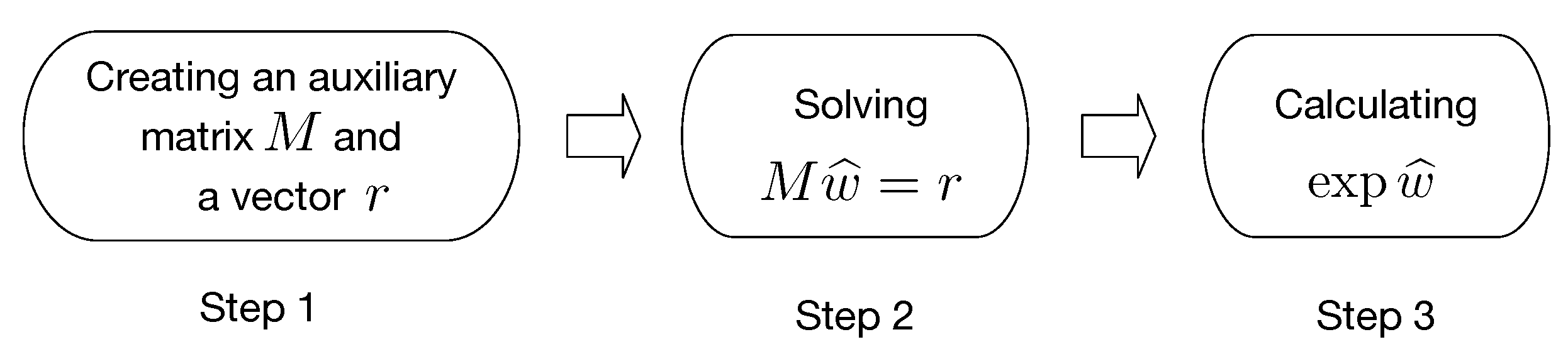
4. Idea of the Geometric Mean Method for Incomplete PC Matrices

Following Harker’s method [30], the proposed solution assumes that C is irreducible ($T_C$ is connected) and the optimal completion of the incomplete PC matrix C is $C^{*}=[c_{ij}^{*}]$ (3). Hence, every missing $c_{ij}=?$ in C is replaced by the ratio $w(a_i)/w(a_j)$ in $C^{*}$. However, unlike in [30], $C^{*}$ is the subject of the GMM. Then, let us calculate the geometric mean of rows for $C^{*}$; i.e.,

$${\left(\prod _{j=1}^n{c}_{ij}^{*}\right)}^{1/n}=w(a_i)\mathit{for}i=1,\dots ,n.$$

(10)

Using the logarithmic transformation on both sides, we get

$$\frac{1}{n}ln\prod _{j=1}^n{c}_{ij}^{*}=lnw(a_i)\mathit{for}i=1,\dots ,n,$$

which is equivalent to

$$\sum _{j=1}^{n}ln{c}_{ij}^{*}=nlnw(a_i)\mathit{for}i=1,\dots ,n.$$

Let us split the left side of the equation into two parts—one for the missing values in C and the other for the existing elements.

$$\sum _{\begin{array}{c}j=1\\ c_{ij}\ne ?\end{array}}^{n}ln{c}_{ij}^{*}+\sum _{\begin{array}{c}j=1\\ c_{ij}=?\end{array}}^{n}ln\frac{w(a_i)}{w(a_j)}=nlnw(a_i)\mathit{for}i=1,\dots ,n.$$

Therefore,

$$\sum _{\begin{array}{c}j=1\\ c_{ij}\ne ?\end{array}}^{n}ln{c}_{ij}-\sum _{\begin{array}{c}j=1\\ c_{ij}=?\end{array}}^{n}lnw(a_j)=nlnw(a_i)-\sum _{\begin{array}{c}j=1\\ c_{ij}=?\end{array}}^{n}lnw(a_i)\mathit{for}i=1,\dots ,n.$$

Let us denote the number of missing elements in the i-th row of C as $S_i={\sum }_{\begin{array}{c}j=1\\ c_{ij}=?\end{array}}^{n}1$. Then,

$$(n-S_i)lnw(a_i)+\sum _{\begin{array}{c}j=1\\ c_{ij}=?\end{array}}^{n}lnw(a_j)=\sum _{\begin{array}{c}j=1\\ c_{ij}\ne ?\end{array}}^{n}ln{c}_{ij}\mathit{for}i=1,\dots ,n.$$

For convenience, let us write $lnw(a_i)=\widehat{w}(a_i)$ and $ln{c}_{ij}={\widehat{c}}_{ij}$. Thus, the above equation system obtains the form

$$(n-S_i)\widehat{w}(a_i)+\sum _{\begin{array}{c}j=1\\ c_{ij}=?\end{array}}^n\widehat{w}(a_j)+\sum _{\begin{array}{c}j=1\\ c_{ij}\ne ?\end{array}}^{n}0=\sum _{\begin{array}{c}j=1\\ c_{ij}\ne ?\end{array}}^{n}ln{c}_{ij}\mathit{for}i=1,\dots ,n.$$

It can be written in the matrix form as

$$M\widehat{w}=r,$$

(11)

where

$$\widehat{w}=\left(\begin{array}{c}\widehat{w}(a_1)\\ ⋮\\ ⋮\\ \widehat{w}(a_n)\end{array}\right),r\stackrel{\mathit{df}}{=}\left(\begin{array}{c}\sum _{\begin{array}{c}j=1\\ c_{1j}\ne ?\end{array}}^{n}ln{c}_{1j}\\ ⋮\\ ⋮\\ \sum _{\begin{array}{c}j=1\\ c_{nj}\ne ?\end{array}}^{n}ln{c}_{nj}\end{array}\right),$$

(12)

and $M=[m_{ij}]$ is such that

$$m_{ij}\stackrel{\mathit{df}}{=}\left\{\begin{array}{cc}n-S_i\hfill & \mathrm{if}i=j\hfill \\ 0\hfill & \mathrm{if}i\ne j\mathrm{and}{c}_{ij}\ne ?\hfill \\ 1\hfill & \mathrm{if}i\ne j\mathrm{and}{c}_{ij}=?\hfill \end{array}\right..$$

(13)

By solving (11) we obtain the auxiliary vector $\widehat{w}$ providing us the solution of the primary problem (10); i.e.,

$$w=\left(\begin{array}{c}{e}^{\widehat{w}(a_1)}\\ ⋮\\ ⋮\\ e^{\widehat{w}(a_n)}\end{array}\right).$$

(14)

Of course, w can be the subject of scaling, so as the final ranking we may adopt $\alpha w$ where $\alpha ={\left({\sum }_{i=1}^n{e}^{\widehat{w}(a_i)}\right)}^{-1}$. As will be shown in Section 6.1 M is nonsingular, hence, (11) and, as follows, (10), always have a unique solution.

Summing up, the above procedure comes down to the following three steps:

• Constructing the auxiliary matrix M as defined in (13) and the constant term vector (12).
• Solving the linear equation system (11).
• Applying the exponential transformation to each of the elements of the vector obtained in the previous step and getting the final ranking vector (14).

The diagram of the calculation process is presented in Figure 1.

5. Illustrative Example

The editors of the automotive magazine decided to compare $a_1,\dots ,a_4$ four cars, concerning the comfort of driving. Due to time and cost constraints, only three direct car comparisons were performed: $a_1$ vs. $a_4$, $a_2$ vs. $a_3$, and $a_3$ vs. $a_4$. The results of comparisons have been denoted as $c_{14}=2,c_{23}=3,$ and $c_{34}=2$. The remaining undefined comparisons $c_{ij}$ were substituted by the ratios in form $w(a_i)/w(a_j)$.

Let us consider the incomplete PC matrix $C^{*}$ formed as a result of the journal’s analysis

$$C^{*}=\left(\begin{array}{cccc}1& \frac{w(a_1)}{w(a_2)}& \frac{w(a_1)}{w(a_3)}& c_{14}\\ \frac{w(a_2)}{w(a_1)}& 1& c_{23}& \frac{w(a_2)}{w(a_4)}\\ \frac{w(a_3)}{w(a_1)}& c_{32}& 1& c_{34}\\ c_{41}& \frac{w(a_4)}{w(a_2)}& c_{43}& 1\end{array}\right).$$

It corresponds to the following equation system:

$$\begin{array}{ccc}{\left(1·\frac{w(a_1)}{w(a_2)}·\frac{w(a_1)}{w(a_3)}·c_{14}\right)}^{1/4}& =& w(a_1)\\ {\left(\frac{w(a_2)}{w(a_1)}·1·c_{23}·\frac{w(a_2)}{w(a_4)}\right)}^{1/4}& =& w(a_2)\\ {\left(\frac{w(a_3)}{w(a_1)}·c_{32}·1·c_{34}\right)}^{1/4}& =& w(a_3)\\ {\left(c_{41}·\frac{w(a_4)}{w(a_2)}·c_{43}·1\right)}^{1/4}& =& w(a_4)\end{array}.$$

To solve it, let us raise both sides to the fourth power,

$$\begin{array}{ccc}1·\frac{w(a_1)}{w(a_2)}·\frac{w(a_1)}{w(a_3)}·c_{14}& =& w^4(a_1)\\ \frac{w(a_2)}{w(a_1)}·1·c_{23}·\frac{w(a_2)}{w(a_4)}& =& w^4(a_2)\\ \frac{w(a_3)}{w(a_1)}·c_{32}·1·c_{34}& =& w^4(a_3)\\ c_{41}·\frac{w(a_4)}{w(a_2)}·c_{43}·1& =& w^4(a_4)\end{array},$$

and apply logarithm transformation to both sides. Then, we obtain

$$\begin{array}{ccc}0-lnw(a_2)-lnw(a_3)+ln{c}_{14}& =& 2lnw(a_1)\\ -lnw(a_1)+0+ln{c}_{23}-lnw(a_4)& =& 2lnw(a_2)\\ -lnw(a_1)+ln{c}_{32}+0+ln{c}_{34}& =& 3lnw(a_3)\\ ln{c}_{41}-lnw(a_2)+ln{c}_{43}+0& =& 3lnw(a_4)\end{array}.$$

(15)

The above (15) can be written as the following linear equation system

$$\begin{array}{ccc}2lnw(a_1)+lnw(a_2)+lnw(a_3)+0& =& ln{c}_{14}\\ lnw(a_1)+2lnw(a_2)+0+lnw(a_4)& =& ln{c}_{23}\\ lnw(a_1)+0+3lnw(a_3)+0& =& +ln{c}_{32}+ln{c}_{34}\\ 0+lnw(a_2)+0+3lnw(a_4)& =& +ln{c}_{41}+ln{c}_{43}\end{array}.$$

Hence, the above equation system can be written down in the matrix form

$$M\widehat{w}=\widehat{c},$$

where the auxiliary matrix M is given as

$$M=\left(\begin{array}{cccc}2& 1& 1& 0\\ 1& 2& 0& 1\\ 1& 0& 3& 0\\ 0& 1& 0& 3\end{array}\right),$$

and the constant term vector $\widehat{c}$ and the vector $\widehat{w}$ are as follows:

$$\widehat{c}=\left(\begin{array}{c}{\widehat{c}}_{14}\\ {\widehat{c}}_{23}\\ {\widehat{c}}_{32}+{\widehat{c}}_{34}\\ {\widehat{c}}_{41}+{\widehat{c}}_{43}\end{array}\right),\widehat{w}=\left(\begin{array}{c}\widehat{w}(a_1)\\ \widehat{w}(a_2)\\ \widehat{w}(a_3)\\ \widehat{w}(a_4)\end{array}\right).$$

Since the matrix M is non-singular, we may compute the auxiliary vector:

$$\widehat{w}=\left(\begin{array}{c}\frac{15{\widehat{c}}_{14}-9{\widehat{c}}_{23}-5{\widehat{c}}_{32}-5{\widehat{c}}_{34}+3{\widehat{c}}_{41}+3{\widehat{c}}_{43}}{16}\\ \frac{-9{\widehat{c}}_{14}+15{\widehat{c}}_{23}+3{\widehat{c}}_{32}+3{\widehat{c}}_{34}-5{\widehat{c}}_{41}-5{\widehat{c}}_{43}}{16}\\ \frac{-5{\widehat{c}}_{14}+3{\widehat{c}}_{23}+7{\widehat{c}}_{32}+7{\widehat{c}}_{34}-{\widehat{c}}_{41}-{\widehat{c}}_{43}}{16}\\ \frac{3{\widehat{c}}_{14}-5{\widehat{c}}_{23}-{\widehat{c}}_{32}-{\widehat{c}}_{34}+7{\widehat{c}}_{41}+7{\widehat{c}}_{43}}{16}\end{array}\right).$$

Finally, after exponential transformation, we obtain the unscaled ranking vector:

$$w=\left(\begin{array}{c}exp\left\{(15{\widehat{c}}_{14}-9{\widehat{c}}_{23}-5{\widehat{c}}_{32}-5{\widehat{c}}_{34}+3{\widehat{c}}_{41}+3{\widehat{c}}_{43})/16\right\}\\ exp\left\{(-9{\widehat{c}}_{14}+15{\widehat{c}}_{23}+3{\widehat{c}}_{32}+3{\widehat{c}}_{34}-5{\widehat{c}}_{41}-5{\widehat{c}}_{43})/16\right\}\\ exp\left\{(-5{\widehat{c}}_{14}+3{\widehat{c}}_{23}+7{\widehat{c}}_{32}+7{\widehat{c}}_{34}-{\widehat{c}}_{41}-{\widehat{c}}_{43})/16\right\}\\ exp\left\{(3{\widehat{c}}_{14}-5{\widehat{c}}_{23}-{\widehat{c}}_{32}-{\widehat{c}}_{34}+7{\widehat{c}}_{41}+7{\widehat{c}}_{43})/16\right\}\end{array}\right).$$

Of course, for specific values, e.g., $c_{14}=c_{34}=2$ and $c_{23}=3$ ($c_{41}=c_{43}=1/2$ and $c_{32}=1/3$), it is easy to compute that $w={[0.18,0.54,0.18,0.09]}^T$. Thus, in this particular case the car $a_2$ is the most comfortable alternative; then ex aequo cars $a_1$ and $a_3$; and the least comfortable car is $a_4$.

6. Properties of the Method

6.1. Existence of a Solution

One may observe that for the fixed incomplete and irreducible PC matrix C, the auxiliary matrix M (13) can be written as:

$$M=L(T_C)+J_n,$$

where $L(T_C)$ is the Laplacian matrix of $T_C$, and $J_n$ is the $n\times n$ matrix, each of whose entries is 1. Proof of the fact that M is non-singular has been provided by Kaiser and Serlin [51] (p. 426). The K matrix in their work is identical to M.

6.2. Optimality

The GM method [50] is considered as optimal since it minimizes the logarithmic least squares (LLS) condition $S(C)$ (6) for some (complete) PC matrix C. It is natural to assume that the LLS condition for an incomplete PC matrix has to be limited to the existing entries. Hence, the LLS condition for the incomplete PC matrices $S^{*}(C)$ (7) has been formulated in a way that the missing values $c_{ij}=?$ are not taken into account [32,33,52].

The proposed method in Section 4 is, in fact, the GM method applied to the completed matrix $C^{*}$. Therefore, due to Crawford’s theorem, the vector w obtained as the solution of (10) minimizes $S(C^{*})$, where

$$S(C^{*})=\sum _{i,j=1}^n{\left(log{c}_{ij}^{*}-log\frac{w(a_i)}{w(a_j)}\right)}^2.$$

Due to the missing values in C, we may rewrite the above equation as

$$S(C^{*})=\sum _{\begin{array}{c}i,j=1\\ c_{ij}\ne ?\end{array}}^n{\left(log{c}_{ij}-log\frac{w(a_i)}{w(a_j)}\right)}^2+\sum _{\begin{array}{c}i,j=1\\ c_{ij}=?\end{array}}^n{\left(log\frac{w(a_i)}{w(a_j)}-log\frac{w(a_i)}{w(a_j)}\right)}^2.$$

Hence,

$$S(C^{*})=\sum _{\begin{array}{c}i,j=1\\ c_{ij}\ne ?\end{array}}^n{\left(log{c}_{ij}-log\frac{w(a_i)}{w(a_j)}\right)}^2,$$

Thus, $S^{*}(C)=S(C^{*})$, so the proposed method, Section 4, minimizes $S^{*}(C)$. Hence, it is optimal. This also means that it is equivalent to the ILLSM as defined in [31,32].

7. Summary

In this work, the GMM for incomplete PC matrices has been presented. It can be viewed as a twin approach to the LLSM for an incomplete PCM, as both methods are equivalent. They lead to the same result and are based on the same assumption that the ratio $w(a_i)/w(a_j)$ substitutes the missing elements in $C=[c_{ij}]$.They differ in the starting point for considerations. In line with its name IGMM starts from constructing geometric means of PCM rows. Simultaneously, ILLSM shortens this reasoning by proposing to start deliberations with a logarithmic criterion (6, 7). Both methods lead to a system of linear equations indispensable to calculating the results. However, the two systems of equations are slightly different. In ILLSM, the matrix of a system $L(T_C)$ is the Laplacian matrix of the PCM C, while in IGMM, the system’s matrix is the Laplacian matrix plus matrix of ones, i.e., $L(T_C)+J_n$. In both cases, the equations are easy to solve.

Since both the ILLSM and IGMM methods are so similar, is it worth distinguishing between them? We believe that it is worth it, just as there are in the literature twin parallel LLSM and GMM. In particular, since GMM appears to be more widespread than LLSM due to the simplicity of calculating the geometric mean, IGMM may likewise be more recognizable than ILLSM. Perhaps the definition of IGMM will also contribute to greater recognition of ILLSM among practitioners dealing with multi-criteria decision-making methods.

References

1. Colomer, J.M. Ramon Llull: From ‘Ars electionis’ to social choice theory. Soc. Choice Welf. 2011, 40, 317–328. [Google Scholar] [CrossRef]
2. Condorcet, M. Essay on the Application of Analysis to the Probability of Majority Decisions; Imprimerie Royale: Paris, France, 1785. [Google Scholar]
3. Thurstone, L.L. A Law of Comparative Judgment, reprint of an original work published in 1927. Psychol. Rev. 1994, 101, 266–270. [Google Scholar] [CrossRef]
4. Copeland, A.H. A “reasonable” social welfare function. In Seminar on Applications of Mathematics to Social Sciences; University of Michigan: Ann Arbor, MI, USA, 1951. [Google Scholar]
5. Saaty, T.L. A scaling method for priorities in hierarchical structures. J. Math. Psychol. 1977, 15, 234–281. [Google Scholar] [CrossRef]
6. Doumpos, M.; Figueira, J.R. A multicriteria outranking approach for modeling corporate credit ratings: An application of the ELECTRE TRI-NC method. Omega 2019, 82, 166–180. [Google Scholar] [CrossRef]
7. Brans, J.; Mareschal, B. PROMETHEE Methods. In Multiple Criteria Decision Analysis: State of the Art Surveys; Figueira, J., Greco, S., Ehrgott, M., Eds.; Springer: London, UK, 2005; pp. 163–196. [Google Scholar]
8. Qi, X.; Yu, X.; Wang, L.; Liao, X.; Zhang, S. PROMETHEE for prioritized criteria. Soft Comput. 2019, 23, 11419–11432. [Google Scholar] [CrossRef]
9. Jamshidi, A.; Jamshidi, F.; Ait-Kadi, D.; Ramudhin, A. A review of priority criteria and decision-making methods applied in selection of sustainable city logistics initiatives and collaboration partners. Int. J. Prod. Res. 2019, 57, 5175–5193. [Google Scholar] [CrossRef] [Green Version]
10. Bana e Costa, C.; De Corte, J.M.; Vansnick, J. On the Mathematical Foundation of MACBETH. In Multiple Criteria Decision Analysis: State of the Art Surveys; Figueira, J., Greco, S., Ehrgott, M., Eds.; Springer: London, UK, 2005; pp. 409–443. [Google Scholar]
11. Cinelli, M.; Kadziński, M.; Gonzalez, M.; Słowiński, R. How to support the application of multiple criteria decision analysis? Let us start with a comprehensive taxonomy. Omega 2020, 96, 102261. [Google Scholar] [CrossRef]
12. Kułakowski, K.; Grobler-Dębska, K.; Wąs, J. Heuristic rating estimation: Geometric approach. J. Glob. Optim. 2015, 62, 529–543. [Google Scholar] [CrossRef] [Green Version]
13. Liang, F.; Brunelli, M.; Rezaei, J. Consistency issues in the best worst method: Measurements and thresholds. Omega 2019, 96, 102175. [Google Scholar] [CrossRef]
14. Mohammadi, M.; Rezaei, J. Bayesian best-worst method: A probabilistic group decision making model. Omega 2020, 96, 102075. [Google Scholar] [CrossRef]
15. Greco, S.; Matarazzo, B.; Słowiński, R. Dominance-Based Rough Set Approach to Preference Learning from Pairwise Comparisons in Case of Decision under Uncertainty. In Computational Intelligence for Knowledge-Based Systems Design; Hüllermeier, E., Kruse, R., Hoffmann, F., Eds.; Lecture Notes in Computer Science; Springer: Berlin/Heidelberg, Germany, 2010; Volume 6178, pp. 584–594. [Google Scholar]
16. Ramík, J. Strong reciprocity and strong consistency in pairwise comparison matrix with fuzzy elements. Fuzzy Optim. Decis. Mak. 2018, 17, 337–355. [Google Scholar] [CrossRef]
17. Domínguez, S.; Carnero, M.C. Fuzzy multicriteria modelling of decision making in the renewal of healthcare technologies. Mathematics 2020, 8, 944. [Google Scholar] [CrossRef]
18. Cavallo, B.; Brunelli, M. A general unified framework for interval pairwise comparison matrices. Int. J. Approx. Reason. 2018, 93, 178–198. [Google Scholar] [CrossRef] [Green Version]
19. Kułakowski, K.; Mazurek, J.; Ramík, J.; Soltys, M. When is the condition of order preservation met? Eur. J. Oper. Res. 2019, 277, 248–254. [Google Scholar] [CrossRef] [Green Version]
20. Wajch, E. From pairwise comparisons to consistency with respect to a group operation and Koczkodaj’s metric. Int. J. Approx. Reason. 2019, 106, 51–62. [Google Scholar] [CrossRef]
21. Janicki, R.; Zhai, Y. On a pairwise comparison-based consistent non-numerical ranking. Log. J. IGPL 2012, 20, 667–676. [Google Scholar] [CrossRef]
22. Brunelli, M. A survey of inconsistency indices for pairwise comparisons. Int. J. Gen. Syst. 2018, 47, 751–771. [Google Scholar] [CrossRef]
23. Bozóki, S.; Fülöp, J.; Poesz, A. On reducing inconsistency of pairwise comparison matrices below an acceptance threshold. Cent. Eur. J. Oper. Res. 2015, 23, 849–866. [Google Scholar] [CrossRef] [Green Version]
24. Kułakowski, K.; Szybowski, J. The New Triad based Inconsistency Indices for Pairwise Comparisons. Procedia Comput. Sci. 2014, 35, 1132–1137. [Google Scholar] [CrossRef] [Green Version]
25. Kułakowski, K. Inconsistency in the ordinal pairwise comparisons method with and without ties. Eur. J. Oper. Res. 2018, 270, 314–327. [Google Scholar] [CrossRef] [Green Version]
26. Iida, Y. Ordinality consistency test about items and notation of a pairwise comparison matrix in AHP. In Proceedings of the International Symposium on the Analytic Hierarchy Process, University of Pittsburgh, Pittsburgh, PA, USA, 1 August 2009. [Google Scholar]
27. Bozóki, S. Inefficient weights from pairwise comparison matrices with arbitrarily small inconsistency. Optimization 2014, 63, 1893–1901. [Google Scholar] [CrossRef] [Green Version]
28. Kułakowski, K. On the Properties of the Priority Deriving Procedure in the Pairwise Comparisons Method. Fundam. Inf. 2015, 139, 403–419. [Google Scholar] [CrossRef] [Green Version]
29. Koczkodaj, W.W.; Magnot, J.P.; Mazurek, J.; Peters, J.F.; Rakhshani, H.; Soltys, M.; Strzałka, D.; Szybowski, J.; Tozzi, A. On normalization of inconsistency indicators in pairwise comparisons. Int. J. Approx. Reason. 2017, 86, 73–79. [Google Scholar] [CrossRef] [Green Version]
30. Harker, P.T. Alternative modes of questioning in the analytic hierarchy process. Math. Model. 1987, 9, 353–360. [Google Scholar] [CrossRef] [Green Version]
31. Tone, K. Logarithmic Least Squares Method for Incomplete Pairwise Comparisons in the Analytic Hierarchy Process; Technical Report 94-B-2; Institute for Policy Science Research, Saitama University: Saitama, Japan, 1993. [Google Scholar]
32. Bozóki, S.; Fülöp, J.; Rónyai, L. On optimal completion of incomplete pairwise comparison matrices. Math. Comput. Model. 2010, 52, 318–333. [Google Scholar] [CrossRef] [Green Version]
33. Bozóki, S.; Tsyganok, V. The (logarithmic) least squares optimality of the arithmetic (geometric) mean of weight vectors calculated from all spanning trees for incomplete additive (multiplicative) pairwise comparison matrices. Int. J. Gen. Syst. 2019, 48, 362–381. [Google Scholar] [CrossRef]
34. Tsyganok, V. Combinatorial method of pairwise comparisons with feedback, data Recording. Storage Process. 2000, 2, 92–102. [Google Scholar]
35. Tsyganok, V. Investigation of the aggregation effectiveness of expert estimates obtained by the pairwise comparison method. Math. Comput. Model. 2010, 52, 538–544. [Google Scholar] [CrossRef]
36. Siraj, S.; Mikhailov, L.; Keane, J.A. Enumerating all spanning trees for pairwise comparisons. Comput. Oper. Res. 2012, 39, 191–199. [Google Scholar] [CrossRef]
37. Lundy, M.; Siraj, S.; Greco, S. The mathematical equivalence of the “spanning tree” and row geometric mean preference vectors and its implications for preference analysis. Eur. J. Oper. Res. 2017, 257, 197–208. [Google Scholar] [CrossRef] [Green Version]
38. Koczkodaj, W.W.; Herman, M.W.; Orlowski, M. Managing Null Entries in Pairwise Comparisons. Knowl. Inf. Syst. 2013, 1, 119–125. [Google Scholar] [CrossRef] [Green Version]
39. Koczkodaj, W.W.; Szybowski, J. Pairwise comparisons simplified. Appl. Math. Comput. 2015, 253, 387–394. [Google Scholar] [CrossRef] [Green Version]
40. Ergu, D.; Kou, G.; Peng, Y.; Zhang, M. Estimating the missing values for the incomplete decision matrix and consistency optimization in emergency management. Appl. Math. Model. 2016, 40, 254–267. [Google Scholar] [CrossRef]
41. Alonso, S.; Chiclana, F.; Herrera, F.; Viedma-Herrera, E.; Alcalá-Fdez, J.; Porcel, C. A consistency-based procedure to estimate missing pairwise preference values. Int. J. Intell. Syst. 2008, 23, 155–175. [Google Scholar] [CrossRef]
42. Jandová, V.; Krejci, J.; Stoklasa, J.; Fedrizzi, M. Computing Interval Weights for Incomplete Pairwise-Comparison Matrices of Large Dimension—A Weak-Consistency-Based Approach. Fuzzy Syst. IEEE Trans. 2017, 25, 1714–1728. [Google Scholar] [CrossRef]
43. Zhou, X.; Hu, Y.; Deng, Y.; Chan, F.T.; Ishizaka, A. A DEMATEL-based completion method for incomplete pairwise comparison matrix in AHP. Ann. Oper. Res. 2018, 271, 1045–1066. [Google Scholar] [CrossRef] [Green Version]
44. Alrasheedi, M.A. Incomplete pairwise comparative judgments: Recent developments and a proposed method. Decis. Sci. Lett. 2019, 8, 261–274. [Google Scholar] [CrossRef]
45. Oliva, G.; Setola, R.; Scala, A. Sparse and distributed Analytic Hierarchy Process. Automatica 2017, 85, 211–220. [Google Scholar] [CrossRef]
46. Kułakowski, K.; Talaga, D. Inconsistency indices for incomplete pairwise comparisons matrices. Int. J. Gen. Syst. 2020, 49, 174–200. [Google Scholar] [CrossRef] [Green Version]
47. Gavalec, M.; Ramik, J.; Zimmermann, K. Decision Making and Optimization: Special Matrices and Their Applications in Economics and Management; Number 677 in Lecture Notes in Economics and Mathematical Systems; Springer: Berlin/Heidelberg, Germany, 2014. [Google Scholar]
48. Quarteroni, A.; Sacco, R.; Saleri, F. Numerical Mathematics; Springer: Berlin/Heidelberg, Germany, 2000. [Google Scholar]
49. Cormen, T.H.; Leiserson, C.E.; Rivest, R.L.; Stein, C. Introduction to Algorithms, 3rd ed.; MIT Press: Cambridge, MA, USA, 2009. [Google Scholar]
50. Crawford, G.; Williams, C. The Analysis of Subjective Judgment Matrices; Technical Report R-2572-1-AF; The Rand Corporation: Santa Monica, CA, USA, 1985. [Google Scholar]
51. Kaiser, H.F.; Serlin, R.C. Contributions to the method of paired comparisons. Appl. Psychol. Meas. 1978, 2, 423–432. [Google Scholar] [CrossRef] [Green Version]
52. Kwiesielewicz, M. The logarithmic least squares and the generalized pseudoinverse in estimating ratios. Eur. J. Oper. Res. 1996, 93, 611–619. [Google Scholar] [CrossRef]
Figure 1. Scheme of the IGMM.
Mathematics 08 01873 g001
Publisher’s Note: MDPI stays neutral with regard to jurisdictional claims in published maps and institutional affiliations.