A Dynamic Duopoly Model: When a Firm Shares the Market with Certain Profit

Abstract

The current paper analyzes a competition of the Cournot duopoly game whose players (firms) are heterogeneous in a market with isoelastic demand functions and linear costs. The first firm adopts a rationally-based gradient mechanism while the second one chooses to share the market with certain profit in order to update its production. It trades off between profit and market share maximization. The equilibrium point of the proposed game is calculated and its stability conditions are investigated. Our studies show that the equilibrium point becomes unstable through period doubling and Neimark–Sacker bifurcation. Furthermore, the map describing the proposed game is nonlinear and noninvertible which lead to several stable attractors. As in literature, we have provided an analytical investigation of the map’s basins of attraction that includes lobes regions.

1. Introduction

The history of literature has recorded several studies on the dynamic behavior of Cournot duopoly games. Such games are usually represented by discrete dynamical systems whose dynamic characteristics are of great important to mathematicians and economists. Studying those dynamics in a global way has given more insights about the time evolution of maps describing such games in the future. In duopoly games, there are only two competing firms, and due to the lack of market information, those competitors adopt different mechanisms in order to update their outputs. These mechanisms have included a gradient-based approach such as bounded rationality, and other mechanisms such as local monopolistic approximation (LMA), adaptive mechanism and recently profit-sharing mechanism.

Firms choosing the bounded rationality approach to play within the market do not have to know complete information about demand and cost functions. They require only an estimation of their marginal profits. In particular, this approach has been thoroughly used in many works and has recently gained considerable popularity in literature. For instance, a Cournot duopoly game has been introduced and discussed using the bounded rationality mechanism in [1]. This mechanism has also been adopted in [2] to study a chaotic congestion game. The stability of equilibrium points of an R&D competition has been analyzed for a model of duopoly based on the bounded rationality mechanism in [3]. The influences of cost uncertainty of a duopoly game based on a concave demand function and derived from bounded rationality have been investigated in [4]. The bounded rationality mechanism has been used to construct and study a piecewise smooth map representing a remanufacturing duopoly game in [5]. In [6], the mechanism has been adopted to investigate the complex characteristics of a heterogeneous triopoly game. Based on the rationality mechanism, some complex dynamic characteristics such as bifurcation, multistability and intermittent chaos of a two-stage Cournot game have been analyzed in [7]. The constant elasticity of substitution (CES) production utility function has been recalled with the bounded rationality approach in [8] to investigate complex dynamic characteristics of an oligopoly game. In [9], a duopoly Stackelberg game and its dynamic characteristics have been formulated and studied based on the rationality mechanism. A duopoly game with price competition based on bounded rationality applied to relative profit has been introduced and discussed in [10]. For more information about this mechanism and others, readers are advised to see more works in literature ([11,12,13,14,15,16]).

Heterogeneous mechanisms have been studied in several works in literature. For instance, Leonard et al. [17], Tramontana [18], Agiza and Elsadany [19,20] and others in literature have concerned duopoly games whose players adopted gradient-like and LMA mechanisms. In the current manuscript, we consider a duopoly game that belongs to these works and whose players adopt the gradient-like and a certain profit mechanism. The certain profit mechanism is a trade-off between profit and market share maximization. It is worth highlighting that this mechanism has been used in [21,22] but the analysis of the model based on that mechanism was improper as in those references the authors had to handle their model as a piecewise smooth map. Proper usage of that mechanism has been published in [5]. Our economic structure in this paper is similar to those introduced in [18,23] in which an isoelastic demand function and linear costs have been assumed. In particular, our model describing the duopoly game differs from those in the decisional mechanism adopted by the second firm. The mechanism adopted by the second firm in our model is more general than those in [18] and is more complicated than the one used by Cavalli et al. in [23]. The global analysis carried out in this paper shows the destabilization of the equilibrium point due to two different routes to chaos. These routes are formed because of the existence of period-doubling and Neimark–Sacker bifurcations and a mixed scenario of them. The nonlinearity and noninvertibility of the game’s map show several stable attractors (multi-stability). The phase plane of the game’s map is quite complicated and this is because our investigations detect particular shapes known as lobes in the basins of attraction for some attractive sets.

After the above introduction, we can now summarize the current paper. In Section 2, we introduce the nonlinear map that describes the game at hand. In Section 3, we calculate the map’s fixed points and study their conditions of stability. A rich local and global analysis of the complex dynamic characteristics of the map such as bifurcations, period cycles, chaotic attractors and closed invariant sets is given in Section 4. In Section 5, we study another important aspect of the map that is noninvertibility and critical curves. In the last section, we give the conclusion.

2. The Model

We consider in this paper a duopoly game between two firms, firm 1 and firm 2. The demand productions of each firm are denoted by $x_1$ and $x_2$, respectively. We recall the isoelastic demand function derived from the Cobb–Douglas utility function [24].

$$p=\frac{1}{Q}=\frac{1}{x_1+x_2},$$

(1)

where Q denotes the total supply. Suppose that both firms adopt linear cost functions given by,

$$C_i\left(x_i\right)=c_i{x}_i,i=1,2,$$

(2)

and $\frac{\partial C_i}{\partial x_i}=c_i$ refers to the marginal cost and is greater than zero. The profit of each firm becomes,

$${\pi }_i=\frac{x_i}{{\sum }_{i=1}^2{x}_i}-c_i{x}_i,i=1,2,$$

(3)

and then the marginal profits take the following form,

$$\begin{array}{c}\frac{\partial {\pi }_1}{\partial x_1}=\frac{x_2}{{\left({\sum }_{i=1}^2{x}_i\right)}^2}-c_1,\hfill \\ \frac{\partial {\pi }_2}{\partial x_2}=\frac{x_1}{{\left({\sum }_{i=1}^2{x}_i\right)}^2}-c_2.\hfill \end{array}$$

(4)

Now, we assume heterogeneous firms on which the two firms use different mechanisms in order to update their outputs each period of time. The first firm adopts the so-called bounded rationality mechanism introduced in [25]. So the first firm will update its production each time period according to the following,

$$x_{1,t+1}=x_{1,t}+\alpha x_{1,t}\frac{\partial {\pi }_1}{\partial x_{1,t}},$$

(5)

where $\alpha$ is a positive parameter named the speed of adjustment parameter. On the other hand, the second firm chooses to share the market with a certain profit in order to update its production. This may be done as follows. If it seeks a complete market share maximization, this gives ${\pi }_2=0$ and then the firm’s optimum output is given by,

$${\overline{x}}_2=\frac{1}{c_2}-x_1.$$

(6)

That is positive provided that $x_1<\frac{1}{c_1}$. However, if it completely seeks profit maximization, its marginal profit will vanish and in that case the optimum output of the firm becomes,

$${\widehat{x}}_2=\sqrt{\frac{x_1}{c_2}}-x_1.$$

(7)

That is also positive provided that $x_1<\frac{1}{c_1}$. So the firm will be traded off between profit and market share according to the following,

$$\begin{array}{c}{\tilde{x}}_2=\omega {\overline{x}}_2+(1-\omega ){\widehat{x}}_2\hfill \\ =\frac{\omega }{c_2}-x_1+(1-\omega )\sqrt{\frac{x_1}{c_2}}\hfill \end{array},$$

(8)

where $\omega \in (0,1)$. When $\omega =0$ the second firm only seeks profit maximization and $\omega =1$ gives only market share maximization. However, the firm is traded off between both, it updates its output each period of time using the following adaptive mechanism.

$$x_{2,t+1}=(1-\beta )x_{2,t}+\beta {\tilde{x}}_{2,t},$$

(9)

where $\beta \in (0,1)$. Such adaptive mechanism shows that the second firm updates its next period output based on some weights between the previous and optimum of the market share. Now, the duopoly game is described by the following 2D nonlinear discrete dynamical system,

$$T(x_1,x_2):\left\{\begin{array}{c}{x}_{1,t+1}=x_{1,t}+\alpha x_{1,t}\left(\frac{x_{2,t}}{{\left({\sum }_{i=1}^2{x}_{i,t}\right)}^2}-c_1\right),\hfill \\ x_{2,t+1}=x_{2,t}+\beta \left(\frac{\omega }{c_2}-x_{1,t}-x_{2,t}+(1-\omega )\sqrt{\frac{x_{1,t}}{c_2}}\right).\hfill \end{array}\right.$$

(10)

It should be noted that the map (10) is not defined at the origin $\left(0,0\right)$. Our proposed model is similar to the models studied in [18,23]. Indeed, our model’s mechanism is similar to both mechanisms adopted by the first firm in those models. The mechanism adopted by the second firm in our model here is more general than the one adopted one by the second firm in [18]. In fact, if we put $\beta =1$ and $\omega =0$ in our model (10) one gets Tramontana’s model discussed in [18]. Regarding the model studied in [23], the second firm uses a different mechanism than ours.

3. The Fixed Points and Stability

In order to get the fixed points of the map (10), we set $x_{1,t+1}=x_{1,t}=x_1^{*}$ and $x_{2,t+1}=x_{2,t}=x_2^{*}$ in (10). This gives the following points,

$$\begin{array}{c}{E}_1=(0,\frac{\omega }{c_2}),\hfill \\ E_2=\left(x_1^{*},x_2^{*}\right),\hfill \end{array}$$

(11)

where,

$$\begin{array}{c}{x}_1^{*}={\left(\frac{(1-\omega )\left(c_2-2c_1\omega \right)+\sqrt{c_2\left[c_2{(1+\omega )}^2-4c_1{\omega }^2\right]}}{2c_2\left[c_2+{(1-\omega )}^2{c}_1\right]}\right)}^2,\hfill \\ x_2^{*}=\frac{c_1}{2c_2}\left(\frac{c_2\left(1+{\omega }^4\right)+\left(1-\omega \right)\left(1+{\omega }^2\right)\sqrt{c_2\left[c_2{(1+\omega )}^2-4c_1{\omega }^2\right]}-2c_1{\omega }^2{\left(1-\omega \right)}^2}{{\left[c_2+{(1-\omega )}^2{c}_1\right]}^2}\right).\hfill \end{array}$$

(12)

The boundary point $E_1$ is considered as a monopoly point as it gives a situation of leaving the market by the first firm and then it becomes dominated only by the second firm. Therefore, we have only the second equation of map (10). It is easy to see that $E_1$ is locally asymptotically stable under the condition $0<\beta <2$. It should be noted that the point $E_2\in {\mathbb{R}}_{+}^2$ under the condition $\frac{c_1}{c_2}<{\left(\frac{1+\omega }{2\omega }\right)}^2$. For the stability of this interior equilibrium point $E_2$, which is the equilibrium of the game, we recall the Jacobian matrix at this point,

$$J_m=\left[\begin{array}{cc}1-\alpha \left(\frac{c_1{(x_1^{*}+x_2^{*})}^3+(x_1^{*}-x_2^{*})x_2^{*}}{{(x_1^{*}+x_2^{*})}^3}\right)& \frac{\alpha x_1^{*}(x_1^{*}-x_2^{*})}{{(x_1^{*}+x_2^{*})}^3}\\ \frac{\beta \left(1-\omega -2\sqrt{c_2{x}_1^{*}}\right)}{2\sqrt{c_2{x}_1^{*}}}& 1-\beta \end{array}\right].$$

(13)

The above matrix has ${\lambda }^2-\tau \lambda +\delta$ as its characteristic equation where $\tau$ and $\delta$ are the trace and determinant of (13). They take the following forms at $E_2$.

$$\begin{array}{c}\tau =2-\beta -\alpha \left(\frac{c_1{(x_1^{*}+x_2^{*})}^3+(x_1^{*}-x_2^{*})x_2^{*}}{{(x_1^{*}+x_2^{*})}^3}\right),\hfill \\ \delta =\frac{\sqrt{c_2}\left[2(1-\beta )(1-\alpha c_1){(x_1^{*}+x_2^{*})}^3+2\alpha (x_1^{*}-x_2^{*})\left(\beta x_1^{*}+(1-\beta )x_2^{*}\right)\right]-\alpha \beta (1-\omega )(x_1^{*}-x_2^{*})}{2\sqrt{c_2}{(x_1^{*}+x_2^{*})}^3}.\hfill \end{array}$$

(14)

Therefore, the stability conditions for $E_2$ are,

$$\begin{array}{c}1-\tau +\delta >0,\hfill \\ 1+\tau +\delta >0,\hfill \\ 1-\delta >0.\hfill \end{array}$$

(15)

The next section gives whether the conditions (15) are satisfied or which types of bifurcations make $E_2$ unstable.

4. Bifurcations

In this section, we analyze the complex dynamic behavior of the map (10). We show that there are two types of bifurcations by which routes to chaos coexist. Those types are the period-doubling and Neimark–Sacker bifurcations. Our analysis begins with assuming the parameter values, $c_1=0.3,c_2=0.9,\omega =0.5$ and $\beta =0.45$. Here, we take $\alpha$ as the bifurcation parameter and keep all the other parameters fixed. We assume the symmetric case of the second firm, which means that $\omega =0.5$ follows an average preference between profit and market share. At this set of values, we have a positive equilibrium point, $E_2=\left(0.6983990501,0.2976105167\right)$. Let us take $\alpha =4$, then the Jacobian matrix (13) becomes,

$$J_m=\left[\begin{array}{cc}-0.6828731121& 1.133152573\\ -0.3081009632& 0.55\end{array}\right],$$

whose eigenvalues are ${\lambda }_1=0.1092581464$ and ${\lambda }_2=-0.2421312585$. They are real and their absolute values lie within the open circle and hence $E_2$ is locally asymptotically stable. In addition, it is easy to see that the conditions of stability (15) are satisfied. The numerical experiments show that $E_2$ is stable for the values of $\alpha \le 5.387$. At $\alpha \approx 5.388$ the period two-cycle is born. 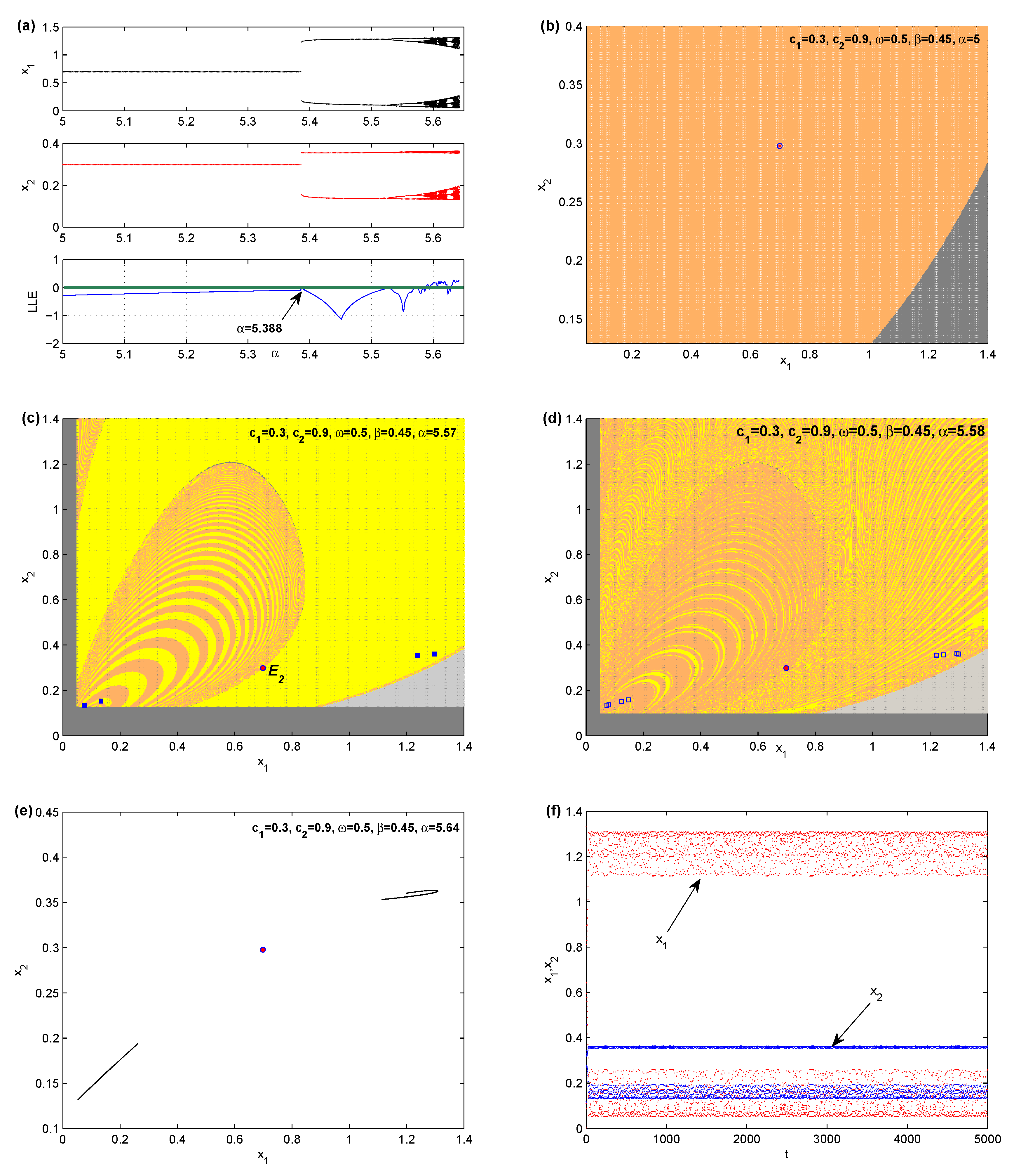Figure 1a presents the kind of bifurcation by which the equilibrium point becomes unstable. It is a period-doubling bifurcation. As one can see, increasing the parameter $\alpha$ gives rise to period 4-cycle, 8-cycle and other higher period cycles, then routes to chaotic behaviors of the map arise around equilibrium point. Globally, at $\alpha =5$ and the other parameter values are kept fixed as previously, we get only the stable equilibrium point. It is plotted with its basin of attraction in Figure 1b, where the grey color denotes divergent and unfeasible trajectories. Increasing $\alpha$ further gives a quite complicated phase plane. The stable period 2-cycle continues to appear as $\alpha$ increases and then the period 4-cycle arises at $\alpha \approx 5.57$. Figure 1c shows the basin of this 4-cycle (represented by squares) with the equilibrium point (represented by circle). The yellow and orange colors characterize the basin of attraction of this cycle. As $\alpha$ increases the basin becomes more complicated. The nonlinearity of map (10) gives a consequence of multistability and hence the basin becomes complicated. Keeping the other parameter values fixed and take $\alpha =5.58$ a stable period 8-cycle and its basin emerged with the equilibrium point in Figure 1d. Higher periodic cycles appear as $\alpha$ increases and then at $\alpha \approx 5.63$ chaotic attractors are born. Figure 1e,f show two-piece chaotic attractors of the map (10) around the equilibrium point and the time series for both variables, respectively.

On the other hand, other routes to chaos are born at the parameter values $c_1=0.15,c_2=0.9,\omega =0.5$ and $\beta =0.95$. It occurs for low values for the cost $c_1$ and high values of both $c_2$ and $\beta$. At this set of values we also have a positive equilibrium point, $E_2=\left(0.8856979217,0.1658689243\right)$. Let us take $\alpha =2.2$, then the Jacobian matrix (13) becomes,

$$J_m=\left[\begin{array}{cc}0.4441051182& 1.206221288\\ -0.6839890304& 0.05\end{array}\right],$$

whose eigenvalues are ${\lambda }_{1,2}=0.247\pm 0.88665i$. They are complex conjugate and their absolute values lie within the open circle and hence $E_2$ is locally asymptotically stable. In addition, it is easy to see that the conditions of stability (15) are satisfied. As $\alpha$ varies a Neimark–Sacker bifurcation takes place. It starts above the value $2.506$, and quasi-periodic motions continue to appear until $\alpha =3.045$ where those motions are replaced by periodic one, specifically a period 9-cycle emerges. In Figure 2a,b, we show Neimark–Sacker bifurcation on varying $\alpha$. Figure 2c depicts the quasi-periodic motion and the stable period 9-cycle at $\alpha =3.044$ and $\alpha =3.045$, respectively. In Figure 2d, we give a consequence of stable spirals due to Neimark–Sacker bifurcation when $\alpha$ takes the values, $2.58,2.60,2.61,2.62$ and the other parameter values are fixed. As $\alpha$ continues to increase, the spiral around the equilibrium point is converted into an invariant attracting closed curve that is given in Figure 2e for different values of $\alpha$. This closed curve implies the coexistence of quasi-periodic motion as reported above. The quasi-periodic motion refers to a predictable macroeconomic behavior of the map’s output. As in [18], the dynamic of the map (10) changes from quasi-periodic motion to a period 9-cycle that has some iterations with negative demand outputs. The basins of attraction of this cycle are quite complicated as shown in Figure 2f, where the grey colors denote the divergent and unfeasible trajectories. It should be noted that all the parameter values are fixed at $c_1=0.15,c_2=0.9,\omega =0.5$ and $\beta =0.95$ in Figure 2. It can be seen from Figure 2a that after Neimark–Sacker bifurcation there are open windows that give rise to periodic, instead of quasi-periodic, cycles. It is obvious that the period 9-cycle is followed by a period 18-cycle that has some negative iteration. It is formed due to period-doubling bifurcation inside the open windows. 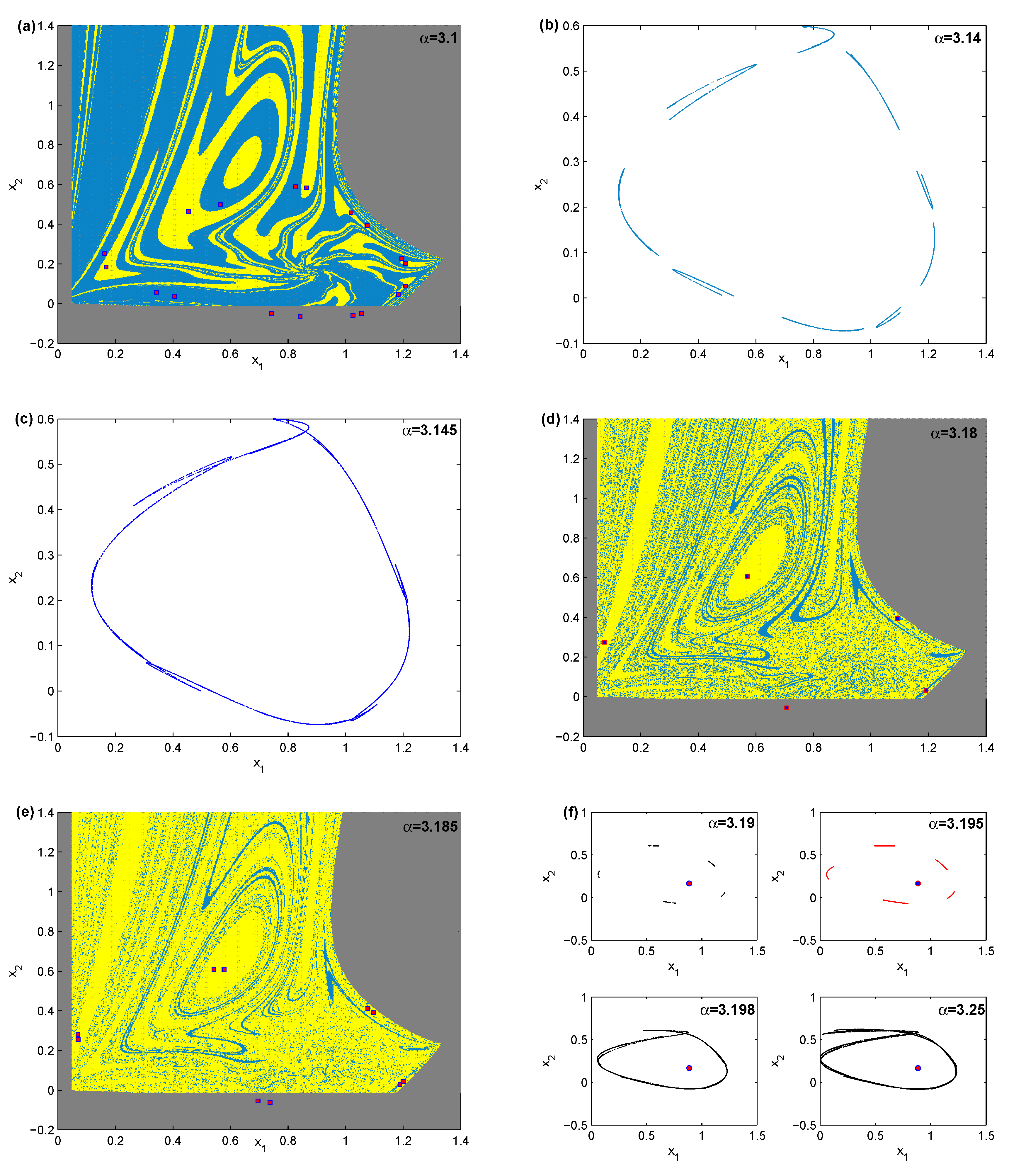Figure 3a shows the basin of the period 18-cycle where the grey colors refer to divergent and unfeasible trajectories. Increasing $\alpha$ to $3.14$, a 9-piece chaotic attractor is born that gathers into one piece chaotic attractor at $\alpha =3.145$ as given in Figure 3b,c, respectively. Increasing $\alpha$ further reports an unconnected 9-piece chaotic attractor which starts gathering to one piece when $\alpha$ approaches $3.145$. This one piece continues to appear and is converted into a period 5-cycle with some negative iterations at $\alpha =3.18$ as shown in Figure 3d. Increasing this parameter further, a period 10-cycle with negative iterations exists in Figure 3e. Finally, any other increase in the bifurcation parameter $\alpha$ makes the map’s dynamics become increasingly chaotic as in Figure 3f.

From the previous discussion, we remark that the main feature of the map (10) is that its dynamic becomes complicated due to two different types of bifurcations. Those types are period-doubling and Neimark–Sacker bifurcation. Because the map has five parameters and the equilibrium point has a complicated expression, it is hard to put a clear form for the stability conditions (15). Instead, we have performed some numerical simulation which has provided some insights about the map’s dynamics. We have observed that the bifurcation parameter $\alpha$ yielded chaotic behavior of the map due to period-doubling bifurcation when we took small values of the first firm’s cost $c_1$, compared with those by the other firm ($c_2$), besides the small value of $\beta$. Indeed, the second equation of (10) contains three important parameters that are $c_2$, $\omega$ and $\beta$. In the previous discussion, we have kept those parameter values fixed and studied the influences of $\alpha$. It shows that the map’s equilibrium point $E_2$ becomes unstable due to Neimark–Sacker bifurcation when $c_1<<c_2$ as shown before. Furthermore, a mixed scenario is detected for the map’s dynamic which is due to the two types of bifurcations. It is observed above that after the Neimark–Sacker bifurcation, there were some periodic windows which lead the map’s dynamics to change from quasi-periodic motion to periodic motion. 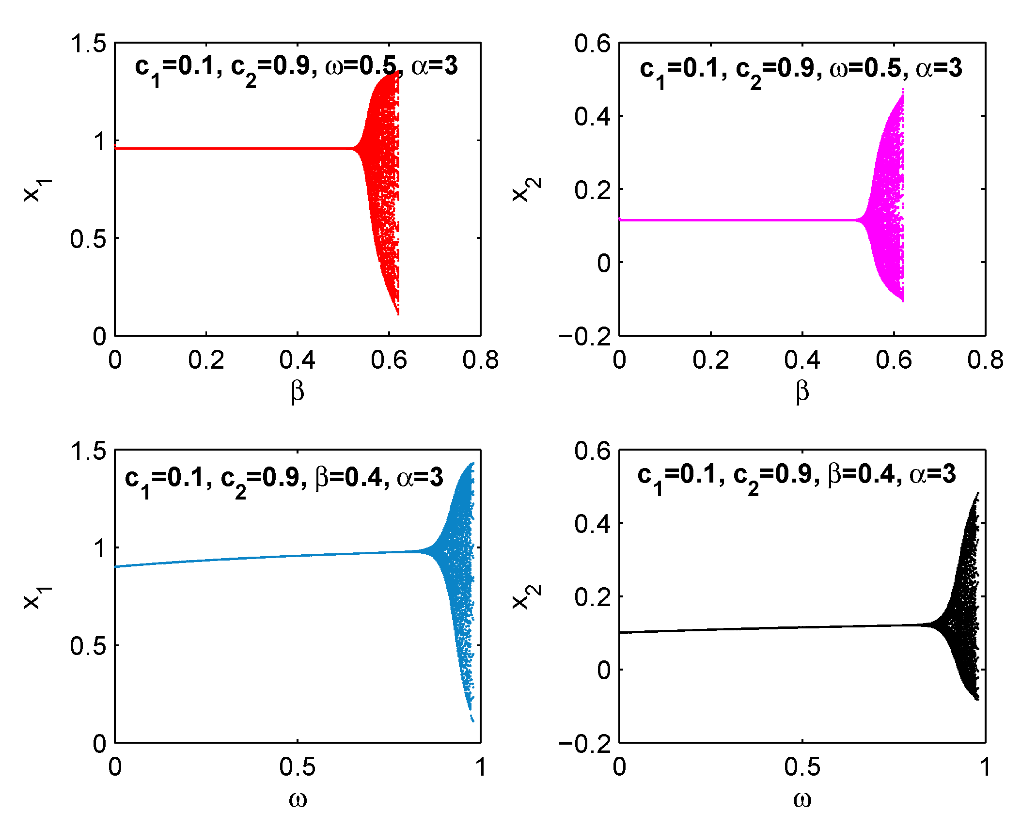We conclude this section by giving the impact of the other parameters $\beta$ and $\omega$ on the map’s dynamics in the following figure. Figure 4 shows that the map’s fixed point becomes unstable because of Neimark–Sacker bifurcation on varying the parameters $\beta$ and $\omega$ keeping the other parameters’ values at $c_1=0.15,c_2=0.9$ and $\alpha =3$. The discussion carried out so far reveals that the map’s dynamic are quite complicated. This is clear from the shape of basins of attraction and the corresponding trajectories obtained above. Therefore, getting more insights into the map’s trajectories lets us take into consideration two important features of the map (10). The first one is that the map is a noninvertible map, as will be discussed in the next section. Secondly, the map has one of its components (the denominator of the first equation in (10)) vanishing at $x_1=-x_2$.

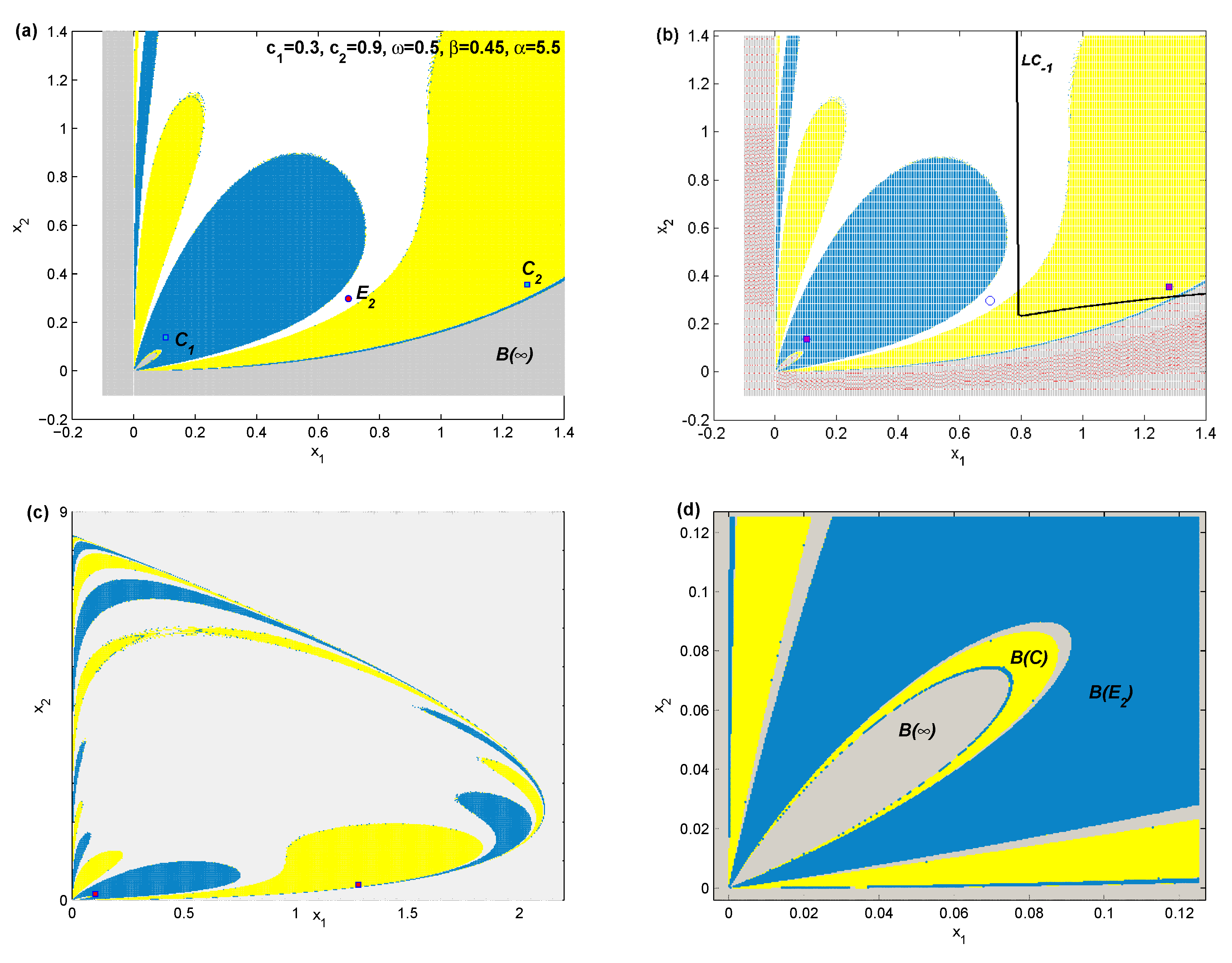
5. Non-Invertibility and Critical Curves

Suppose that the time evolution for the behavior of the two firms is formed by an iteration of the map $T:(x_1,x_2)\to ({\acute{x}}_1,{\acute{x}}_2)$ defined by,

$$T:\left\{\begin{array}{c}{\acute{x}}_1=x_1+\alpha x_1\left(\frac{x_2}{{\left(x_1+x_2\right)}^2}-c_1\right),\hfill \\ {\acute{x}}_2=x_2+\beta \left(\frac{\omega }{c_2}-x_1-x_2+(1-\omega )\sqrt{\frac{x_1}{c_2}}\right).\hfill \end{array}\right.$$

(16)

where we set $x_{1,t+1}={\acute{x}}_1$ and $x_{2,t+1}={\acute{x}}_2$ in (10). The map defined in (16) is a noninvertible map as for a given point $({\acute{x}}_1,{\acute{x}}_2)\in {\mathbb{R}}^2$ the number of solutions of the algebraic system (16) on the variables $x_1$ and $x_2$ may be zero, 2, or 4. According to those solutions, we can subdivide the phase plane into zones, $Z_i$ and the index i denotes the number of rank-1 preimages. These preimage points characterize points in the corresponding zone in the phase plane. As we can see from Figure 5 that the phase plane is quite complicated. In order to identify those zones, we should calculate the preimage points in the phase plane.

It is reported in [26,27] that any two contiguous zones are different in the number of real preimages by two. It is also reported that there may be two or more identical preimages on the critical curve indicated by $LC$. As our map is a noninvertible map and does not permit us to calculate inverse points of the phase plane, we instead calculate the set $L{C}_{-1}$ containing all the points at which the determinant of Jacobian of (16) vanishes,

$$L{C}_{-1}=\left\{\left(x_1,x_2\right)\in {\mathbb{R}}^2:detJ(x_1,x_2)=0\right\},$$

(17)

and then $LC=T\left(L{C}_{-1}\right)$. For the same set of parameters’ values used in Figure 5a, we only depict in Figure 5b the numerical computation of $L{C}_{-1}$ as it is hard to plot $LC$.

Proposition 1.

The number of real preimages of the point $({\acute{x}}_1,{\acute{x}}_2)=\left(0,{\mathring{x}}_2\right)\in {\mathbb{R}}_{+}^2$ are:

• only one that is$\left(0,\frac{c_2{\mathring{x}}_2-\omega \beta }{c_2(1-\beta )}\right)$,
• 2 or 4 under the condition$\alpha c_1\ge 1$.

Proof. 

Substituting $({\acute{x}}_1,{\acute{x}}_2)=\left(0,{\mathring{x}}_2\right)$ in (16) we get,

$$\begin{array}{c}0=x_1\left(1-\alpha c_1+\frac{\alpha x_2}{{\left(x_1+x_2\right)}^2}\right),\hfill \\ {\mathring{x}}_2=x_2+\beta \left(\frac{\omega }{c_2}-x_1-x_2+(1-\omega )\sqrt{\frac{x_1}{c_2}}\right).\hfill \end{array}$$

(18)

The first equation in (18) represents a product equalling zero if at least one of its factors becomes zero. So we consider the following two cases:

• Case 1: $x_1=0$. Substituting this case in the second equation of (18) and solving algebraically with respect to $x_2$ we get only one preimage point that is $\left(0,\frac{c_2{\mathring{x}}_2-\omega \beta }{c_2(1-\beta )}\right)$.
• Case 2: $1-\alpha c_1+\frac{\alpha x_2}{{\left(x_1+x_2\right)}^2}=0$. This condition can be rewritten as

  $${\left(x_1+x_2\right)}^2=\frac{\alpha x_2}{\alpha c_1-1},$$

  (19)

  which must be positive under the condition, $\alpha c_1\ge 1$. Substituting (19) in the second equation of (18) and solving algebraically with respect to $x_2$ we get

  $${\mathring{x}}_2=x_2+\frac{\beta \omega }{c_2}-\beta \sqrt{\frac{\alpha x_2}{\alpha c_1-1}}+\frac{\beta (1-\omega )}{\sqrt{c_2}}\sqrt{\sqrt{\frac{\alpha x_2}{\alpha c_1-1}}-x_2}.$$

  (20)
  Equation (20) is a nonlinear algebraic equation that can not be explicitly solved with respect to $x_2$. Instead we can solve it numerically at the parameter’s values, $c_1=0.3,c_2=0.9,\omega =0.5,\beta =0.45$ and $\alpha =5.5$. It is clear that at those values the condition $\alpha c_1\ge 1$ is satisfied. Furthermore, the numerical calculations show that if $0.102<{\mathring{x}}_2<0.282$ we get four real preimages while $0\le {\mathring{x}}_2\le 0.102$ or ${\mathring{x}}_2\ge 0.282$ we get only two real preimages. For example, assume ${\mathring{x}}_2=0.282$ the two preimages are $\left(6.156847367,1.034232630\right)$ and $\left(8.563457131,2.407033129\right)$. □

It is worth mentioning here that the map (16) belongs to the family of maps defined in ([28,29,30]). Those maps are defined in the form $({\acute{x}}_1,{\acute{x}}_2)=\left(\frac{N(x_1,x_2)}{D(x_1,x_2)},G(x_1,x_2)\right)$. This family of maps is defined in every point in the phase plane except the points $(x_1,x_2)\in {\mathbb{R}}^2$ such that the denominator vanishes ($D(x_1,x_2)=0$) and their preimages of any rank. Our map takes the form $0/0$ because $N(x_1,x_2)=0$ and $D(x_1,x_2)=0$ at only one point which is the origin $Q=\left(0,0\right)$. This point is called a focal point [28]. As in [23], all the points satisfying the condition $D(x_1,x_2)=0$ form a set of non-definition points and is denoted by ${\xi }_S$ and in our paper it is represented by the line, ${\xi }_S=\left\{(x_1,x_2)\in {\mathbb{R}}^2:x_2=-x_1\right\}$ and its prefocal set is defined by ${\xi }_Q:x_2=0$. For more properties of this focal point and the emergence of lobes in the suggested map, the readers are advised to see [23].

6. Conclusions

In the current work, we have introduced a Cournot duopoly game between two competed firms adopting different mechanisms for updating their outputs. As in [18,23] the first firm has chosen to behave rationally based on a gradient-based mechanism while the second firm has entered the competition with certain profit. Our current model is more general than the one studied in [18] and differs from the other discussed in [23], however, they are similar in the mechanism adopted by the first competed firm. Our discussion has shown that the game’s equilibrium can lose its stability via two different routes of chaotic dynamics. Those routes are formed due to the coexistence of period-doubling and Neimark–Sacker bifurcation. Since our game’s map includes many parameters, this has given rise to a variety of dynamic behavior of the map such as converging to the equilibrium points, periodic cycles, chaotic dynamics and closed invariant curves. We have also investigated some global properties that have given more insights into the evolution of the game. Furthermore, the noninvertibility of the map has been discussed and the appearance of lobes due to the focal point has been reported.

Our motivation in this paper is that the adoption of different mechanisms than those used in [18,23] which has made our game’s map more complicated. In addition, our model has generalized the other model discussed in [18] beside the rich analysis given for the global analysis. Our future works are to apply the suggested mechanism in this paper in a sequential quantity competition, such as one given by Stackelberg games.