Multiple Periodic Solutions and Fractal Attractors of Differential Equations with n-Valued Impulses

Abstract

Ordinary differential equations with n-valued impulses are examined via the associated Poincaré translation operators from three perspectives: (i) the lower estimate of the number of periodic solutions on the compact subsets of Euclidean spaces and, in particular, on tori; (ii) weakly locally stable (i.e., non-ejective in the sense of Browder) invariant sets; (iii) fractal attractors determined implicitly by the generating vector fields, jointly with Devaney’s chaos on these attractors of the related shift dynamical systems. For (i), the multiplicity criteria can be effectively expressed in terms of the Nielsen numbers of the impulsive maps. For (ii) and (iii), the invariant sets and attractors can be obtained as the fixed points of topologically conjugated operators to induced impulsive maps in the hyperspaces of the compact subsets of the original basic spaces, endowed with the Hausdorff metric. Five illustrative examples of the main theorems are supplied about multiple periodic solutions (Examples 1–3) and fractal attractors (Examples 4 and 5).

1. Introduction

The theory of impulsive differential equations and inclusions has been systematically developed (see e.g., the monographs [1,2,3,4], and the references therein), among other things, especially because of many practical applications (see e.g., References [1,4,5,6,7,8,9,10,11]). These applications concern fluctuations of pendulum systems under impulsive effects, remittent oscillators, population dynamics, oxygen-driven self-cycling fermentation process, nutrient-driven self-cycling fermentation process, various impulsive drug effects, optimal impulsive vaccination for an SIR control model, an SEIRS epidemic model, malaria vector model, impulsive insecticide spraying, HIV induction-maintenance therapy, and so forth.

The impulsive maps can be deterministic or stochastic (random), crisp or fuzzy, state dependent or independent, time dependent or independent, single-valued or multivalued. Here, we will be exclusively interested in multivalued, deterministic non-fuzzy state and time independent impulses in subsets of Euclidean spaces. A particular attention will be paid to a subclass of n-valued maps (see Definition 1 below), whence the title of our article. For other sorts of multivalued impulses, see e.g., (Chapter 11 in Reference [12]), References [13,14,15,16,17,18].

As far as we know, the differential equations with n-valued impulses have been tendentiously considered only in Reference [19] for multiple periodic solutions. On the other hand, the recent research of n-valued maps is very active in the topological (i.e., mainly Nielsen) fixed point theory (see e.g., References [20,21] and the earlier survey article of Brown in the handbook [22]). This research is far from being trivial, because there is for instance nothing known about the lower estimates for the number of periodic points of such maps, especially because the number of points of their iterates can be quite arbitrary in general. Moreover, it seems to be difficult to find conditions under which the iterates have an exact given number of points.

Relaxing the strict requirement of exactly n-values in Definition 1 below, we can consider the union operators of n single-valued maps, called the Hutchinson-Barnsley operators. These operators play a crucial role in constructing the fractals as attractors of iterated function systems (see References [23,24]). This relaxation makes the study in a certain sense more liberal, but the n-valued Hutchinson-Barnsley operators then become nothing else but split n-valued maps, which might not be so interesting. Nevertheless, the application of the deep results for the iterated function systems, including the chaotic dynamics on the Hutchinson-Barnsley (fractal) attractors, to impulsive differential equations via the Poincaré translation operators along the trajectories is quite original.

Besides these two novelty applications, our research in this field can be justified by a simple argument that the n-valued impulses extend with no doubts the variability in practical applications. For instance, the repeated vaccination need not be always the same, but they can differ each from other just by finitely many possibilities (e.g., when the doctors have at the same time to their disposal vaccines made by n different producers).

Our paper is organized as follows. After the useful definitions in Preliminaries, we will recall the basic properties and results about n-valued maps (in Section 3) and the Hutchinson-Barnsley operators (in Section 4). These results are neither new, but (in case of n-valued maps) nor so well known. New and original are the applications of these results to impulsive differential equations in ${\mathbb{R}}^n$ (in Section 5) and ${\mathbb{R}}^n/{\mathbb{Z}}^n$ (in Section 6), jointly with the obtained theorems about topological fractals and deterministic chaos in the sense of Devaney (in Section 7). Several illustrative examples are supplied in Section 5 and Section 6, jointly with concluding remarks in Section 8.

2. Preliminaries

In the entire text all topological spaces will be metric. A space X is an absolute neighbourhood retract (written $X\in \mathrm{ANR}$) if, for every space Y and every closed subset $A\subset Y$, each continuous map $f:A\to X$ is extendable over some open neighbourhood U of A in Y. A space X is an absolute retract (written $X\in \mathrm{AR}$) if each $f:A\to X$ is extendable over Y. Evidently, if $X\in \mathrm{AR}$, then $X\in \mathrm{ANR}$.

By a polyhedron, we understand as usually a triangulable space. It is well known that every polyhedron is an ANR-space. An important example of a compact polyhedron will be for us a torus. By the n-torus${\mathbb{T}}^n$, $n\ge 1$, we will mean here either the factor space ${\mathbb{R}}^n/{\mathbb{Z}}^n={(\mathbb{R}/\mathbb{Z})}^n$ or the Cartesian product $\underset{n-\mathrm{times}}{\underbrace{S^1\times \dots \times S^1}}$, where $\mathbb{R}$ denotes the set of reals, $\mathbb{Z}$ denotes the set of integers, and

$$S^1:=\{x\in {\mathbb{R}}^2\mid \left|x\right|=1\}=\{z={\mathrm{e}}^{2\pi s\mathrm{i}}\mid s\in [0,1]\}.$$

In particular, for $n=1$, ${\mathbb{T}}^1=S^1$ becomes a circle.

If not explicitly specified, we will not distinguish between the additive and multiplicative notations, because the logarithm map ${\mathrm{e}}^{2\pi s\mathrm{i}}\to s$, $s\in [0,1]$, establishes an isomorphism between these two representations.

Let us also note that the relation between the Euclidean space ${\mathbb{R}}^n$ and its factorization ${\mathbb{R}}^n/{\mathbb{Z}}^n$ can be realized by means of the natural projection, sometimes also called a canonical mapping, $\tau :{\mathbb{R}}^n\to {\mathbb{R}}^n/{\mathbb{Z}}^n$, $x\to \left[x\right]$, where the symbol $\left[x\right]:=\{y\in {\mathbb{R}}^n\mid (y-x)\in {\mathbb{Z}}^n\}$ stands for the equivalent class of elements with x in ${\mathbb{R}}^n/{\mathbb{Z}}^n$, that is, ${\mathbb{R}}^n/{\mathbb{Z}}^n:=\{\left[x\right]\mid x\in {\mathbb{R}}^n\}$, where $\left[x\right]=x+{\mathbb{Z}}^n$, $x\in {[0,1)}^n$.

By a multivalued map $\phi :X⊸Y$, we understand $\phi :X\to 2^Y\backslash \{\varnothing \}$. In the entire text, we will still assume that $\phi$ has closed values.

A multivalued map $\phi :X⊸Y$ is said to be continuous if, for every open $U\subset Y$, the set $\{x\in X\mid \phi (x)\subset U\}$ is open in X and at the same time if, for every closed $V\subset Y$, the set $\{x\in X\mid \phi (x)\subset V\}$ is closed in X.

Obviously, in the single-valued case, if $f:X\to Y$ is continuous in a multivalued sense, then it is continuous in the usual (single-valued) sense. Furthermore, every continuous map $\phi :X⊸Y$ has a closed graph ${\Gamma }_{\phi }:=\left\{(x,y)\in X\times Y\mid y\in \phi \left(x\right)\right\}$, but not vice versa. If $\phi :X⊸Y$ is continuous with compact values and $A\subset X$ is compact, then $\phi \left(A\right)$ is compact, too. The composition $\psi \circ \phi :X⊸Z$ of two continuous maps with compact values, $\phi :X⊸Y$ and $\psi :Y⊸Z$, is again continuous with compact values. For more details, see for example, References [25,26].

For the single-valued compact continuous maps $f:X\to X$, where $X\in \mathrm{ANR}$, we can define the global topological invariants, namely the Lefschetz number$L\left(f\right)\in \mathbb{Z}$ and the Nielsen number $N\left(f\right)\in \mathbb{N}\cup \left\{0\right\}$. If, in particular, $X\in \mathrm{AR}$, then $L\left(f\right)=1$ and $N\left(f\right)=1$.

For the single-valued continuous maps on tori, $f:{\mathbb{T}}^n\to {\mathbb{T}}^n$, the Anosov-type equality $N\left(f\right)=\left|L\left(f\right)\right|$ holds. For the single-valued continuous maps on the circle ($n=1$), $f:S^1\to S^1$, we can also define their degree $deg\left(f\right):=1-L\left(f\right)$. If $S^1=\mathbb{R}/\mathbb{Z}$, then $deg\left(f\right)=\tilde{f}\left(1\right)-\tilde{f}\left(0\right)$, where $\tilde{f}:\mathbb{R}\to \mathbb{R}$ denotes the lift of f.

Besides their existence property, when the existence of a fixed point $x=f\left(x\right)$ of a compact continuous $f:X\to X$, $X\in \mathrm{ANR}$, is implied by $L\left(f\right)\ne 0$, resp. by $N\left(f\right)>0$, or in particular for $X=S^1$ by $deg\left(f\right)\ne 1$ (i.e., $\tilde{f}\left(1\right)-\tilde{f}\left(0\right)\ne 1$), all these numbers are invariant under a compact continuous homotopy, namely $L\left(f_0\right)=L\left(f_1\right)=L\left(f_{\mu }\right)$, $N\left(f_0\right)=N\left(f_1\right)=N\left(f_{\mu }\right)$, and (for $X=S^1$) $deg\left(f_0\right)=deg\left(f_1\right)=deg\left(f_{\mu }\right)=f_0\left(1\right)-f_0\left(0\right)=f_1\left(1\right)-f_1\left(0\right)=f_{\mu }\left(1\right)-f_{\mu }\left(0\right)$, for all $\mu \in [0,1]$.

The Nielsen number $N\left(f\right)$ of a continuous map $f:X\to X$, where $X\in \mathrm{ANR}$, gives still the lower estimate of the number of fixed points, that is, $N\left(f\right)\le \#\left\{x\in X\mid x=f\left(x\right)\right\}$, where the symbol # stands for the cardinality of the fixed point set $\left\{x\in X\mid x=f\left(x\right)\right\}$.

For the definitions and more details, see e.g., References [27,28].

Since in Section 4 and Section 7 we will also consider hyperspaces endowed with the Hausdorff metric $d_H$, it will be convenient to recall finally their definitions. Hence, if $(X,d)$ is a metric space endowed with the metric d, then the induced hyperspace $(K\left(X\right),d_H)$ is defined as

$$K\left(X\right):=\left\{Y\subset X\mid Y\mathrm{is}\mathrm{a}\mathrm{compact}\mathrm{subset}\mathrm{of}X\right\},$$

and the Hausdorff metric $d_H(·,·):=K\left(X\right)\times K\left(X\right)\to [0,\infty )$ is induced by d as follows:

$$d_H(A,B):=max\left\{\underset{a\in A}{sup}d(a,B),\underset{b\in B}{sup}d(A,b)\right\}=max\left\{\underset{a\in A}{sup}\left(\underset{b\in B}{inf}d(a,b)\right),\underset{b\in B}{sup}\left(\underset{a\in A}{inf}d(a,b)\right)\right\},$$

where $d(a,B)$ and $d(A,b)$ stand for the distances between points $a,b$ and sets $A,B$, respectively. For more details, see for example, References [24,25,29,30].

3. $\mathit{N}$-Valued Maps

The topological fixed point theory for multivalued maps has been developed in two main directions: (i) for admissible maps (in the sense of Górniewicz) and their particular cases like acyclic maps, $R_{\delta }$-maps, and so forth (see e.g., References [22,25,26], and the references therein), and (ii) for n-valued maps (see e.g., References [20,21,22,31,32,33,34,35,36,37,38,39,40,41,42,43,44,45,46,47,48]) and their generalizations like n-acyclic maps (see e.g., Reference [49]) and weighted maps (see e.g., Reference [50]). In the present paper, we will be exclusively interested in the second class of n-valued maps whose research made a big progress in the recent years.

Let us recall their definition and some basic properties.

Definition 1.

Ann-valued map $\phi :X⊸Y$is a continuous multivalued mapping that associates to each$x\in X$an unordered subset of exactly n points of Y. We say that an n-valued map φ is split if there are single-valued continuous maps $f_1,\dots ,f_n:X\to Y$ such that $\phi \left(x\right)=\left\{f_1\left(x\right),\dots ,f_n\left(x\right)\right\}$, for all $x\in X$.

One can readily check that unlike to admissible maps, where the sets of values are compact and connected (i.e., continua), those of n-valued maps are disconnected. Moreover, unlike to the above definition of general multivalued maps, for the continuity of n-valued maps is sufficient if, for every closed $V\subset Y$, the set $\left\{x\in X\mid \phi \left(x\right)\subset V\right\}$ is closed in X.

Lemma 1

(splitting lemma; cf. References [44,47,51]). If X is simply connected and locally path-connected, then every n-valued map $\phi :X⊸Y$ is split.

Let us recall that X is simply connected if and only if it is path-connected and its fundamental (first homotopy) group is trivial.

Lemma 2

(cf. Reference [33], Theorem 2.1). Any n-valued map ${\phi }_1:X⊸Y$ which is homotopic in an n-valued way (i.e., via a continuous mapping ${\phi }_t:X\times [0,1]⊸Y$ such that ${\phi }_t\left(x\right)$ has exactly n-points, for all $(x,t)\in X\times [0,1])$ to a split n-valued map ${\phi }_0:X⊸Y$ (written ${\phi }_t\sim {\phi }_0$) is also split.

If X is a compact $\mathrm{ANR}$- space and $f:X\to X$ is a single-valued continuous self-map, then the Nielsen number $N\left(f\right)$ of f is well defined (see e.g., References [27,28]). Since a (compact) $\mathrm{ANR}$-space is (uniformly) locally contractible, and so locally path-connected, if X is still simply connected, then all fixed points of f belong to a single (same) fixed point class, whose index is $L\left(f\right)$, where $L\left(f\right)$ stands for the Lefschetz number of f. For its definition and more details, see for example, Reference [27]. Therefore, if X is still simply connected, then $N\left(f\right)=1$ if $L\left(f\right)\ne 0$, and $N\left(f\right)=0$ if $L\left(f\right)=0$.

Summing up, if X is a simply connected compact $\mathrm{ANR}$-space, then the Nielsen relation of any self-map $g_k:X\to X$ homotopic to $f_k:X\to X$ (written $g_k\sim f_k$) is trivial, that is, $N\left(g_k\right)=N\left(f_k\right)\le 1$, for $k=1,\dots ,n$. Subsequently, the Nielsen numbers $N\left(\psi \right)$ and $N\left(\phi \right)$ of homotopic n-valued maps $\psi =\left\{g_1,\dots ,g_n\right\}:X⊸X$ and $\phi =\left\{f_1,\dots ,f_n\right\}:X⊸X$ can be simply defined and calculated by the formula:

$$N\left(\psi \right)=N\left(\phi \right):=\sum _{k=1}^{n}N\left(f_k\right)=\#\left\{k=1,\dots ,n\mid L\left(f_k\right)\ne 0\right\},$$

(1)

where the symbol # denotes the cardinality of a given set.

If, in particular, X is a compact $\mathrm{AR}$-space, then formula (1) takes the form

$$N\left(\psi \right)=N\left(\phi \right):=\sum _{k=1}^{n}N\left(f_k\right)=n,$$

(2)

because $L\left(f_k\right)=1$, for all $k=1,\dots ,n$.

Remark 1.

Let us note that (compact) simply connected $\mathit{ANR}$-spaces are not necessarily (compact) $\mathit{AR}$-spaces. For example, every n-dimensional unit sphere $S^n$, where $n\ge 2$, is a simply connected $\mathit{ANR}$-space, but not contractible, and so an $\mathit{AR}$-space. Moreover, $L\left({\mathrm{id}}_{S^2}\right)=2$ but, according to (1), $N\left({\mathrm{id}}_{S^2}\right)=1$.

Remark 2.

According to the example due to Jezierski [43], there exists a continuous map $\phi :{\mathcal{K}}^2⊸{\mathcal{K}}^2$, where ${\mathcal{K}}^2\subset \mathbb{C}$ is a two-dimensional closed ball in the complex plane $\mathbb{C}$, whose values consist of 1 or 2 or 3 points, which is fixed point free.It justifies the assumption of exactly n-valued maps in Definition 1.

Of course, the assumption of a simple connectedness of X is not necessary for the splitting of n-valued self maps $\phi :X⊸X$. For instance, if $X=S^1=\mathbb{R}/\mathbb{Z}$, then an n-valued map $\phi :S^1⊸S^1$ of degree $\mathrm{Deg}\left(\phi \right)$ (for its definition, see for example, Theorem 2.1 in Reference [33]) is split if and only if $\mathrm{Deg}\left(\phi \right)$ is a multiple of n (see Corollary 5.1 in Reference [33]).

In the case of splitting, we have to our disposal the following lemma.

Lemma 3

(cf. Theorems 2.2 and 2.3 in Reference [33]). If $\phi :S^1⊸S^1$ is a split n-valued map, then its degree $\mathrm{Deg}\left(\phi \right)$ equals n-times the classical degree of the maps in the splitting. Furthermore, if $\psi :S^1\to S^1$ is homotopic in an n-valued way to φ ($\psi \sim \phi$), then

$$\mathrm{Deg}\left(\psi \right)=\mathrm{Deg}\left(\phi \right)=ndeg\left(f_1\right)=\dots =ndeg\left(f_n\right)=n\left[{\tilde{f}}_1\left(1\right)-{\tilde{f}}_1\left(0\right)\right],$$

(3)

where ${\tilde{f}}_1:\mathbb{R}\to \mathbb{R}$ is the lift of $f_1:\mathbb{R}/\mathbb{Z}\to \mathbb{R}/\mathbb{Z}$.

In the non-split case, the situation becomes obviously more delicate. Nevertheless, for $X=S^1=\mathbb{R}/\mathbb{Z}$, we have even the Wecken property.

Lemma 4

(cf. Theorem 5.1 in Reference [33]). If $\phi :S^1⊸S^1$ is an n-valued map of degree $\mathrm{Deg}\left(\phi \right)$, then $N\left(\phi \right):=\left|n-\mathrm{Deg}\left(\phi \right)\right|$ holds for the Nielsen number $N\left(\phi \right)$ of φ, and there is an n-valued map, say ψ, homotopic to φ (i.e., $\psi \sim \phi$), that has exactly $\left|n-\mathrm{Deg}\left(\phi \right)\right|=\left|n-\mathrm{Deg}\left(\psi \right)\right|$ fixed points (i.e., the Wecken property).

Remark 3.

Observe that the equalities (3) in Lemma 3 can be expressed in terms of the Nielsen numbers as follows:

$$N\left(\psi \right)=N\left(\phi \right)=\left|n-\mathrm{Deg}\left(\phi \right)\right|=n|1-deg\left(f_1\right)|=n|1-\left[{\tilde{f}}_1\left(1\right)-{\tilde{f}}_1\left(0\right)\right]|,$$

(4)

because $N\left(f_1\right)=|L\left(f_1\right)|=|1-deg\left(f_1\right)|=|1-\left[{\tilde{f}}_1\left(1\right)-{\tilde{f}}_1\left(0\right)\right]|$.

Now, we will briefly sketch the definition and basic properties of the Nielsen number for n-valued maps on compact polyhedra, which is essentially due to Schirmer [46] (see also the recent Reference [20]). The restriction to compact polyhedra is caused by the application of such a fixed point index in Reference [46]. For more general indices, see for example, References [40,48,49]. On the other hand, it will be quite sufficient for our needs in applications.

Using the fact that n-valued maps are locally (but not globally) equivalent to n single-valued continuous functions, which is important for the choice of a suitable index of isolated fixed points, Schirmer proceeded in Reference [46] analogously to a single-valued case ($n=1$). Of course, all the technicalities (especially those related to the fixed point index) must have been appropriately elaborated there. For an alternative approach via the lifting classes, see Reference [20].

Hence, let X be a compact polyhedron and $\phi :X⊸X$ be an n-valued self-map. To obtain the Nielsen number $N\left(\phi \right)$ of $\phi$, the fixed points of $\phi$ were at first divided into finitely many equivalent classes (see Theorem 5.2 in Reference [46]), called fixed point classes or Nielsen classes. Then a suitable fixed point index was associated with each fixed point class. The (Nielsen) classes with non-zero index are called essential. The Nielsen number $N\left(\phi \right)$ of $\phi$ is the number of essential (Nielsen) fixed point classes.

The Nielsen number $N\left(\phi \right)$ gives the lower estimate of the number of fixed points of $\phi$, that is, that any n-valued self-map $\phi :X⊸X$ has at least $N\left(\phi \right)$ fixed points (cf. Theorem 5.4 in Reference [46]). Furthermore, $\phi$ satisfies the homotopy invariance, that is, if ${\phi }_t:X\times [0,1]⊸X$ is an n-valued homotopy, then $N\left({\phi }_0\right)=N\left({\phi }_1\right)$ (cf. Theorem 6.5 in Reference [46]).

Remark 4.

Although the Anosov property, namely that $N\left(\phi \right)=\left|L\left(\phi \right)\right|$, holds for n-valued maps on $S^1$, because $\mathrm{Deg}\left(\phi \right)=n-L\left(\phi \right)$, it is no longer true for higher dimensional tori ${\mathbb{T}}^n$, where $n>1$, which complicates the calculations. Nevertheless, if $\phi =\left\{f_1,\dots ,f_n\right\}:X⊸X$ is a split n-valued self-map on a compact polyhedron X, then $N\left(\phi \right)={\sum }_{k=1}^{n}N\left(f_k\right)$ (cf. Corollary 7.2 in Reference [46]). If, in particular, φ is an n-valued constant, then $N\left(\phi \right)=n$ (cf. Corollary 7.3 in Reference [46]).

Remark 5.

Observe that, unlike to equalities (1) and (2), compact polyhedra in Remark 4 need not be simply connected. Let us note that every compact $\mathit{ANR}$-space is homotopically equivalent to some polyhedron (see e.g., Reference [26]). On the other hand, since any two continuous maps $f,g:X\to X$, where X is a compact absolute retract, are homotopic and $L\left(f\right)=1$ (see again e.g., Reference [26]), we get that $N\left(f\right)=N\left(g\right)=1$, and subsequently we can put $N\left(\phi \right)={\sum }_{k=1}^{n}N\left(f_k\right)=n$, as in (2).

4. Hutchinson-Barnsley’s Operators

As far as we know, there are no nontrivial results about the periodic point theory, or more precisely periodic orbit theory, for n-valued maps with $n>1$. The reason consists in an almost uncontrollable enormous variability of their iterates, by which the existence (and even worse multiplicity) problems of nontrivial periodic orbits seem to be a difficult task.

On the other hand, the theory of iterated function systems (IFS), originated by Hutchinson [23] and extended and popularized by Barnsley [24], allows us to construct compact invariant subsets $A\subset X$ of a complete metric space $(X,d)$ of the Hutchinson-Barnsley operators

$$\phi :=\bigcup _{k=1}^n{f}_k:X⊸X,\mathrm{i}.\mathrm{e}.,A=\phi \left(A\right)=\bigcup _{k=1}^n\bigcup _{x\in A}{f}_k\left(x\right),$$

provided $f_k:X\to X$, $k=1,\dots ,n$, are contractions, that is,

$$\exists L_k\in [0,1):d(f_k\left(x\right),f_k\left(y\right))\le L_{k}d(x,y)\forall x,y\in X,k=1,\dots ,n.$$

Since a unique A can be obtained as the limit ${lim}_{m\to \infty }{\phi }^m\left(A_0\right)=A$, that is, $lim{d}_H(A_m,A)=0$, where $A_0\subset X$ is an arbitrary compact subset, $A_m=\phi \left(A_{m-1}\right)$, $m=1,2,\dots$, and $d_H$ stands for the Hausdorff metric (see Section 2), A is called the (global) attractor of the iterated function system (IFS) $\left\{X;f_1,\dots ,f_n\right\}$. Moreover, the inequality

$$d_H(A_m,A)\le \frac{L^m}{1-L}{d}_H(A_0,\phi \left(A_0\right)),$$

(5)

where $L={max}_{k=1,\dots ,n}{L}_k$, holds for the m-th iterate ${\phi }^m\left(A_0\right)=A_m$ of $\phi$, for all $m=1,2,\dots$

The attractor A has usually a fractal structure, whose fractal dimension $dimA$ can be estimated from above (i.e., to get its upper bound $dimA\le D$) by means of the Moran-Hutchinson formula (cf. References [23,24])

$$\sum _{k=1}^n{L}_k^D=1\left(\mathrm{for}L=L_1=\dots =L_n:D=\frac{logn}{log\frac{1}{L}}\right),$$

(6)

provided the sets $f_k\left(A\right)$, $k=1,\dots ,n$, are either totally disconnected, that is,

$$f_j\left(A\right)\cap f_k\left(A\right)=\varnothing ,\mathrm{for}\mathrm{all}j,k=1,\dots ,n;j\ne k,$$

(7)

or just touching (i.e., neither (7), nor with overlaps).

If, in particular, $f_k$ are similitudes, that is,

$$d(f_k\left(x\right),f_k\left(y\right))=L_{k}d(x,y),\mathrm{for}\mathrm{all}x,y\in X,k=1,\dots ,n,$$

then we get $dimA=D$.

Observe that condition (7) is much stronger than the one required in Definition 1 for n-valued maps, because $\phi {|}_A:A⊸A$ is certainly continuous and every image set $\phi {|}_A\left(x\right)$ must contain exactly n-points, for each $x\in A$. In other words, $\phi {|}_A$ is in particular a split n-valued map on a compact invariant set $A\subset X$.

Moreover, one can prove that every $f_k{|}_A$, $k=1,\dots ,n$, must be injective, because otherwise if there are two points, say $a_1,a_2\in A$, such that $f_k\left(a_1\right)=f_k\left(a_2\right)=a\in A$, then $a\in A$ would have two addresses, which is impossible (see e.g., Reference [24]). Therefore, we can assume without any loss of generality that $f_k{|}_A$ are under (7) invertible, for all $k=1,\dots ,n$. Furthermore, every inversion $f_k^{-1}:f_k\left(A\right)\to A$ is a continuous map, for every $k=1,\dots ,n$.

Hence, we can define the discrete dynamical system $(A,S)$ by the mapping $S:A\to A$, where

$$S\left(a\right):=\bigcup _{k=1}^n{f}_k^{-1}\left(a\right),$$

(8)

which can be uniquely defined by $S\left(a\right):=f_k^{-1}\left(a\right)$, provided $a\in f_k\left(A\right)$. The system $(A,S)$ is called the shift dynamical system, associated with the iterated function system $\left\{A;f_1,\dots ,f_n\right\}$. It can be proved that it is chaotic in the sense of Devaney (see e.g., References [24,30]), that is,

(i)

S is sensitive to initial conditions,

(ii)

S is transitive (if $U,V\subset A$ are open subsets, then there exists an integer $n^{*}$ such that $U\cap S^{n^{*}}\left(V\right)\ne \varnothing$),

(iii)

the set of periodic points of S is dense in A.

We can extend the definition of S to the hyperspace $K\left(A\right):=\left\{B\subset A\mid B\mathrm{is}\mathrm{a}\mathrm{compact}\mathrm{subset}\mathrm{of}A\right\}$, endowed with the Hausdorff metric $d_H$. Hence, let us define the hypermap $S^{*}:K\left(A\right)\to K\left(A\right)$, where

$$S^{*}\left(B\right):=\bigcup _{k=1}^n{f}_k^{-1}\left(B\right),B=\bigcup _{x\in B}\in K\left(A\right).$$

(9)

It is well known (see e.g., References [23,24]) that $(K\left(A\right),d_H)$ is also compact and $S^{*}$ is continuous in the metric $d_H$.

Haase Theorem 1 in Reference [52] has proved that the system $(K\left(A\right),S^{*})$ is also chaotic in the sense of Devaney with respect to the Hausdorff metric $d_H$, provided (5) holds.

Summing up, we can formulate the following two well known propositions.

Proposition 1

(cf. References [23,24]). The iterated function system $\left\{X;f_1,\dots ,f_n\right\}$, where $(X,d)$ is a complete metric space and $f_k:X\to X$ are contractions, for all $k=1,\dots ,n$, admits a unique global attractor $A\in K\left(X\right)$, which can be obtained as the limit ${lim}_{m\to \infty }{\phi }^m\left(A_0\right)=A$, that is, ${lim}_{m\to \infty }{d}_H(A_m,A)=0$, where $A_0\subset X$ is an arbitrary compact subset and $A=\phi \left(A\right)$, $A_m={\phi }^m\left(A_0\right)$, $\phi :={\cup }_{k=1}^n{f}_k:X⊸X$.

Moreover, the inequality (5) holds for the successive approximations $A_m$, $m=1,2,\dots$, of the attractor A, whose fractal dimension $dimA$ can be estimated from above (i.e., $dimA\le D$) by means of the Moran-Hutchinson formula (6).

Proposition 2

(cf. References [24,52]). Let $\left\{X;f_1,\dots ,f_n\right\}$ be an iterated function system as in Proposition 1. Assume, furthermore, that the sets $f_k\left(A\right)$ are totally disconnected, for all $k=1,\dots ,n$ (see (7)). Then the shift dynamical system $(A,S)$, where $S:A\to A$ is defined in (8), which is associated with the iterated function system $\left\{A;f_1,\dots ,f_n\right\}$, is chaotic in the sense of Devaney. The same is true for the system $(K\left(A\right),S^{*})$, where the hypermap $S^{*}:K\left(A\right)\to K\left(A\right)$ is defined in (9), with respect to the Hausdorff metric $d_H$.

Remark 6.

Since every contraction $f_k$ on a complete metric space X has, for every $k=1,\dots ,n$, exactly one fixed point, the Hutchinson-Barnsley operator $\phi :={\bigcup }_{k=1}^n{f}_k:X⊸X$ must have at most n fixed points. Since the attractor $A\subset X$ is compact, and so complete, all the fixed points of the restricted contractions $f_k{|}_A:A\to A$, $k=1,\dots ,n$, as well as of $\phi {|}_A:A⊸A$ must belong to A.

The existence of a compact invariant subset of the Hutchinson-Barnsley operator can be also obtained in the frame of topological fixed point theory (unlike to “metric” Proposition 1) as follows. Let us recall here that a metric space X is locally continuum-connected if, for each neighbourhood U of each point $x\in X$, there is a neighbourhood $V\subset U$ of x such that each point of V can be connected with x by a subcontinuum (i.e., a compact, connected subset) of U.

Proposition 3

(cf. References [29,53,54]). Let X be a connected, locally continuum-connected metric space and $f_k:X\to X$ be compact continuous maps, for all $k=1,2,\dots ,n$. Then the Hutchinson-Barnsley operator

$$\phi :=\bigcup _{k=1}^n{f}_k:X⊸X$$

possesses at least one compact invariant set, say $X_0\in K\left(X\right)$, such that $X_0=\phi \left(X_0\right)$.

If, in particular, X is a Peano continuum (i.e., compact, connected and locally connected) and $f_k:X\to X$ are continuous maps, for all $k=1,2,\dots ,n$, then φ possesses at least one compact invariant set $\phi \left(X_0\right)=X_0\subset X$ which is non-ejective in the sense of Browder, that is,

$$\begin{array}{c}\forall \epsilon >0\exists X_1\in K\left(X\right),X_1\ne X_0,and{d}_H(X_0,X_1)<\delta :\\ {\phi }^m\left(X_1\right)={\left[\bigcup _{x\in X_0}\bigcup _{k=1}^n{f}_k\left(x\right)\right]}^m\subset \left\{Y\in K\left(X\right)\mid d_H(X_0,Y)<\epsilon \right\},\forall m\ge 1.\end{array}$$

(10)

Remark 7.

The Hutchinson-Barnsley operator in Propositions 1 and 3 need not (but can) be exactly n-valued. Furthermore, the contractions $f_k$ in Proposition 1 can be more generally replaced, for the existence of a unique attractor $A\in K\left(X\right)$, by multivalued contractions with compact values. In Proposition 3, compact continuous maps $f_k$ can be also replaced, for the existence of a compact invariant set $A\in K\left(X\right)$ of φ (without uniqueness, but including (10)), by compact continuous multivalued maps with compact values. For more details and further possibilities (see References [29,53,54,55]).

Remark 8.

Let us emphasize that the maps $f_k$ as well as the Hutchinson-Barnsley operator φ can be, under the assumptions of Proposition 3, fixed point free. For instance, rotations on the circle $X=S^1$ can be so. On the other hand, the non-ejectivity (10) can be regarded as a weak local stability of an invariant set $A\in K\left(X\right)$ of φ.

5. Application to Impulsive Differential Equations in ${\mathbb{R}}^{\mathbf{n}}$

In this section, the presented results for n-valued maps will be applied to impulsive differential equations in ${\mathbb{R}}^n$.

Consider the vector differential equation

$$x^{\prime }=F(t,x),$$

(11)

where $F:\mathbb{R}\times {\mathbb{R}}^n\to {\mathbb{R}}^n$ is the Carathéodory mapping such that $F(t,x)\equiv F(t+\omega ,x)$, for some given $\omega >0$, that is,

(i)

$F(·,x):[0,\omega ]\to {\mathbb{R}}^n$ is measurable, for every $x\in {\mathbb{R}}^n$,

(ii)

$F(t,·):{\mathbb{R}}^n\to {\mathbb{R}}^n$ is continuous, for almost all (a.a.) $t\in [0,\omega ]$.

Let, furthermore (11) satisfy a uniqueness condition (e.g., a locally Lipschitz condition) and all solutions of (11) entirely exist on the whole line $(-\infty ,\infty )$.

By a (Carathéodory) solution $x(·)$ of (11), we understand a locally absolutely continuous function, that is, $x\in A{C}_{loc}(\mathbb{R},{\mathbb{R}}^n)$, which satisfies (11) for a.a. $t\in \mathbb{R}$.

We can associate to (11) the Poincaré translation operator $T_{\omega }:{\mathbb{R}}^n\to {\mathbb{R}}^n$ along its trajectories as follows:

$$T_{\omega }\left(x_0\right):=\left\{x\left(\omega \right):x(·)\mathrm{is}\mathrm{a}\mathrm{solution}\mathrm{of}\left(11\right)\mathrm{such}\mathrm{that}x\left(0\right)=x_0\right\}.$$

(12)

It is well known (see e.g., Chapter 1.1 in Reference [56]) that $T_{\omega }$ is a homeomorphism such that $T_{\omega }^k=T_{k\omega }$, (i.e., the semi-group property), for every $k\in \mathbb{N}$.

One can easily detect the one-to-one correspondence between the $k\omega$-periodic solutions of (11), that is, $x\left(t\right)\equiv x(t+k\omega )$ but $x\left(t\right)\not\equiv x(t+j\omega )$ for $j<k$, and k-periodic points of $T_{\omega }$, i.e., $x_0=T_{\omega }^k\left(x_0\right)$ but $x_0\ne T_{\omega }^j\left(x_0\right)$ for $j<k$, where $x_0=x\left(0\right)$ and $j,k$ are positive integers.

Consider also the vector impulsive differential equation

$$\left\{\begin{array}{c}{x}^{\prime }=F(t,x),t\ne t_j:=j\omega ,\mathrm{for}\mathrm{some}\mathrm{given}\omega >0,\hfill \\ x\left(t_j^{+}\right)\in I\left(x\left(t_j^{-}\right)\right),j\in \mathbb{Z},\hfill \end{array}\right.$$

(13)

where $F:\mathbb{R}\times {\mathbb{R}}^n\to {\mathbb{R}}^n$ is the Carathéodory mapping such that $F(t,x)\equiv F(t+\omega ,x)$, Equation (11) satisfies a uniqueness condition and a global existence of all its solutions on $(-\infty ,\infty )$. Let, furthermore, $I:{\mathbb{R}}^n⊸{\mathbb{R}}^n$ be a continuous impulsive mapping.

The solutions of impulsive differential Equation (13) will be also understood in the Carathéodory sense, that is, $x\in AC\left[t_j,t_{j+1}\right]$, $j\in \mathbb{Z}$. For multivalued impulses I, there need not be any longer one-to-one correspondence between the $k\omega$-periodic solutions of (13) and k-periodic orbits of the composition $I\circ T_{\omega }$. Nevertheless, every k-periodic orbit of $I\circ T_{\omega }$ implies the existence of a related $k\omega$-periodic solution of (13), and vice versa.

The first application deals with compact m-valued impulses I in (13).

Theorem 1.

Assume that $I:{\mathbb{R}}^n⊸{\mathbb{R}}^n$ is a compact m-valued map such that $I\left(K_0\right)=K_0$, where $K_0:=\overline{I\left({\mathbb{R}}^n\right)}$ is a simply connected $\mathit{ANR}$-space such that $K_0\subset K_1:=T_{\omega }\left(K_0\right)$. Then $I{|}_{K_0}$ is an m-valued split map of the form $I{|}_{K_0}=\left\{i_1,\dots ,i_m\right\}$, and subsequently the number of ω-periodic solutions of (13) is at least equal to $\#\left\{k=1,\dots ,m\mid L\left(i_k\right)\ne 0\right\}$, where L is the ordinary Lefschetz number.

Proof. 

Since I is compact and $T_{\omega }$ is a homeomorphism, $K_0:=\overline{I\left({\mathbb{R}}^n\right)}$ and $K_1:=T_{\omega }\left(K_0\right)$ must be compact sets. Since every $\mathrm{ANR}$-space is locally path-connected, $K_0$ is a compact simply connected and locally path-connected $\mathrm{ANR}$-space, and $I{|}_{K_0}:K_0⊸K_0$ is (according to Lemma 1) a split m-valued map.

Furthermore, since $T_{\mu \omega }:{\mathbb{R}}^n\to {\mathbb{R}}^n$ is also a homeomorphism, for every $\mu \in [0,1]$, the composition $I\circ T_{\mu \omega }{|}_{K_0}:K_0⊸K_0$, $\mu \in [0,1]$, is an m-valued homotopy between ($\mu =0$) $I\circ T_0{|}_{K_0}=I\circ \mathrm{id}{|}_{K_0}=I{|}_{K_0}:K_0\to K_0$, and ($\mu =1$) $I\circ T_{\omega }{|}_{K_0}:K_0⊸K_0$. According to Lemma 2, $I\circ T_{\omega }{|}_{K_0}:K_0⊸K_0$ is a split m-valued map, too.

Letting $I{|}_{K_0}=\left\{i_1,\dots ,I_m\right\}$ and applying formula (1), we get that $N(I\circ T_{\omega }{|}_{K_0})=N\left(I{|}_{K_0}\right)={\sum }_{k=1}^{m}N\left(i_k\right)=\#\left\{k=1,\dots ,m\mid L\left(i_k\right)\ne 0\right\}$. It means that the mapping $I\circ T_{\omega }{|}_{K_0}$ has at least such a number of fixed points, which determine the same number of $\omega$-periodic solutions of (13), as claimed. This completes the proof. □

Corollary 1.

Let the assumptions of Theorem 1 be satisfied. Assume additionally that $K_0$ is a (compact) $\mathit{AR}$-space. Then Equation (13) admits at least m ω-periodic solutions.

Proof. 

The claim follows immediately from Theorem 1, when replacing in the proof formula (1) by formula (2) (cf. Remark 1). □

We will supply Corollary 1 by two simple illustrative examples. The first example concerns the scalar case ($n=1$).

Example 1.

Consider the semi-linear impulsive equation

$$\left\{\begin{array}{c}{x}^{\prime }=p(t,x)x+q(t,x),t\ne t_j:=j\omega ,forsomegiven\omega >0,\hfill \\ x\left(t_j^{+}\right)\in I\left(x\left(t_j^{-}\right)\right),j\in \mathbb{Z},\hfill \end{array}\right.$$

(14)

where $p,q:{\mathbb{R}}^2\to \mathbb{R}$ are Carathéodory functions such that $p(t,x)\equiv p(t+\omega ,x)$, $q(t,x)\equiv q(t+\omega ,x)$, and the compact m-valued function $I:\mathbb{R}⊸\mathbb{R}$ satisfies $\overline{I\left(\mathbb{R}\right)}=[0,1]$, and $I\left(\right[0,1\left]\right)=[0,1]$.

The solutions $x_0(·),x_1(·)$ of $x^{\prime }=p(t,x)x+q(t,x)$ such that $x_0\left(0\right)=0$, $x_1\left(0\right)=1$ can be implicitly expressed as

$$\begin{array}{cc}\hfill x_0\left(t\right)& ={\int }_0^t{e}^{{\int }_s^{t}p(r,x_0\left(r\right))dr}q(s,x_0\left(s\right))ds,\hfill \\ \hfill x_1\left(t\right)& =e^{{\int }_0^{t}p(s,x_1\left(s\right))ds}+{\int }_0^t{e}^{{\int }_s^{t}p(r,x_1\left(r\right))dr}q(s,x_1\left(s\right))ds.\hfill \end{array}$$

Hence, the required inclusion $K_0:=[0,1]\subset K_1:=\left[T_{\omega }\left(0\right),T_{\omega }\left(1\right)\right]$ in Corollary 1 ($K_0:=[0,1]$ is obviously a compact $\mathit{AR}$-space), takes the form

$$\begin{array}{cc}\hfill 0& \ge {\int }_0^{\omega }{e}^{{\int }_s^{\omega }p(r,x_0\left(r\right))dr}q(s,x_0\left(s\right))ds,\hfill \\ \hfill 1& \le e^{{\int }_0^{\omega }p(t,x_1\left(t\right))dt}+{\int }_0^{\omega }{e}^{{\int }_s^{\omega }p(r,x_1\left(r\right))dr}q(s,x_1\left(s\right))ds.\hfill \end{array}$$

In order to satisfy the first inequality, we can assume that $q(t,x)\le 0$, for a.a. $t\in [0,\omega ]$ and all $x\in \mathbb{R}$. The second inequality can be then more restrictively rewritten into

$$e^{{\int }_0^{\omega }p(t,x_1\left(t\right))dt}\ge 1+\left|{\int }_0^{\omega }{e}^{{\int }_s^{\omega }p(r,x_1\left(r\right))dr}q(s,x_1\left(s\right))ds\right|.$$

Assuming still the existence of real constants $p_0,p_1,q_1$ such that

$$0<p_0\le p(t,x)\le p_{1}and\left|q(t,x)\right|\le q_1,for\mathrm{a}.\mathrm{a}.t\in [0,\omega ]andallx\in \mathbb{R},$$

we still require that

$$q_1\le \frac{e^{p_0\omega }-1}{\omega e^{p_1\omega }},$$

that is, jointly with $q(t,x)\le 0$,

$$-\frac{e^{p_0\omega }-1}{\omega e^{p_1\omega }}\le q(t,x)\le 0,fora.a.t\in [0,\omega ]andallx\in \mathbb{R},$$

(15)

where $0\le p_0\le p(t,x)$, for a.a. $t\in [0,\omega ]$ and all $x\in \mathbb{R}$.

Thus, the semi-linear impulsive Equation (14) admits, according to Corollary 1, at least m ω-periodic solutions, provided (15) holds jointly with $I:\mathbb{R}⊸\mathbb{R}$ being a compact m-valued function such that $\overline{I\left(\mathbb{R}\right)}=[0,1]$ and $I\left(\right[0,1\left]\right)=[0,1]$.

Now, we would like to apply Corollary 1 to the nonlinear vector impulsive differential Equation (13).

Example 2.

Consider (13), where F is as above, and assume that the inequalities

$$\left\{\begin{array}{cc}{f}_j(t,\dots ,x_j,\dots )>0\hfill & holdsforall{x}_j\ge b_j,j=1,\dots ,n,\hfill \\ f_j(t,\dots ,x_j,\dots )<0\hfill & holdsforall{x}_j\le a_j,j=1,\dots ,n,\hfill \end{array}\right.$$

(16)

hold uniformly for a.a. $t\in [0,\omega ]$ and all the remaining components of $x=(x_1,\dots ,x_n)$, where $F(t,x)={(f_1(t,x),\dots ,f_n(t,x))}^T$. Let $I:{\mathbb{R}}^n⊸{\mathbb{R}}^n$ be a compact m-valued map such that $\left(\overline{I\left({\mathbb{R}}^n\right)}=\right)K_0:=[a_1,b_1]\times \dots \times [a_n,b_n]$, $I\left(K_0\right)=K_0.$ One can readily check that $K_0$ is a compact $\mathit{AR}$-space.

Since, in view of (16), the inequalities $x_j(\omega ,a_j)\le a_j$ and $x_j(\omega ,b_j)\ge b_j$, $j=1,\dots ,n$, hold for all the components of the solutions $x(·,a)$ and $x(·,b)$ such that $x(0,a)=a$ and $x(0,b)=b$, where $a=(a_1,\dots ,a_n)$, $b=(b_1,\dots ,b_n)$, the particular inclusion $K_0\subset K_1$ required in Corollary 1 is satisfied, where $K_0:=[a_1,b_1]\times \dots \times [a_n,b_n]$ and $K_1:=T_{\omega }\left(K_0\right)$.

Therefore, the nonlinear impulsive Equation (13) admits, according to Corollary 1, at least m ω-periodic solutions, provided (16) holds, jointly with $I:{\mathbb{R}}^n⊸{\mathbb{R}}^n$ being a compact m-valued map such that $\overline{I\left({\mathbb{R}}^n\right)}=K_0:=[a_1,b_1]\times \dots \times [a_n,b_n]$ and $I\left(K_0\right)=K_0$.

In the non-splitting case (see Remark 5), we can state the following rather theoretical result.

Theorem 2.

Assume that $I:{\mathbb{R}}^n⊸{\mathbb{R}}^n$ is a compact m-valued map such that $I\left(K_0\right)=K_0$, where $K_0:=\overline{I\left({\mathbb{R}}^n\right)}$ is a (compact) polyhedron such that $K_0\subset K_1:=T_{\omega }\left(K_0\right)$. Then Equation (13) has at least $N\left(I{|}_{K_0}\right)$ω-periodic solutions, where the Nielsen number $N\left(I{|}_{K_0}\right)$ of the restriction $I{|}_{K_0}:K_0⊸K_0$ was defined in Reference [46] by Schirmer (for the sketch, see Section 3).

Proof. 

We can proceed quite analogously as in the proof of Theorem 1, when avoiding the parts guaranteeing the split arguments, and use the homotopy invariance to get $N(I\circ T_{\omega }{|}_{K_0})=N\left(I{|}_{K_0}\right)$. □

Remark 9.

As already pointed out in Remark 4, to calculate the Nielsen number $N\left(I{|}_{K_0}\right)$ is not an easy task in general. That is why Theorem 2 is rather theoretical than practical. In the splitting case, its calculations can be much easier (see again Remark 4). On the other hand, although compact polyhedra are only special $\mathit{ANR}$-spaces, they need not be simply connected, as required in Lemma 1, Theorem 1 and Corollary 1 (cf. Remark 5).

6. Application to Impulsive Differential Equations on ${\mathbb{R}}^{\mathit{n}}/{\mathbb{Z}}^{\mathit{n}}$

We will also apply the presented results for m-valued maps to impulsive differential equations on tori.

Hence, consider the Equation (11) with the same assumptions as in Section 5.

Assuming still that

$$F(t,\dots ,x_j,\dots )\equiv F(t,\dots ,x_j+1,\dots ),j=1,\dots ,n,$$

(17)

where $x=(x_1,\dots ,x_n)$, we can also consider (11) on the torus (factor space) ${\mathbb{R}}^n/{\mathbb{Z}}^n$, which can be endowed with the metric

$$\widehat{d}(x,y):=min\left\{d_{Eucl}(a,b):a\in \left[x\right],b\in \left[y\right]\right\},$$

for all $x,y\in {\mathbb{R}}^n/{\mathbb{Z}}^n$, where $d_{Eucl}(a,b):=\sqrt{{\sum }_{j=1}^n{(a_j-b_j)}^2}$, for all $a,b\in {\mathbb{R}}^n$.

The solutions of (11), considered on ${\mathbb{R}}^n/{\mathbb{Z}}^n$, will be also understood in the same Carathéodory sense.

The associated Poincaré translation operator ${\widehat{T}}_{\omega }:{\mathbb{R}}^n/{\mathbb{Z}}^n\to {\mathbb{R}}^n/{\mathbb{Z}}^n$ along the trajectories of (11), considered on ${\mathbb{R}}^n/{\mathbb{Z}}^n$, takes the form ${\widehat{T}}_{\omega }:=\tau \circ T_{\omega }$, where $T_{\omega }$ was defined in (12), and $\tau :{\mathbb{R}}^n\to {\mathbb{R}}^n/{\mathbb{Z}}^n$, $x\to \left[x\right]:=\left\{y\in {\mathbb{R}}^n:(y-x)\in {\mathbb{Z}}^n\right\}$ is the natural (canonical) projection. It is well known (see e.g., Chapter XVII in Reference [57]) that ${\widehat{T}}_{\omega }$ is also a homeomorphism such that ${\widehat{T}}_{\omega }^k={\widehat{T}}_{k\omega }$ (i.e., the semi-group property), for every $k\in \mathbb{N}$. In particular, for $n=1$, ${\widehat{T}}_{\omega }$ is an orientation-preserving homeomorphism.

The same one-to-one correspondence holds between $k\omega$-periodic solutions $\widehat{x}(·):=\tau \circ x(·)$ of (11), considered on ${\mathbb{R}}^n/{\mathbb{Z}}^n$, and k-periodic points ${\widehat{x}}_0=\tau \circ x_0$ of ${\widehat{T}}_{\omega }:=\tau \circ T_{\omega }$, where ${\widehat{x}}_0=\widehat{x}\left(0\right)$.

We will still consider, under (17), the impulsive differential Equation (13), where this time

$$I(\dots ,x_j,\dots )\equiv I(\dots ,x_{j+1},\dots )\left(\mathrm{mod}1\right),j=1,\dots ,n,$$

(18)

$x=(x_1,\dots ,x_n)$, by which $\widehat{I}:=\tau \circ I:{\mathbb{R}}^n/{\mathbb{Z}}^n⊸{\mathbb{R}}^n/{\mathbb{Z}}^n$.

Every k-periodic orbit of the composition $\widehat{I\circ T_{\omega }}:=\widehat{I}\circ \widehat{T_{\omega }}:{\mathbb{R}}^n/{\mathbb{Z}}^n⊸{\mathbb{R}}^n/{\mathbb{Z}}^n$ implies then again the existence of a related $k\omega$-periodic solution of (13) on ${\mathbb{R}}^n/{\mathbb{Z}}^n$ on ${\mathbb{R}}^n/{\mathbb{Z}}^n$, and vice versa.

The following application is for $n>1$, like in Theorem 2, rather theoretical than practical in the non-splitting case.

Theorem 3.

Assume that $I:{\mathbb{R}}^n⊸{\mathbb{R}}^n$ is an m-valued ($mod1$) map, satisfying (18). Then Equation (13) admits, under (17), at least $N\left(\widehat{I}\right)$ω-periodic ($mod1$) solutions, where the Nielsen number $N\left(\widehat{I}\right)$ of $\widehat{I}=\tau \circ I:{\mathbb{R}}^n/{\mathbb{Z}}^n⊸{\mathbb{R}}^n/{\mathbb{Z}}^n$ was defined in Reference [46] by Schirmer (for the sketch, see Section 3).

Proof. 

Since the torus ${\mathbb{R}}^n/{\mathbb{Z}}^n$ is a special compact polyhedron and $\widehat{I}=\tau \circ I:{\mathbb{R}}^n/{\mathbb{Z}}^n⊸{\mathbb{R}}^n/{\mathbb{Z}}^n$ is a (compact) m-valued map, it follows that the composition $\widehat{I}\circ \widehat{T_{\mu \omega }}:{\mathbb{R}}^n/{\mathbb{Z}}^n⊸{\mathbb{R}}^n/{\mathbb{Z}}^n$, $\mu \in [0,1]$, of a homeomorphism $\widehat{T_{\mu \omega }}$ with $\widehat{I}$ must be also a (compact) m-valued map on a compact polyhedron, for every $\mu \in [0,1]$, that is, an m-valued homotopy on ${\mathbb{R}}^n/{\mathbb{Z}}^n$.

Thus, $N(\widehat{I}\circ \widehat{T_{\omega }})=N\left(\widehat{I}\right)$ holds for the Nielsen numbers, because of the invariance under homotopy $\widehat{I}\circ \widehat{T_{\mu \omega }}$, for $\mu =0,1$, that is, $N(\widehat{I}\circ \widehat{T_{\omega }})=N(\widehat{I}\circ \widehat{T_0})=N(\widehat{I}\circ \mathrm{id}{|}_{{\mathbb{R}}^n/{\mathbb{Z}}^n})=N\left(\widehat{I}\right)$.

The composition $\widehat{I}\circ \widehat{T_{\omega }}$ has therefore at least $N\left(\widehat{I}\right)$ fixed points, and each of them determines the existence of an $\omega$-periodic solution on ${\mathbb{R}}^n/{\mathbb{Z}}^n$, that is, an $\omega$-periodic ($mod1$) solution of (13), as claimed. □

Remark 10.

In the splitting case, the Nielsen number $N\left(\widehat{I}\right)$ in Theorem 3 is much easier for calculation by the formula

$$N\left(\widehat{I}\right)=\sum _{k=1}^{m}N\left(\widehat{i_k}\right)=\sum _{k=1}^m\left|L\right({\widehat{i}}_k\left)\right|=\sum _{k=1}^m|det(J-A_k\left)\right|=\sum _{k=1}^m\left|\prod _{j=1}^n(1-{\lambda }_j^{\left(k\right)})\right|,$$

(19)

where $\widehat{I}:=\left\{{\widehat{i}}_1,\dots ,{\widehat{i}}_m\right\}$, ${\widehat{i}}_k:{\mathbb{R}}^n/{\mathbb{Z}}^n\to {\mathbb{R}}^n/{\mathbb{Z}}^n$ are endomorphisms defined by integer matrices $A_k$, $k=1,\dots ,m$, with eigenvalues ${\lambda }_j^{\left(k\right)}$, $j=1,\dots ,n$; $k=1,\dots ,m$. If, in particular, I is an m-valued constant ($mod1$), that is, $\widehat{I}$ is an m-valued constant on ${\mathbb{R}}^n/{\mathbb{Z}}^n$, then $N\left(\widehat{I}\right)=m$ (cf. Remark 4).

For $n=1$, the difficult calculation of the Nielsen number $N\left(\widehat{I}\right)$ in Theorem 3 can be simplified (even in the non-splitting case) by means of Lemmas 3 and 4 as follows.

Corollary 2.

Assume that $I:\mathbb{R}⊸\mathbb{R}$ is an m-valued ($mod1$) map such that $I\left(x\right)\equiv I(x+1)$ ($mod1$). Then the scalar ($n=1$) Equation (13) admits, under (17) with $n=1$, at least $|m-\mathrm{Deg}\left(\widehat{I}\right)|$ω-periodic ($mod1$) solutions, where the degree $\mathrm{Deg}\left(\widehat{I}\right)$ of $\widehat{I}=\tau \circ I:{\mathbb{R}}^n/{\mathbb{Z}}^n⊸{\mathbb{R}}^n/{\mathbb{Z}}^n$ was defined in Reference [33] by Brown (cf. Section 3). If $\widehat{I}$ is still split, that is, $\widehat{I}:=\left\{{\widehat{i}}_1,\dots ,{\widehat{i}}_m\right\}$, then (13) admits, under the same assumptions, at least $m|1-\left[i_1\left(1\right)-i_1\left(0\right)\right]|$ω-periodic ($mod1$) solutions, where $I_1:\mathbb{R}\to \mathbb{R}$ is the lift of ${\widehat{i}}_1$, that is, the first component of I.

Proof. 

According to Theorem 3, (13) admits at least $N\left(\widehat{I}\right)$$\omega$-periodic ($mod1$) solutions. In view of Lemma 4, we get that $N\left(\widehat{I}\right)=\left|m-\mathrm{Deg}\left(\widehat{I}\right)\right|$.

If $\widehat{I}$ is still split, then by means of (3) in Lemma 3 we have that $\mathrm{Deg}\left(\widehat{I}\right)=m\left[i_1\left(1\right)-i_1\left(0\right)\right]$, and so we arrive at $N\left(\widehat{I}\right)=m\left|1-\left[i_1\left(1\right)-i_1\left(0\right)\right]\right|$, that is, (4) in Remark 3, which completes the proof. □

Corollary 2 can be illustrated by the following simple example.

Example 3.

Consider the scalar ($n=1$) Equation (13), satisfying (17) with $n=1$. Let $I:=\left\{T_1,T_2\right\}:\mathbb{R}⊸\mathbb{R}$, where $T_1$ is the 1-periodically extended standard tent map, that is, $T_1\left(x\right)\equiv T_1(x+1)$, where

$$T_1\left(x\right):=\left\{\begin{array}{cc}1x,\hfill & forx\in [0,\frac{1}{2}],\hfill \\ 2(1-x),\hfill & forx\in [\frac{1}{2},1],\hfill \end{array}\right.$$

and $T_2=T_1+\frac{1}{2}$.

Although $\widehat{I}:\mathbb{R}/\mathbb{Z}⊸\mathbb{R}/\mathbb{Z}$ has evidently four fixed points 0, $\frac{1}{2}$, $\frac{2}{3}$, $\frac{5}{6}$, we get that $N\left(\widehat{I}\right)=2\left|1-[T_1\left(1\right)-T_1\left(0\right)]\right|=2$. It is not surprising, because the both tent maps $T_1,T_2$ can be easily homotopically deformed to the maps having just one fixed point for each (i.e., that 0 and $\frac{1}{2}$ are not essential).

Observe that, according to (19), we also get that (for $m=2$, $n=1$) $N\left(\widehat{I}\right)=|1-{\lambda }_1^{\left(1\right)}|+|1-{\lambda }_1^{\left(2\right)}|=2$, because obviously ${\lambda }_1^{\left(1\right)}={\lambda }_1^{\left(2\right)}=0$.

In any way, since $N(\widehat{I}\circ \widehat{T_{\omega }})=N\left(\widehat{I}\right)=2$, the scalar Equation (13) possesses, under (17) with $n=1$, at least two ω-periodic ($mod1$) solutions.

7. Fractals and Chaos Determined by Impulsive Differential Equations

In this section, we would like to apply Propositions 1–3 to fractals and chaos, determined implicitly by impulsive differential Equations (13).

Hence, consider (13) and assume the same as in Section 5. We will suppose that I takes the form of the Hutchinson-Barnsley operator, namely

$$I:=\bigcup _{k=1}^m{i}_k:{\mathbb{R}}^n⊸{\mathbb{R}}^n,$$

(20)

where $i_k:{\mathbb{R}}^n\to {\mathbb{R}}^n$, $k=1,\dots ,m$, are at least continuous functions. The continuous impulsive mapping $I:{\mathbb{R}}^n⊸{\mathbb{R}}^n$ need not (but can) be any longer m-valued (cf. Remark 7).

We start with the application of Proposition 3.

Theorem 4.

Let $I:{\mathbb{R}}^n⊸{\mathbb{R}}^n$ be still a compact map and $X\subset {\mathbb{R}}^n$ be a connected and locally connected subset containing $I\left({\mathbb{R}}^n\right)$, that is, $I\left({\mathbb{R}}^n\right)\subset X$. Then the composition $I\circ T_{\omega }{|}_X:X⊸X$, where $T_{\omega }$ is the Poincaré translation operator along the trajectories of (11), defined in (12), possesses at least one compact invariant set $X_0\subset X$, that is, $I\circ T_{\omega }{|}_X\left(X_0\right)=X_0$. If X is still compact, then $I\circ T_{\omega }{|}_X$ possesses at least one compact invariant set $X_0\subset X$ which is non-ejective in the sense of Browder, that is,

$$\begin{array}{c}\forall \epsilon >0\exists X_1\in K\left(X\right),X_1\ne X_0,and{d}_H(X_0,X_1)<\epsilon :\hfill \\ {(I\circ T_{\omega }{|}_X)}^m\left(X_1\right)\subset \left\{Y\in K\left(X\right)\mid d_H(X_0,Y)<\epsilon \right\},\forall m\ge 1.\hfill \end{array}$$

(21)

The same is true for the hypersystem $(K\left(X\right),{(I\circ T_{\omega }{|}_X)}^{*}$), where ${(I\circ T_{\omega }{|}_X)}^{*}\left(A\right):={\bigcup }_{a\in A}I\circ T_{\omega }{|}_X\left(a\right)$.

Proof. 

Since I is by the hypothesis a compact map, $\overline{I\left({\mathbb{R}}^n\right)}$ must be compact, and there certainly exists a connected and locally connected subset $X\subset {\mathbb{R}}^n$ such $I\left({\mathbb{R}}^n\right)\subset X$. Since ${\mathbb{R}}^n$ is locally compact, X is also locally continuum-connected, that is, for each neighbourhood U of each point $x\in X$, there is a neighbourhood $V\subset U$ of x such that each point of V can be connected with x by a subcontinuum of U. If X is still compact, then it is a Peano’s continuum, that is, compact connected and locally connected.

Then the composition $I\circ T_{\omega }{|}_X:X⊸X$ is a compact continuous map, which possesses according to Proposition 3 at least one compact invariant set $X_0\in K\left(X\right)$.

If X is still compact, and so a Peano’s continuum, then $I\circ T_{\omega }{|}_X$ possesses, again according to Proposition 3, at least one compact invariant set $X_0\in K\left(X\right)$ which is non-ejective in the sense of Browder, that is, (21), which completes the proof.

The proof for the hypersystem $(K\left(X\right),{(I\circ T_{\omega }{|}_X)}^{*}$) follows directly by the arguments in References [29,54]. □

Remark 11.

The set $X_0$ can be called a topological fractal in the sense of References [29,53], because it was obtained by means of the Lefschetz-type fixed point theorem as a fixed point in the hyperspace $(K\left(X\right),d_H)$, that is, in the frame of the topological fixed point theory (cf. e.g., Reference [22]). Let us note that our terminology differs from the one in e.g., References [58,59,60] where the notion of a topological fractal is understood in a different way.

Remark 12.

The meaning of Theorem 4 can be also interpreted geometrically in terms of impulsive differential Equation (13). Every solution $x(·)$ of (13) such that $x\left(0\right)\in X_0$ satisfies $x\left(k\omega \right)\in X_0$, for all $k=1,2,\dots$ If X is still compact, then there moreover exist trajectories starting at any ε-neighbourhood ${\mathcal{N}}_{\epsilon }\left(X_0\right)$ of $X_0$ such that $x\left(k\omega \right)\in {\mathcal{N}}_{\epsilon }\left(X_0\right)$, for all $k=1,2,\dots$

Now, we will consider (13), where $i_k:{\mathbb{R}}^n\to {\mathbb{R}}^n$, $k=1,\dots ,m$, in (20) are contractions. Hence, consider (13) with the same assumptions as above and suppose additionally that $i_k:{\mathbb{R}}^n\to {\mathbb{R}}^n$ in (20) are contractions with factors $L_k\in [0,1)$, for every $k=1,2,\dots ,m$. Let A be a unique global compact IFS-attractor of $\left\{{\mathbb{R}}^n;i_1,\dots ,i_m\right\}$, guaranteed by Proposition 1. Let furthermore $T_{\omega }:{\mathbb{R}}^n\to {\mathbb{R}}^n$ be the Poincaré translation operator along the trajectories of (11), defined in (12).

Letting $I^{\prime }:={\bigcup }_{k=1}^m{i}_k^{\prime }:{\mathbb{R}}^n⊸{\mathbb{R}}^n$, where $i_k^{\prime }:=T_{\omega }\circ i_k\circ {T_{\omega }}^{-1}$, $k=1,\dots ,m$, and $I^{″}:={\bigcup }_{k=1}^m{i}_k^{″}:{\mathbb{R}}^n⊸{\mathbb{R}}^n$, where $i_k^{″}:={T_{\omega }}^{-1}\circ i_k\circ T_{\omega }$, $k=1,\dots ,m$, we can formulate the following theorem.

Theorem 5.

There exists a unique global compact attractor $B:=T_{\omega }\left(A\right)\in K\left({\mathbb{R}}^n\right)$ of the system $\left\{{\mathbb{R}}^n;i_1^{\prime },\dots ,i_m^{\prime }\right\}$, that is, $B=I^{\prime }\left(B\right)$ such that $B={lim}_{j\to \infty }{I}^{\prime j}\left(B_0\right)$ holds for any $B_0\in K\left({\mathbb{R}}^n\right)$.

There also exists a unique global compact attractor $C={T_{\omega }}^{-1}\left(A\right)\in K\left({\mathbb{R}}^n\right)$ of the system $\left\{{\mathbb{R}}^n;i_1^{″},\dots ,i_m^{″}\right\}$, that is, $C=I^{″}\left(C\right)$ such that $C={lim}_{j\to \infty }{I}^{″j}\left(C_0\right)$ holds for any $C_0\in K\left({\mathbb{R}}^n\right)$.

The fractal (Hausdorff) dimensions $dimB$ and $dimC$ of both B and C can be estimated in the same way from above, that is, $dimB\le D$ and $dimC\le D$, by means of a unique solution D of the equation ${\sum }_{k=1}^m{L}_k^D=1$. If $i_k$ are similitudes, for all $k=1,\dots ,m$, then $dimB=dimC=D$.

Proof. 

The iterated function system $\left\{{\mathbb{R}}^n;i_1,\dots ,i_m\right\}$ has, according to Proposition 1 a unique global compact attractor $A\in K\left({\mathbb{R}}^n\right)$ such that $A=I\left(A\right)$ (cf. (20)). It can be obtained as the limit ${lim}_{j\to \infty }{I}^j\left(A_0\right)$, for $A_0\in K\left({\mathbb{R}}^n\right)$. The inequality (cf. (5))

$$d_H(I^j\left(A_0\right),A)\le \frac{L^j}{1-L}{d}_H(A_0,I\left(A_0\right)),$$

$L={max}_{k=1,\dots ,m}{L}_k$, holds for the upper estimate of the Hausdorff distance between A and its successive approximations $I^j\left(A_0\right)$. The fractal (Hausdorff) dimension $dimA$ of A can be estimated from above, that is, $dimA<D$, by means of a unique solution D of the Moran-Hutchinson equation ${\sum }_{k=1}^m{L}_k^D=1$. In case of similitudes $i_k$, for all $k=1,\dots ,m$, we have the precise value $dimA=D$.

Now, consider the associated (via the Poincaré operator $T_{\omega }$) systems $\left\{{\mathbb{R}}^n;i_1^{\prime },\dots ,i_m^{\prime }\right\}$ and $\left\{{\mathbb{R}}^n;i_1^{″},\dots ,i_m^{″}\right\}$. It is known (see e.g., Lemma 2.8 in Reference [61]) that these associated systems have unique global compact attractor $B:=T_{\omega }\left(A\right)$ and $C:={T_{\omega }}^{-1}\left(A\right)$, respectively, that is, $B=I^{\prime }\left(B\right)$ and $C=I^{″}\left(C\right)$, where $B={lim}_{j\to \infty }{I}^{\prime j}\left(B_0\right)$ holds for any $B_0\in K\left({\mathbb{R}}^n\right)$ and $C={lim}_{j\to \infty }{I}^{″j}\left(C_0\right)$ holds for any $C_0\in K\left({\mathbb{R}}^n\right)$.

Furthermore, the global attractivity of $B,C$ is preserved from the global attractivity of A, jointly with their fractal (Hausdorff) dimension.

Since $A=I\left(A\right)$, the existence of unique compact invariant sets B under $I^{\prime }$ and C under $I^{″}$ follows easily from the commutative diagrams: because

$$\begin{array}{cc}\hfill I^{\prime }\left(B\right)& =T_{\omega }\circ I\circ {T_{\omega }}^{-1}\left(T_{\omega }\left(A\right)\right)=T_{\omega }\circ I\left(A\right)=T_{\omega }\left(A\right)=B,\hfill \\ \hfill I^{″}\left(C\right)& ={T_{\omega }}^{-1}\circ I\circ T_{\omega }\left({T_{\omega }}^{-1}\left(A\right)\right)={T_{\omega }}^{-1}\circ I\left(A\right)={T_{\omega }}^{-1}\left(A\right)=C.\hfill \end{array}$$

Since being an IFS-attractor is known (see e.g., Reference [59]) to be a bi-Lipschitz invariant and even an equi-Hölder invariant, we can simplify the proof of the attractivity of B and C by showing that the associated Poincaré operator $T_{\omega }$ is bi-Lipschitz. Since $T_{\omega }$ and ${T_{\omega }}^{-1}$ are homeomorphisms, it is enough to show that the restrictions $T_{\omega }{|}_{K_1}$ as well as ${T_{\omega }}^{-1}{|}_{K_2}$ are Lipschitz on any compact subsets $K_1,K_2\subset {\mathbb{R}}^n$. It is true, provided the right-hand side F in (11) is locally Lipschitz, which is the most common uniqueness condition. The same is then true for $T_{\omega }$ (see e.g., Reference [56]).

Since the Hausdorff dimension is also a bi-Lipschitz invariant (see e.g., Corollary 2.4 on p. 32 in Reference [62], Chapter 8.3 in Reference [63]), the proof is complete. □

Remark 13.

The IFS-attractors $B,C$ in Theorem 5 can be called topological fractals in the sense of References [58,59,60] and, jointly with a metric fractal A in the sense of References [29,53], they can be called more precisely Banach fractals in the sense of References [58,59].

Remark 14.

Although the fixed points $\overline{x}\in A$ of I, described in Remark 6, correspond to the fixed points $T_{\omega }\left(\overline{x}\right)\in B$ of $I^{\prime }$ and ${T_{\omega }}^{-1}\left(\overline{x}\right)\in C$ of $I^{″}$, they need not be anyhow related to ω-periodic solutions of (13), as in Section 5 and Section 6. Nevertheless, if $i_k$ in (20) are constants, then they determine ω-periodic solutions of (13) (cf. Remark 4) and their images under $T_{\omega }$ and ${T_{\omega }}^{-1}$ are the fixed points of $I^{\prime }$ and $I^{″}$.

The application of Theorem 5 can be illustrated by the following example.

Example 4.

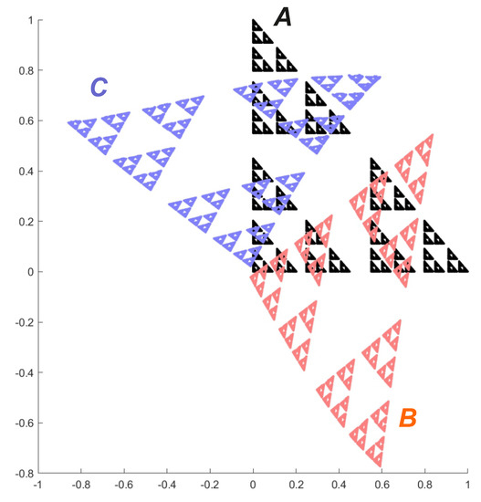
Consider the impulsive pendulum system under a 1-periodic ($\omega =1$) forcing:

$$\left\{\begin{array}{c}{x}^{\prime }=y,y^{\prime }=-sinx+cos2\pi t,t\ne t_j:=j,\hfill \\ (x\left(t_j^{+}\right),y\left(t_j^{+}\right))\in I(x\left(t_j^{-}\right),y\left(t_j^{-}\right)),j\in \mathbb{Z},\hfill \end{array}\right.$$

(22)

where $I:{\mathbb{R}}^2⊸{\mathbb{R}}^2$ is the affine system of disconnected similitudes such that

$$I(x,y):=i_1(x,y)\cup i_2(x,y)\cup i_3(x,y),$$

$$\begin{array}{cc}\hfill i_1(x,y)& =(0.45x,0.45y),\hfill \\ \hfill i_2(x,y)& =(0.45x,0.45y+0.55),\hfill \\ \hfill i_3(x,y)& =(0.45x+0.55,0.45y).\hfill \end{array}$$

The associated Poincaré translation operator $T_1:{\mathbb{R}}^2\to {\mathbb{R}}^2$ takes the form

$$\begin{array}{cc}\hfill T_1(x_0,y_0):=\{& (x\left(1\right),y\left(1\right))\mid (x(·),y(·))isasolutionofthesystem{x}^{\prime }=y,y^{\prime }=-sinx+cos2\pi t\hfill \\ \hfill & suchthat(x\left(0\right),y\left(0\right))=(x_0,y_0)\}.\hfill \end{array}$$

Its inversion $T_1^{-1}:{\mathbb{R}}^2\to {\mathbb{R}}^2$ can be defined as

$$\begin{array}{cc}\hfill T_1^{-1}(x_1,y_1):=\{& (x\left(0\right),y\left(0\right))\mid (x(·),y(·))is\mathrm{a}solutionofthesystem{x}^{\prime }=y,y^{\prime }=-sinx+cos2\pi t\hfill \\ \hfill & suchthat(x\left(1\right),y\left(1\right))=(x_1,y_1)\}.\hfill \end{array}$$

The Sierpiński-like attractor $A=I\left(A\right)$ of the system $\left\{{\mathbb{R}}^2;i_1,i_2,i_3\right\}$, the attractor $B=T_1\left(A\right)$ of the system $\left\{{\mathbb{R}}^2;i_1^{\prime },i_2^{\prime },i_3^{\prime }\right\}$, and the attractor $C=T_1^{-1}\left(A\right)$ of the system $\left\{{\mathbb{R}}^2;i_1^{″},i_2^{″},i_3^{″}\right\}$ are depicted in Figure 1. The fractal (Hausdorff) dimension D of the attractors $A,B,C$ can be easily calculated as

$$D=dimA=dimB=dimC=\frac{log3}{log\frac{1}{0.45}}\doteq 1.376.$$

Remark 15.

The meaning of the illustrative Example 4 can be better understood by means of the following commutative diagrams ($m=3$, $\omega =1$):where $x^{+},x_1^{+},\dots ,x_m^{+}$ are the solutions of (22) such that $x^{+}\left(0\right)$, $x_1^{+}\left(0\right),\dots ,x_m^{+}\left(0\right)\in A$ and $x^{+}\left(\omega \right),x_1^{+}\left(\omega \right),\dots ,x_m^{+}\left(\omega \right)\in B$, while $x^{-},x_1^{-},\dots ,x_m^{-}$ are the solutions of (22) such that $x^{-}\left(0\right),x_1^{-}\left(0\right),\dots ,x_m^{-}\left(0\right)\in C$ and $x^{-}\left(\omega \right),x_1^{-}\left(\omega \right),\dots ,x_m^{-}\left(\omega \right)\in A$. The attractors A, $B=T_{\omega }\left(A\right)$, $C={T_{\omega }}^{-1}\left(A\right)$ such that $A=I\left(A\right)$, $B=I^{\prime }\left(B\right)$, $C=I^{″}\left(C\right)$ are depicted in Figure 1.

Now, consider (13) with the same assumptions as above and suppose additionally that $i_k:{\mathbb{R}}^n\to {\mathbb{R}}^n$ in (20) are contractions such that the sets $i_k\left(A\right)$ are totally disconnected, for all $k=1,\dots ,m$ (see (7)), where $A\in K\left({\mathbb{R}}^n\right)$ is a unique global attractor of the iterated function system $\left\{{\mathbb{R}}^n;i_1,\dots ,i_m\right\}$ guaranteed by Proposition 1. Let $T_{\omega }:{\mathbb{R}}^n\to {\mathbb{R}}^n$ be the Poincaré translation operator along the trajectories of (11), defined in (12). Then we can define the shift dynamical systems $(B,S_1)$ and $(C,S_2)$, associated with the systems $\left\{B;i_1^{\prime }{|}_B,\dots ,i_m^{\prime }{|}_B\right\}$ and $\left\{C;i_1^{″}{|}_C,\dots ,i_m^{″}{|}_C\right\}$, defined in Theorem 5, where $B:=T_{\omega }\left(A\right)$ and $C:={T_{\omega }}^{-1}\left(A\right)$.

Concretely, $S_1:B\to B$ is a single-valued continuous mapping such that

$$S_1\left(b\right):=\bigcup _{k=1}^m{i^{\prime }}_k^{-1}\left(b\right)$$

and $S_1\left(b\right):=i_k^{\prime -1}\left(b\right)=T_{\omega }\circ i_k^{-1}\circ {T_{\omega }}^{-1}\left(b\right)$, provided $b\in i_k^{\prime }\left(B\right)$, $k=1,\dots ,m$. Respectively, $S_2:C\to C$ is a single-valued continuous mapping such that

$$S_2\left(c\right):=\bigcup _{k=1}^m{i}_k^{″-1}\left(c\right)$$

and $S_2\left(c\right):=i_k^{″-1}\left(c\right)={T_{\omega }}^{-1}\circ i_k^{-1}\circ T_{\omega }\left(c\right)$, provided $c\in i_k^{″}\left(C\right)$, $k=1,\dots ,m$.

Theorem 6.

The shift dynamical systems $(B,S_1)$ and $(C,S_2)$ are chaotic in the sense of Devaney (cf. Section 4). The same is true for the induced hypersystems $(K\left(B\right),S_1^{*})$ and $(K\left(C\right),S_2^{*})$ in the hyperspaces $(K\left(B\right),d_H)$ and $(K\left(C\right),d_H)$, where $S_1^{*}\left(\mathcal{B}\right):={\bigcup }_{b\in \mathcal{B}}{S}_1\left(b\right)$ and $S_2^{*}\left(\mathcal{C}\right):={\bigcup }_{c\in \mathcal{C}}{S}_2\left(c\right)$.

Proof. 

According to Theorem 5, B and C are unique global compact attractors of the respective systems $\left\{{\mathbb{R}}^n;i_1^{\prime },\dots ,i_m^{\prime }\right\}$ and $\left\{{\mathbb{R}}^n;i_1^{″},\dots ,i_m^{″}\right\}$. Thus, $I^{\prime }{|}_B:B⊸B$ and $I^{″}{|}_C:C⊸C$, and we can restrict ourselves to the systems $\left\{B;i_1^{\prime }{|}_B,\dots ,i_m^{\prime }{|}_B\right\}$ and $\left\{C;i_1^{″}-.1ex{|}_C,\dots ,i_m^{″}{|}_C\right\}$.

Since $i_k^{-1}:A\to A$ were shown in Section 4 to be injective and invertible, and so single-valued and continuous, the latter must be true for $i_k^{\prime -1}=T_{\omega }\circ i_k^{-1}\circ {T_{\omega }}^{-1}$ as well as $i_k^{″-1}={T_{\omega }}^{-1}\circ i_k^{-1}\circ T_{\omega }$, for all $k=1,\dots ,m$.

Furthermore, since the sets $i_k^{\prime }\left(B\right)$ and $i_k^{″}\left(C\right)$ must be also totally disconnected, the single-valued continuous Hutchinson-Barnsley operators $S_1:B\to B$ and $S_2:C\to C$ can be uniquely defined by

$$S_1\left(b\right):=i_k^{\prime -1}\left(b\right)=T_{\omega }\circ i_k^{-1}\circ {T_{\omega }}^{-1}\left(b\right),\mathrm{provided}b\in i_k^{\prime }\left(B\right),$$

and

$$S_2\left(c\right):=i_k^{″-1}\left(c\right)={T_{\omega }}^{-1}\circ i_k^{-1}\circ T_{\omega }\left(c\right),\mathrm{provided}c\in i_k^{″}\left(C\right),$$

for all $k=1,\dots ,m$.

Since Devaney’s chaos is well known to be a topological invariant (i.e., an invariant under a topological conjugacy) on a compact metric space (see e.g., Reference [64]), the both systems $(B,S_1)$ and $(C,S_2)$ must be chaotic in the sense of Devaney, because the same was recalled to be true for the system $(A,i_1^{-1},\dots ,i_m^{-1})$ in Section 4.

Since the induced maps $S_1^{*}:K\left(B\right)\to K\left(B\right)$ and $S_2^{*}:K\left(C\right)\to K\left(C\right)$ in the hyperspaces $(K\left(B\right),d_H)$ and $(K\left(C\right),d_H)$, where

$$S_1^{*}\left(\mathcal{B}\right):=\bigcup _{b\in \mathcal{B}}{S}_1\left(b\right),\mathcal{B}\in K\left(B\right),\mathrm{and}{S}_2^{*}\left(\mathcal{C}\right):=\bigcup _{c\in \mathcal{C}}{S}_2\left(c\right),\mathcal{C}\in K\left(C\right),$$

are single-valued continuous, because so are the maps $S_1:B\to B$ and $S_2:C\to C$ (see Reference [53]), we can also consider the shift dynamical hypersystems $(K\left(B\right),S_1^{*})$ and $(K\left(C\right),S_2^{*})$.

Since the induced Poincaré operators ${T_{\omega }}^{*}:K\left({\mathbb{R}}^n\right)\to K\left({\mathbb{R}}^n\right)$ remain homeomorphisms and $S_1^{*}={T_{\omega }}^{*}\circ {\left(i_k^{-1}\right)}^{*}\circ {\left({T_{\omega }}^{-1}\right)}^{*}$, $S_2^{*}={\left({T_{\omega }}^{-1}\right)}^{*}\circ {\left(i_k^{-1}\right)}^{*}\circ {T_{\omega }}^{*}$, the hypersystems $(K\left(B\right),S_1^{*})$ and $(K\left(C\right),S_2^{*})$ must be by the same arguments in Reference [64], in view of the last part of Proposition 2, chaotic in the sense of Devaney, too. □

Remark 16.

It is well known that the density of periodic points in the basic space implies the one for induced maps in hyperspaces (see e.g., Reference [30]). Therefore, since the transitivity together with density of periodic points imply a sensitive dependence on initial conditions (i.e., (ii), (iii) ⇒ (i), for the conditions in the definition of Devaney’s chaos in Section 4), provided the basic space is infinite (see again e.g., Reference [30]), we would have to restrict ourselves to transitivity in the alternative proof of Devaney’s chaos for the hypersystems $(K\left(B\right),S_1^{*})$ and $(K\left(C\right),S_2^{*})$. The transitivity in hyperspaces is however not implied in general by the one in the original basic space (see Reference [30]).

Example 5

(continued Example 4). Consider again systems (22). In order to apply Theorem 6, let us define the shift dynamical system $(B,S_1)$ and $(C,S_2)$, where $B=T_1\left(A\right)$, $C=T_1^{-1}\left(A\right)$, $A=I\left(A\right)$,

$$S_1\left(b\right):=\left\{\begin{array}{c}{T}_1\circ \left(\frac{x}{0.45},\frac{y}{0.45}\right)\circ T_1^{-1}\left(b\right),forb\in i_1^{\prime }\left(B\right),\hfill \\ T_1\circ \left(\frac{x}{0.45},\frac{y-0.55}{0.45}\right)\circ T_1^{-1}\left(b\right),forb\in i_2^{\prime }\left(B\right),\hfill \\ T_1\circ \left(\frac{x-0.55}{0.45},\frac{y}{0.45}\right)\circ T_1^{-1}\left(b\right),forb\in i_3^{\prime }\left(B\right),\hfill \end{array}\right.$$

and

$$S_2\left(c\right):=\left\{\begin{array}{c}{T}_1^{-1}\circ \left(\frac{x}{0.45},\frac{y}{0.45}\right)\circ T_1\left(c\right),forc\in i_1^{″}\left(B\right),\hfill \\ T_1^{-1}\circ \left(\frac{x}{0.45},\frac{y-0.55}{0.45}\right)\circ T_1\left(c\right),forc\in i_2^{″}\left(B\right),\hfill \\ T_1^{-1}\circ \left(\frac{x-0.55}{0.45},\frac{y}{0.45}\right)\circ T_1\left(c\right),forc\in i_3^{″}\left(B\right).\hfill \end{array}\right.$$

The shift dynamical systems $(B,S_1)$ and $(C,S_2)$ are, according to Theorem 6, chaotic in the sense of Devaney.

The same is true, according to Theorem 6, for the induced hypersystems $(K\left(B\right),S_1^{*})$ and $(K\left(C\right),S_2^{*})$, where $S_1^{*}\left(\mathcal{B}\right):={\bigcup }_{b\in \mathcal{B}}{S}_1\left(b\right)$ and $S_1^{*}\left(\mathcal{C}\right):={\bigcup }_{c\in \mathcal{C}}{S}_2\left(c\right)$.

8. Concluding Remarks

As already pointed out in the Introduction, no Nielsen periodic point theory so far exists for n-valued maps. In case of any progress for at least $n=2$, we could think about multiple subharmonic (i.e., $k\omega$-periodic with $k>1$) solutions of impulsive differential equations.

If a uniqueness condition is omitted at given (impulsive) differential equations or, more generally, at (impulsive) differential inclusions, then the associated Poincaré translation operators become multivalued and, in particular, admissible in the sense of Górniewicz (see Reference [26]). Then, however, the needed information about their compositions with n-valued impulsive maps would be lost or, even worse, useless. On the other hand, in the splitting case, their compositions with single-valued selections might be useful for at least partial answers. As a starting point, one can therefore study the same problems as above for differential inclusions with single-valued impulses, as indicated e.g., in Reference [19].

Another problem is to randomize at least some obtained results or to extend some random results like those in References [15,65] along the lines discussed above. Unfortunately, the randomization technique which we have to our disposal (see e.g., Reference [15], and the references therein) is based on the existence of measurable selections whose multiplicity can be lost. In other words, no Nielsen theory so far exists for random fixed points.

A more promissible situation concerning a possible extension and application of the obtained results seems to be for the Hutchinson-Barnsley operators (see Remark 7). The appropriate application can be possible, for instance, for a fractal image compression of pictures. The results might be also randomized.

References

- Bainov, D.; Simeonov, P. Impulsive Differential Equations: Periodic Solutions and Applications; Pitman Monographs and Surveys in Pure and Applied Mathematics; Longman Scientific&Technical: Marlow, UK, 1993; Volume 66. [Google Scholar]
- Perestyuk, N.A.; Plotnikov, V.A.; Somoilenko, A.M.; Skripnik, N.V. Differential Equations with Impulsive Effects. Multivalued Right-hand Sides with Discontinuities; De Gruyter Studies in Mathematics; De Gruyter: Berlin, Germany, 2011; Volume 40. [Google Scholar]
- Samoilenko, A.M.; Stanzhytskyi, O. Qualitative and Asymptotic Analysis of Differential Equations with Random Perturbations; World Scientific Series on Nonlinear Science Series A; World Scientific Publishing: Singapore, 2011; Volume 78. [Google Scholar]
- Song, X.; Gno, H.; Shi, X. Theory and Applications of Impulsive Differential Equations; Science Press: Beijing, China, 2011. [Google Scholar]
- Dishlieva, K. Impulsive differential equations and applications. J. Appl. Comput. Math. 2012, 1, 1–3. [Google Scholar] [CrossRef]
- Li, X.; Bohner, M.; Wang, C.K. Impulsive differential equations: Periodic solutions and applications. Automatica 2015, 52, 173–178. [Google Scholar] [CrossRef]
- Church, K.E.; Smith, R.J. Comparing malaria surveillance with periodic spraying in the presence of insecticide-resistant mosquitoes: Should we spray regularly or based on human infections? Math. Biosci. 2016, 276, 145–163. [Google Scholar] [CrossRef] [PubMed]
- Miron, R.E.; Smith, R.J. Modelling imperfect adherence to HIV induction therapy. BMC Infect. Dis. 2010, 10, 6. [Google Scholar] [CrossRef]
- Smith, R.J.; Wolkowicz, G.S.K. Analysis of a model of the nutrient driven self-cycling fermentation process. Dyn. Contin. Discret. Impuls. Syst. Ser. B Appl. Algorithms 2004, 11, 239–265. [Google Scholar]
- Wang, S.; Huang, Q. Bifurcation of nontrivial periodic solutions for a food chain Beddington–DeAngelis interference model with impulsive effect. Int. J. Bifurc. Chaos 2018, 28, 1850131. [Google Scholar] [CrossRef]
- Zhang, Q.; Tang, B.; Cheng, T.; Tang, S. Bifurcation analysis of a generalized impulsive Kolmogorov model with applications to pest and disease control. SIAM J. Appl. Math. 2020, 80, 1796–1819. [Google Scholar] [CrossRef]
- Abbas, S.; Benchohra, M. Advanced Functional Evolution Equations and Inclusions; Springer: Berlin, Germany, 2015. [Google Scholar]
- Abada, N.; Agarwal, R.P.; Benchohra, M.; Hammouchi, H. Impulsive demilinear neutral functional differential inclusions with multivalued jumps. Appl. Math. 2011, 56, 227–250. [Google Scholar] [CrossRef][Green Version]
- Andres, J. The standard Sharkovsky cycle coexistence theorem applies to impulsive differential equations: Some notes and beyond. Proc. Am. Math. Soc. 2019, 147, 1497–1509. [Google Scholar] [CrossRef]
- Andres, J. Application of the randomized Sharkovsky-type theorems to random impulsive differential equations and inclusions. J. Dyn. Diff. Equ. 2019, 31, 2127–2144. [Google Scholar] [CrossRef]
- Benedetti, J. An existence result for impulsive functional differential inclusions in Banach spaces. Discuss. Math. Diff. Incl. Control Optim. 2004, 24, 13–30. [Google Scholar] [CrossRef]
- Malyutina, E.V. On control system with multivalued impulses and delay. Izvestiya Instituta Matematiki i Informatiki Udmurtskogo Gosudarstvennogo Universiteta 2012, 1, 92–93. (In Russian) [Google Scholar]
- Ning, H.; Liu, B. Existence and controllability results for infinite delay partial functional differential systems with multi-valued impulses in Banach spaces. Asian-Eur. J. Math. 2010, 3, 631–646. [Google Scholar] [CrossRef]
- Andres, J. Nielsen number, impulsive differential equations and problem of Jean Leray. Topol. Meth. Nonlinear Anal. 2020, in press. [Google Scholar] [CrossRef]
- Brown, R.F.; Deconinck, C.; Dekimpe, K.; Staecker, P.C. Lifting classes for the fixed point theory of n-valued maps. Topol. Appl. 2020, 274. in press. [Google Scholar] [CrossRef]
- Brown, R.F.; Gonçalves, D.L. On the topology of n-valued maps. Adv. Fixed Point Theory 2018, 8, 205–220. [Google Scholar]
- Brown, R.F.; Furi, M.; Górniewicz, L.; Jiang, B. (Eds.) Fixed Point Theory of Multivalued Weighted Maps; Springer: Dordrecht, The Netherlands, 2005. [Google Scholar]
- Hutchinson, J.E. Fractals and self similarity. Indiana Univ. Math. J. 1981, 30, 713–747. [Google Scholar] [CrossRef]
- Barnsley, M.F. Fractals Everywhere; Academic Press: New York, NY, USA, 1988. [Google Scholar]
- Andres, J.; Górniewicz, L. Topological Fixed Point Principles for Boundary Value Problems; Kluwer: Dordrecht, The Netherlands, 2003. [Google Scholar]
- Górniewicz, L. Topological Fixed Point Theory of Multivalued Mappings, 2nd ed.; Springer: Berlin, Germany, 2006. [Google Scholar]
- Brown, R.F. The Lefschetz Fixed Point Theorem; Scott-Foresman and Co.: Glenview, IL, USA, 1971. [Google Scholar]
- Jiang, B. Lectures on Nielsen Fixed Point Theory; Contemporary Mathematics 14; The American Mathematical Society: Providence, RI, USA, 1983. [Google Scholar]
- Andres, J.; Rypka, M. Multivalued fractals and hyperfractals. Int. J. Bifurc. Chaos 2012, 22, 125009. [Google Scholar] [CrossRef]
- Fedeli, A. On chaotic set-valued discrete dynamical systems. Chaos Solitons Fractals 2005, 23, 1381–1384. [Google Scholar] [CrossRef]
- Better, J. Equivariant Nielsen fixed point theory for n-valued maps. Topol. Appl. 2010, 157, 1804–1814. [Google Scholar] [CrossRef][Green Version]
- Better, J. A Wecken theorem for n-valued maps. Topol. Appl. 2012, 159, 3707–3715. [Google Scholar] [CrossRef][Green Version]
- Brown, R.F. Fixed points of n-valued maps of the circle. Bull. Pol. Acad. Sci. Math. 2006, 54, 153–162. [Google Scholar] [CrossRef][Green Version]
- Brown, R.F. The Lefschetz number of an n-valued multimap. J. Fixed Point Theory Appl. 2007, 1, 53–60. [Google Scholar]
- Brown, R.F. Nielsen numbers of n-valued fiber maps. J. Fixed Point Theory Appl. 2008, 2, 183–201. [Google Scholar] [CrossRef][Green Version]
- Brown, R.F. Construction of multiply fixed n-valued maps. Topol. Appl. 2015, 196, 249–259. [Google Scholar] [CrossRef]
- Brown, R.F.; Kolahi, K. Nielsen coincidence, fixed point and root theories of n-valued maps. J. Fixed Point Theory Appl. 2013, 14, 309–324. [Google Scholar] [CrossRef][Green Version]
- Brown, R.F.; Lin, J.T.L.K. Coincidences of projections and linear n-valued maps of tori. Topol. Appl. 2010, 157, 1990–1998. [Google Scholar] [CrossRef][Green Version]
- Brown, R.F.; Nan, J. Stabilizers of fixed point classes and Nielsen numbers of n-valued maps. Bull. Belg. Math. Soc. Adv. Fixed Point Theory 2017, 24, 523–535. [Google Scholar] [CrossRef][Green Version]
- Crabb, M.C. Lefschetz indices for n-valued maps. J. Fixed Point Theory Appl. 2015, 17, 153–186. [Google Scholar] [CrossRef]
- Gonçalves, D.L.; Guaschi, J. Fixed points of n-valued maps on surfaces and the Wecken property—A configuration space approach. Sci. China Math. 2017, 60, 1561–1574. [Google Scholar] [CrossRef]
- Gonçalves, D.L.; Guaschi, J. Fixed points of n-valued maps, the fixed point property and the case of surfaces—A braid approach. Indag. Math. 2018, 29, 91–124. [Google Scholar] [CrossRef]
- Jezierski, J. An example of finitely-valued fixed point free map. Zesz. Nauk (Univ. Grańsk) 1987, 6, 87–93. [Google Scholar]
- O’Neil, B. Induced homology homomorphism for set-valued maps. Pac. J. Math. 1957, 7, 1179–1184. [Google Scholar] [CrossRef]
- Schirmer, H. Fix-finite approximations of n-valued multifunctions. Fund. Math. 1984, 121, 73–80. [Google Scholar] [CrossRef][Green Version]
- Schirmer, H. An index and a Nielsen number for n-valued multifunctions. Fund. Math. 1984, 124, 207–219. [Google Scholar] [CrossRef]
- Schirmer, H. A minimum theorem for n-valued multifunctions. Fund. Math. 1985, 126, 83–92. [Google Scholar] [CrossRef][Green Version]
- Staecker, P.C. Axioms for the fixed point index of n-valued maps, and some applications. J. Fixed Point Theory Appl. 2018, 20, 61. [Google Scholar] [CrossRef]
- Dzedzej, Z. Fixed Point Index Theory for a Class of Nonacyclic Multivalued Maps; Dissertationes Math. 253; PWN: Warsaw, Poland, 1985. [Google Scholar]
- Pejsachowicz, J.; Skiba, R. Fixed Point Theory of Multivalued Weighted Maps. In Handbook of Topological Fixed Point Theory; Brown, R.F., Furi, M., Górniewicz, L., Jiang, B., Eds.; Springer: Dordrecht, The Netherlands, 2005; pp. 217–263. [Google Scholar] [CrossRef]
- Banach, S.; Mazur, S. Über mehrdeutige stetige Abbildungen. Stud. Math. 1934, 5, 174–178. [Google Scholar] [CrossRef]
- Haase, H. Chaotic maps in hyperspaces. Real Anal. Exch. 1995, 21, 689–695. [Google Scholar] [CrossRef]
- Andres, J.; Fišer, J. Metric and topological multivalued fractals. Int. J. Bifurc. Chaos 2004, 14, 1277–1289. [Google Scholar] [CrossRef]
- Andres, J.; Górniewicz, L. Note on nonejective topological fractals on Peano’s continua. Int. J. Bifurc. Chaos 2014, 24, 1450148. [Google Scholar] [CrossRef]
- Andres, J.; Väth, M. Calculation of Lefschetz and Nielsen numbers in hyperspaces for fractals and dynamical systems. Proceed. Am. Math. Soc. 2007, 135, 479–487. [Google Scholar] [CrossRef]
- Krasnoselskii, M.A. The Operator of Translation along the Trajectories of Differential Equations; Translations of Mathematical Monographs; American Mathematical Society: Providence, RI, USA, 1968; Volume 19. [Google Scholar]
- Codington, E.A.; Levinson, N. Theory of Differential Equations; McGraw-Hill: New York, NY, USA, 1985. [Google Scholar]
- Banakh, T.; Nowak, M.; Strobin, F. Detecting topological and Banach fractals among zero-dimensional spaces. Topol. Appl. 2015, 196, 22–30. [Google Scholar] [CrossRef]
- Banakh, T.; Nowak, M.; Strobin, F. Embedding fractals in Banach, Hilbert or Euclidean spaces. J. Fractal Geom. 2018, in press. [Google Scholar]
- Montiel, M.E.; Aguado, A.S.; Zaluska, E. Topology in fractals. Chaos Solitons Fractals 1996, 7, 1187–1207. [Google Scholar] [CrossRef]
- Barnsley, M.F.; Harding, B.; Rypka, M. Measure preserving fractal homeomorphisms. In Fractals, Wavelets, and Their Applications; Bandt, C., Barnsley, M., Devaney, R., Falconer, K.J., Kannan, V., Vinod Kumar, P.B., Eds.; Springer: Cham, Switzerland, 2014; pp. 79–102. [Google Scholar]
- Falconer, K. Fractal Geometry: Mathematical Foundations and Applications; J. Wiley & Sons: New York, NY, USA, 1990. [Google Scholar]
- Falconer, K. Techniques in Fractal Geometry; J. Wiley & Sons: New York, NY, USA, 1997. [Google Scholar]
- Kirchgraber, U.; Hoffer, D. On the definition of chaos. Z. Angew. Math. Mech. 1989, 69, 175–185. [Google Scholar] [CrossRef]
- Shang, Y. Emergence in random noisy environment. Int. J. Math. Anal. 2010, 4, 1205–1215. [Google Scholar]
© 2020 by the author. Licensee MDPI, Basel, Switzerland. This article is an open access article distributed under the terms and conditions of the Creative Commons Attribution (CC BY) license (http://creativecommons.org/licenses/by/4.0/).