Binary Whale Optimization Algorithm for Dimensionality Reduction


Abstract
1. Introduction
2. Whale Optimization Algorithm
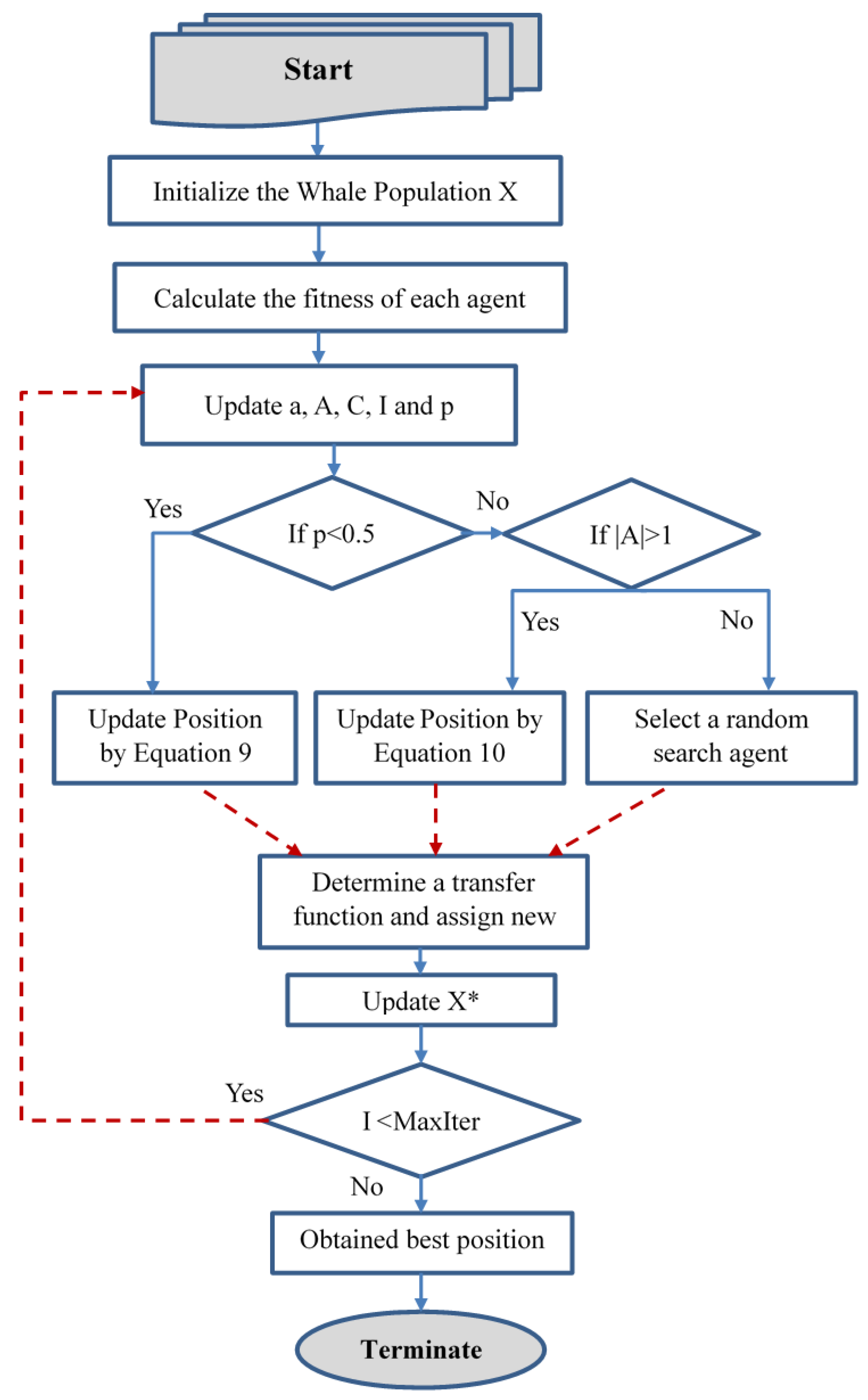
3. Binary Whale Optimization Algorithm
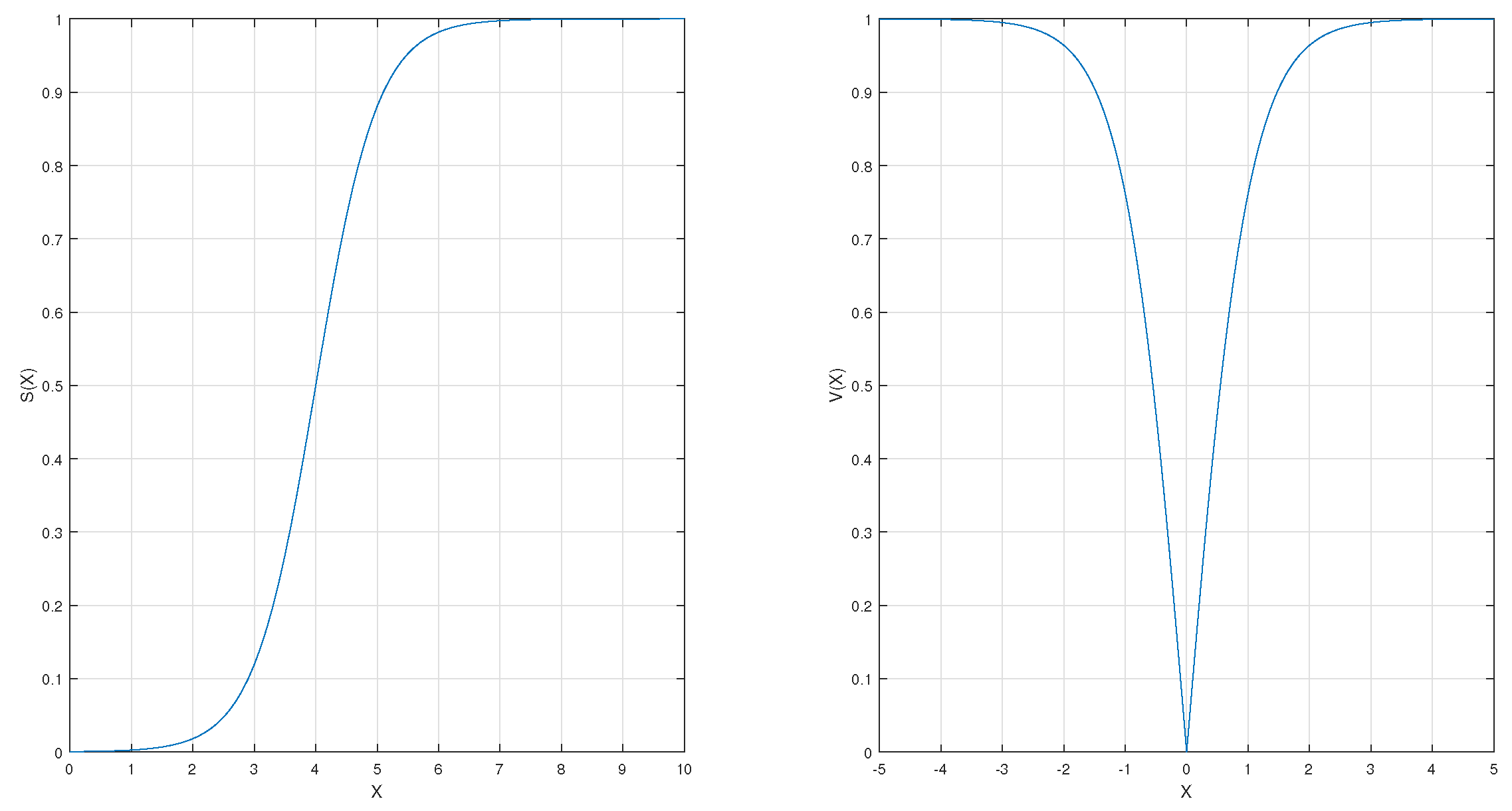
3.1. Approach 1: Proposed bWOA-S
3.2. Approach 2: Proposed bWOA-V
| Algorithm 1 Pseudo code of bWOA-S & bWOA-V |
|
3.3. bWOA-S and bWOA-V for Feature Selection
4. Experimental Results and Discussion
4.1. Data Acquisition
4.2. Evaluation Criteria
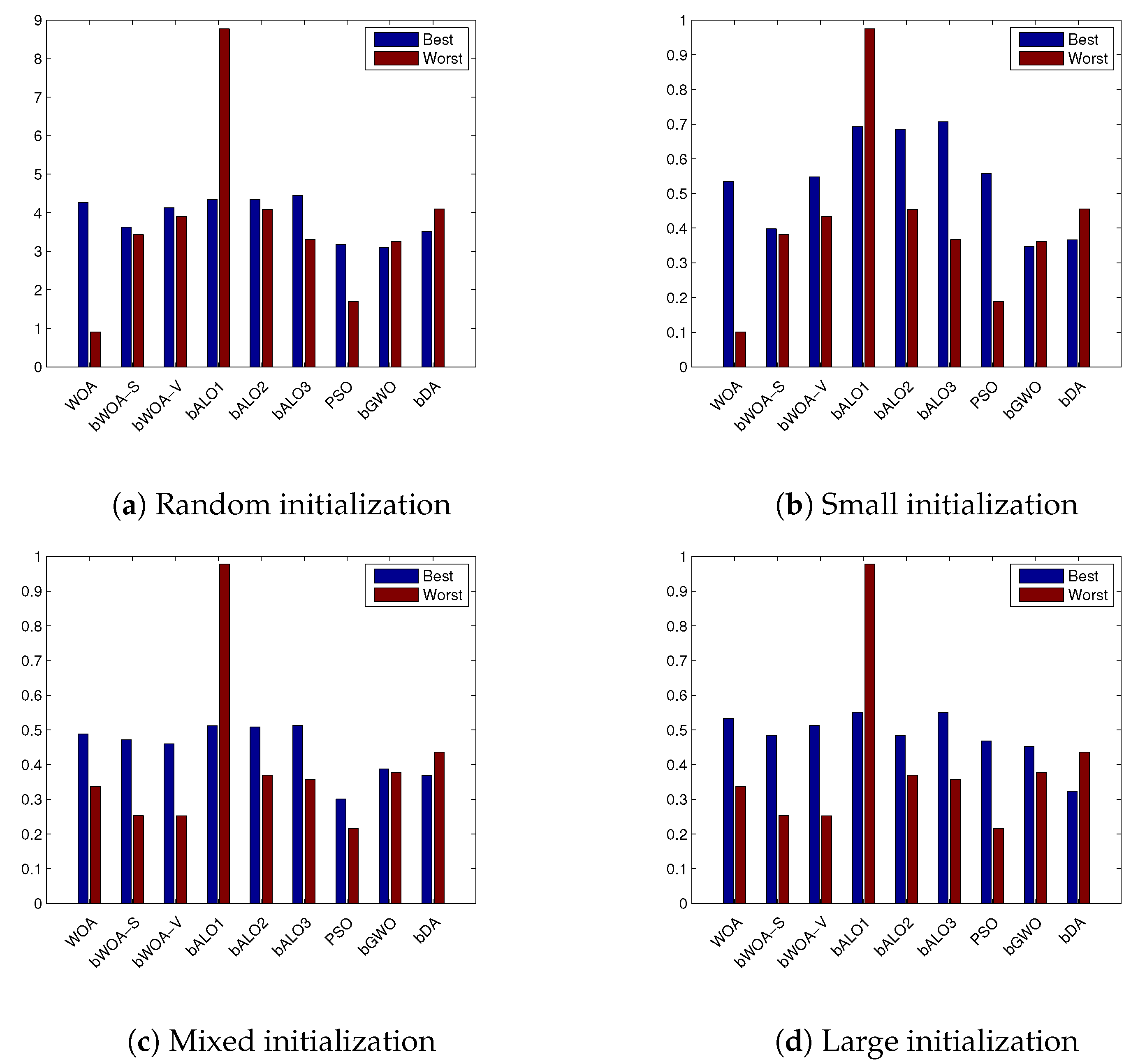
- Best: The minimum (or best for a minimization problem) fitness function value obtained at different independent runs, as depicted in Equation (14).
- Worst: The maximum (or worst for a minimization) fitness function value obtained at different independent operations, as shown in Equation (15).
- Mean: Average calculation performance of the optimization algorithm applied M times, as shown in Equation (16).where is the optimal solution obtained in the i-th operation;
- Standard deviation (Std) can be calculated from the following Equation (17).
- Average classification accuracy: Investigates the accuracy of the classifier and can be calculated by Equation (18).where refers to classifier output for instance i; N refers to the instance number in the test set; and refers to the reference class corresponding to instance i;
- Average selection size (Avg-Selection) measures the average reduction in selected features from all feature sets and is calculated by Equation (19)where is the total number of features in the original dataset;
- Average execution time (Avg-Time) measures the average execution time in milliseconds for all comparison optimization algorithms to obtain the results over the different runs and calculated by Equation (20)where M refers to the run number for the optimizer a, and is the computational time for optimizer a in milliseconds at run number i;
- Wilcoxon rank sum test (Wilcoxon): a non-parametric test called Wilcoxon Rank Sum (WRS) [67]. The test gives ranks to all the scores in one group, and after that the ranks of each group are added. The rank-sum test is often described as the non-parametric version of the t test for two independent groups.
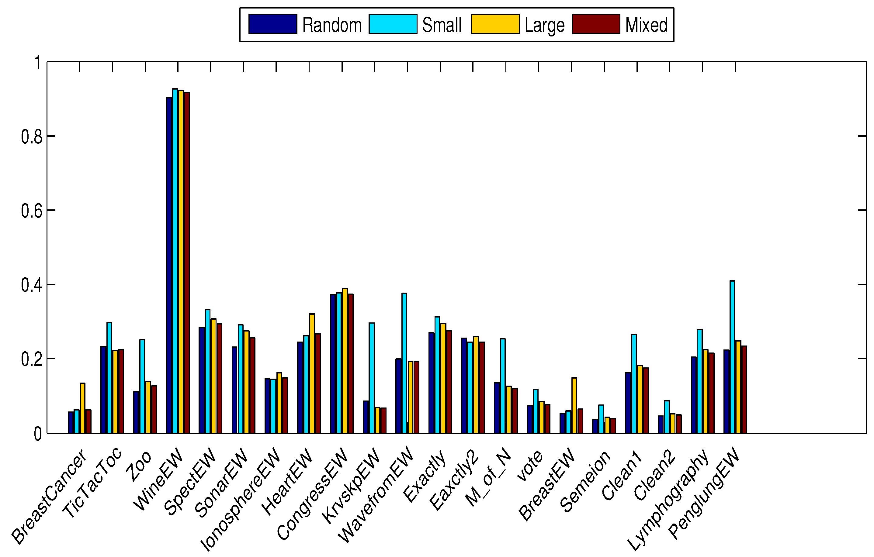
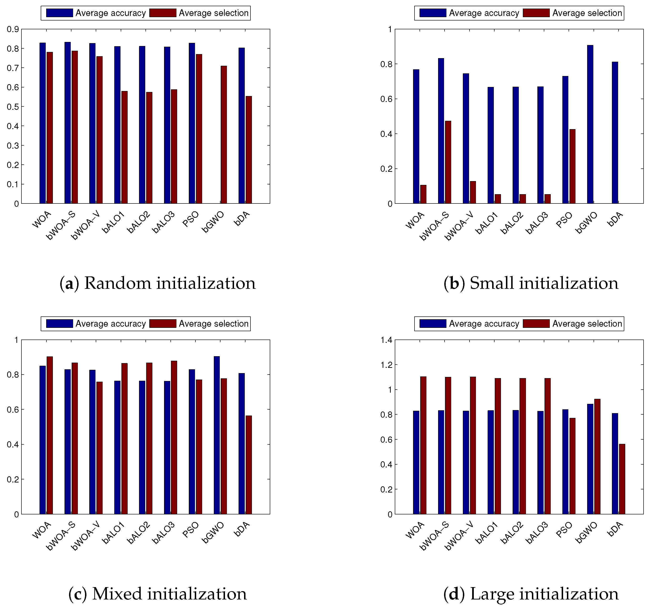
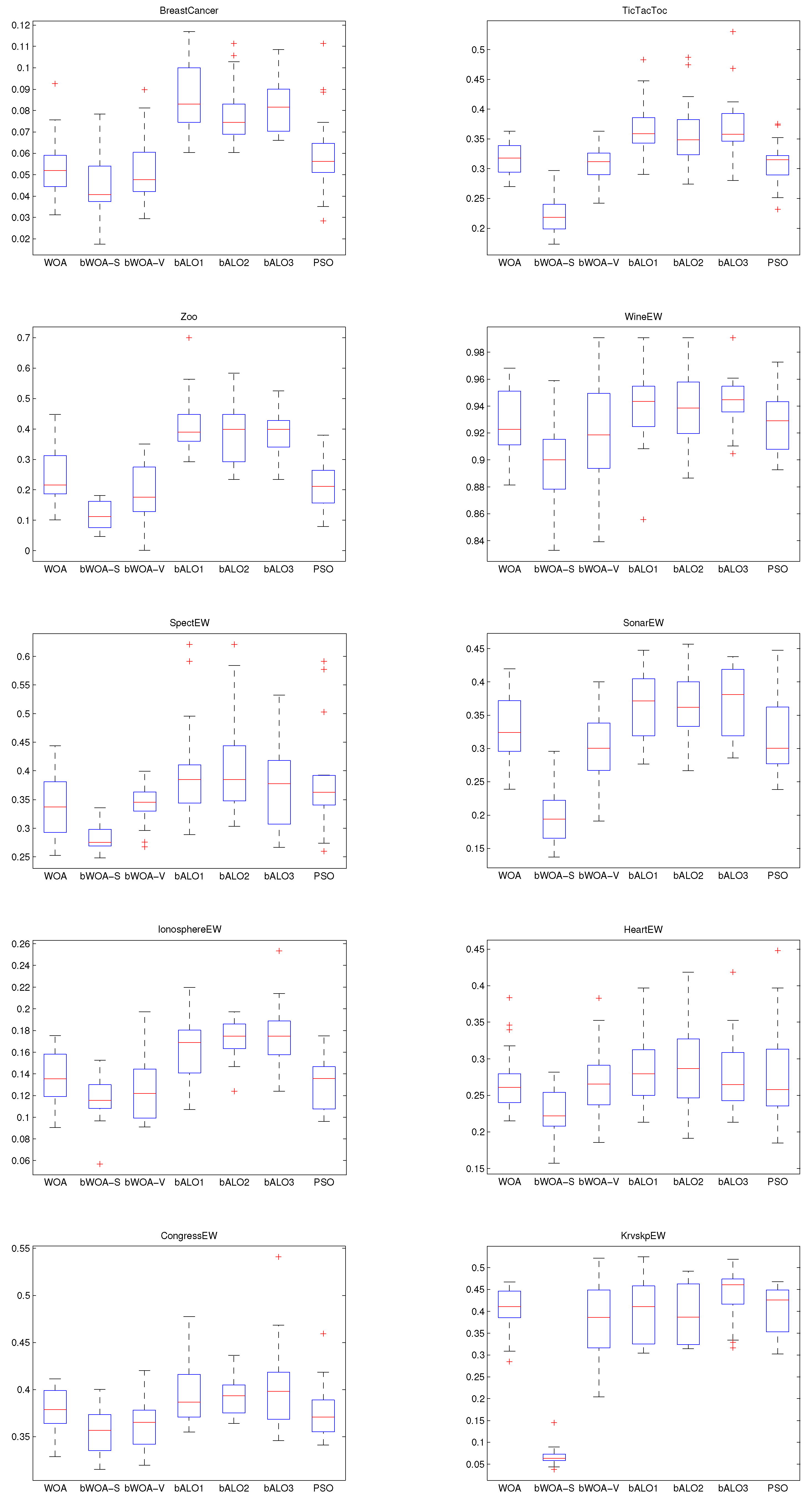
4.3. Performance on Small Initialization
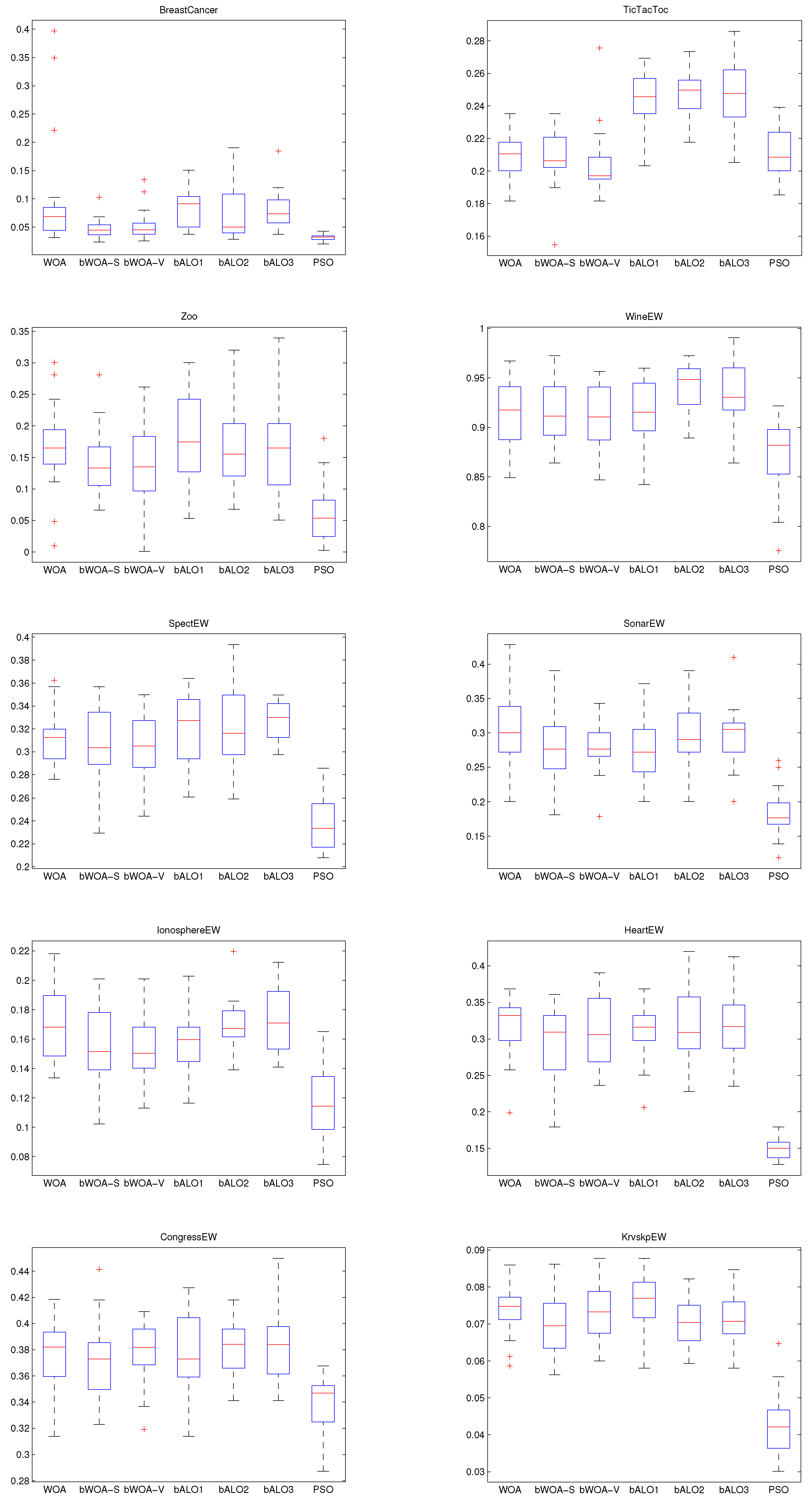
4.4. Performance on Large Initialization
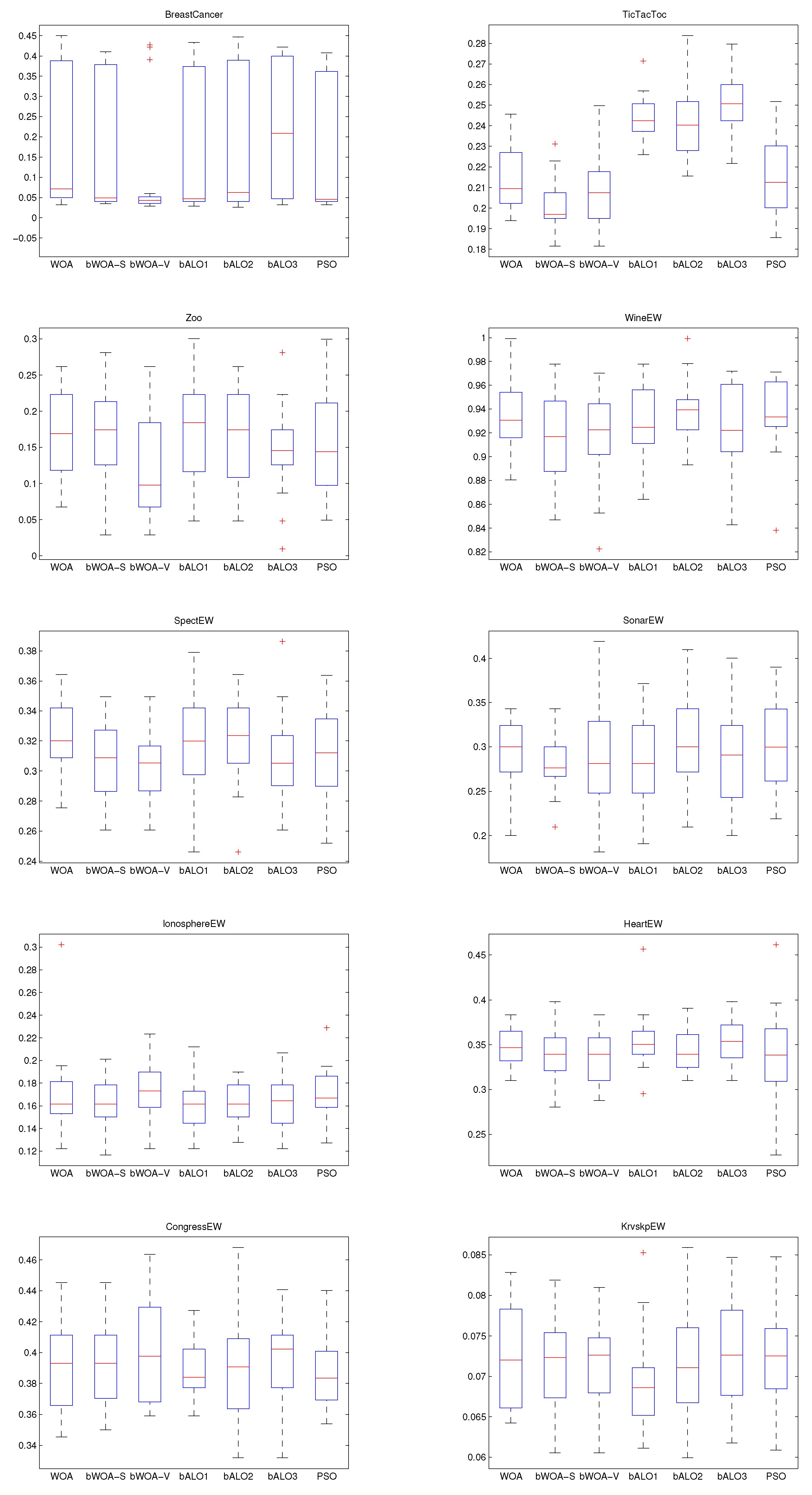
4.5. Performance on Mixed Initialization
4.6. Discussion
5. Conclusions and Future Work
Author Contributions
Funding
Conflicts of Interest
References
- Yi, J.H.; Deb, S.; Dong, J.; Alavi, A.H.; Wang, G.G. An improved NSGA-III algorithm with adaptive mutation operator for Big Data optimization problems. Future Gener. Comput. Syst. 2018, 88, 571–585. [Google Scholar] [CrossRef]
- Neggaz, N.; Houssein, E.H.; Hussain, K. An efficient henry gas solubility optimization for feature selection. Expert Syst. Appl. 2020, 152, 113364. [Google Scholar] [CrossRef]
- Sayed, S.A.F.; Nabil, E.; Badr, A. A binary clonal flower pollination algorithm for feature selection. Pattern Recognit. Lett. 2016, 77, 21–27. [Google Scholar] [CrossRef]
- Martin-Bautista, M.J.; Vila, M.A. A survey of genetic feature selection in mining issues. In Proceedings of the 1999 Congress on Evolutionary Computation-CEC99 (Cat. No. 99TH8406), Washington, DC, USA, 6–9 July 1999; Volume 2, pp. 1314–1321. [Google Scholar]
- Piramuthu, S. Evaluating feature selection methods for learning in data mining applications. Eur. J. Oper. Res. 2004, 156, 483–494. [Google Scholar] [CrossRef]
- Gunal, S.; Edizkan, R. Subspace based feature selection for pattern recognition. Inf. Sci. 2008, 178, 3716–3726. [Google Scholar] [CrossRef]
- Lew, M.S. Principles of Visual Information Retrieval; Springer Science & Business Media: Berlin, Germany, 2013. [Google Scholar]
- Wang, G.G.; Tan, Y. Improving metaheuristic algorithms with information feedback models. IEEE Trans. Cybern. 2017, 49, 542–555. [Google Scholar] [CrossRef] [PubMed]
- Houssein, E.H.; Hosney, M.E.; Elhoseny, M.; Oliva, D.; Mohamed, W.M.; Hassaballah, M. Hybrid Harris hawks optimization with cuckoo search for drug design and discovery in chemoinformatics. Sci. Rep. 2020, 10, 1–22. [Google Scholar] [CrossRef] [PubMed]
- Houssein, E.H.; Hosney, M.E.; Oliva, D.; Mohamed, W.M.; Hassaballah, M. A novel hybrid Harris hawks optimization and support vector machines for drug design and discovery. Comput. Chem. Eng. 2020, 133, 106656. [Google Scholar] [CrossRef]
- Gao, D.; Wang, G.G.; Pedrycz, W. Solving fuzzy job-shop scheduling problem using de algorithm improved by a selection mechanism. IEEE Trans. Fuzzy Syst. 2020. [Google Scholar] [CrossRef]
- Houssein, E.H.; Saad, M.R.; Hussain, K.; Zhu, W.; Shaban, H.; Hassaballah, M. Optimal sink node placement in large scale wireless sensor networks based on Harris’ hawk optimization algorithm. IEEE Access 2020, 8, 19381–19397. [Google Scholar] [CrossRef]
- Ahmed, M.M.; Houssein, E.H.; Hassanien, A.E.; Taha, A.; Hassanien, E. Maximizing lifetime of large-scale wireless sensor networks using multi-objective whale optimization algorithm. Telecommun. Syst. 2019, 72, 243–259. [Google Scholar] [CrossRef]
- Chandrashekar, G.; Sahin, F. A survey on feature selection methods. Comput. Electr. Eng. 2014, 40, 16–28. [Google Scholar] [CrossRef]
- Liu, H.; Yu, L. Toward integrating feature selection algorithms for classification and clustering. IEEE Trans. Knowl. Data Eng. 2005, 17, 491–502. [Google Scholar]
- Kohavi, R.; John, G.H. Wrappers for feature subset selection. Artif. Intell. 1997, 97, 273–324. [Google Scholar] [CrossRef]
- Liu, H.; Setiono, R. A probabilistic approach to feature selection-a filter solution. In Proceedings of the 13th International Conference on Machine Learning, Bari, Italy, 3–6 July 1996; Volume 23, pp. 319–327. [Google Scholar]
- Hastie, T.; Tibshirani, R.; Friedman, J. The Elements of Statistical Learning: Data Mining, Inference, and Prediction; Springer: New York, NY, USA, 2002. [Google Scholar]
- Safavian, S.R.; Landgrebe, D. hastie2002elements. IEEE Trans. Syst. Man, Cybern. 1991, 21, 660–674. [Google Scholar] [CrossRef]
- Dasarathy, B.V. Nearest Neighbor ({NN}) Norms:{NN} Pattern Classification Techniques; IEEE Computer Society Press: Washington, DC, USA, 1991. [Google Scholar]
- Verikas, A.; Bacauskiene, M. Feature selection with neural networks. Pattern Recognit. Lett. 2002, 23, 1323–1335. [Google Scholar] [CrossRef]
- Vapnik, V.N.; Vapnik, V. Statistical Learning Theory; Wiley: New York, NY, USA, 1998; Volume 1. [Google Scholar]
- Khalid, S.; Khalil, T.; Nasreen, S. A survey of feature selection and feature extraction techniques in machine learning. In Proceedings of the Science and Information Conference (SAI), London, UK, 27–29 August 2014; pp. 372–378. [Google Scholar]
- Wang, G.G.; Guo, L.; Gandomi, A.H.; Hao, G.S.; Wang, H. Chaotic krill herd algorithm. Inf. Sci. 2014, 274, 17–34. [Google Scholar] [CrossRef]
- Hassanien, A.E.; Emary, E. Swarm Intelligence: Principles, Advances, and Applications; CRC Press: Boca Raton, FL, USA, 2016. [Google Scholar]
- Mirjalili, S.; Lewis, A. The whale optimization algorithm. Adv. Eng. Softw. 2016, 95, 51–67. [Google Scholar] [CrossRef]
- Hussien, A.G.; Amin, M.; Abd El Aziz, M. A comprehensive review of moth-flame optimisation: Variants, hybrids, and applications. J. Exp. Theor. Artif. Intell. 2020, 32, 705–725. [Google Scholar] [CrossRef]
- Assiri, A.S.; Hussien, A.G.; Amin, M. Ant Lion Optimization: Variants, hybrids, and applications. IEEE Access 2020, 8, 77746–77764. [Google Scholar] [CrossRef]
- Hussien, A.G.; Amin, M.; Wang, M.; Liang, G.; Alsanad, A.; Gumaei, A.; Chen, H. Crow Search Algorithm: Theory, Recent Advances, and Applications. IEEE Access 2020, 8, 173548–173565. [Google Scholar] [CrossRef]
- Shareef, H.; Ibrahim, A.A.; Mutlag, A.H. Lightning search algorithm. Appl. Soft Comput. 2015, 36, 315–333. [Google Scholar] [CrossRef]
- Hashim, F.A.; Houssein, E.H.; Mabrouk, M.S.; Al-Atabany, W.; Mirjalili, S. Henry gas solubility optimization: A novel physics-based algorithm. Future Gener. Comput. Syst. 2019, 101, 646–667. [Google Scholar] [CrossRef]
- Houssein, E.H.; Saad, M.R.; Hashim, F.A.; Shaban, H.; Hassaballah, M. Lévy flight distribution: A new metaheuristic algorithm for solving engineering optimization problems. Eng. Appl. Artif. Intell. 2020, 94, 103731. [Google Scholar] [CrossRef]
- Hashim, F.A.; Houssein, E.H.; Hussain, K.; Mabrouk, M.S.; Al-Atabany, W. A modified Henry gas solubility optimization for solving motif discovery problem. Neural Comput. Appl. 2020, 32, 10759–10771. [Google Scholar] [CrossRef]
- Fernandes, C.; Pontes, A.; Viana, J.; Gaspar-Cunha, A. Using multiobjective evolutionary algorithms in the optimization of operating conditions of polymer injection molding. Polym. Eng. Sci. 2010, 50, 1667–1678. [Google Scholar] [CrossRef]
- Gaspar-Cunha, A.; Covas, J.A. RPSGAe—Reduced Pareto set genetic algorithm: Application to polymer extrusion. In Metaheuristics for Multiobjective Optimisation; Springer: Berlin/Heidelberg, Germany, 2004; pp. 221–249. [Google Scholar]
- Avalos, O.; Cuevas, E.; Gálvez, J.; Houssein, E.H.; Hussain, K. Comparison of Circular Symmetric Low-Pass Digital IIR Filter Design Using Evolutionary Computation Techniques. Mathematics 2020, 8, 1226. [Google Scholar] [CrossRef]
- Xue, B.; Zhang, M.; Browne, W.N.; Yao, X. A survey on evolutionary computation approaches to feature selection. IEEE Trans. Evol. Comput. 2016, 20, 606–626. [Google Scholar] [CrossRef]
- Kabir, M.M.; Shahjahan, M.; Murase, K. A new hybrid ant colony optimization algorithm for feature selection. Expert Syst. Appl. 2012, 39, 3747–3763. [Google Scholar] [CrossRef]
- Ghaemi, M.; Feizi-Derakhshi, M.R. Feature selection using forest optimization algorithm. Pattern Recognit. 2016, 60, 121–129. [Google Scholar] [CrossRef]
- Emary, E.; Zawbaa, H.M.; Ghany, K.K.A.; Hassanien, A.E.; Parv, B. Firefly optimization algorithm for feature selection. In Proceedings of the 7th Balkan Conference on Informatics Conference, Craiova, Romania, 2–4 September 2015; p. 26. [Google Scholar]
- Mafarja, M.M.; Mirjalili, S. Hybrid Whale Optimization Algorithm with simulated annealing for feature selection. Neurocomputing 2017, 260, 302–312. [Google Scholar] [CrossRef]
- Xue, B.; Zhang, M.; Browne, W.N. Particle swarm optimization for feature selection in classification: A multi-objective approach. IEEE Trans. Cybern. 2013, 43, 1656–1671. [Google Scholar] [CrossRef]
- Hafez, A.I.; Zawbaa, H.M.; Emary, E.; Hassanien, A.E. Sine cosine optimization algorithm for feature selection. In Proceedings of the 2016 International Symposium on INnovations in Intelligent Systems and Applications (INISTA), Sinaia, Romania, 2–5 August 2016; pp. 1–5. [Google Scholar]
- Wang, G.G.; Deb, S.; Cui, Z. Monarch butterfly optimization. Neural Comput. Appl. 2019, 31, 1995–2014. [Google Scholar] [CrossRef]
- Wang, G.G. Moth search algorithm: A bio-inspired metaheuristic algorithm for global optimization problems. Memetic Comput. 2018, 10, 151–164. [Google Scholar] [CrossRef]
- Rodrigues, D.; Yang, X.S.; De Souza, A.N.; Papa, J.P. Binary flower pollination algorithm and its application to feature selection. In Recent Advances in Swarm Intelligence and Evolutionary Computation; Springer: Berlin/Heidelberg, Germany, 2015; pp. 85–100. [Google Scholar]
- Nakamura, R.Y.; Pereira, L.A.; Costa, K.; Rodrigues, D.; Papa, J.P.; Yang, X.S. BBA: A binary bat algorithm for feature selection. In Proceedings of the 2012 25th SIBGRAPI Conference on Graphics, Patterns and Images (SIBGRAPI), Ouro Preto, Brazil, 22–25 August 2012; pp. 291–297. [Google Scholar]
- Rodrigues, D.; Pereira, L.A.; Almeida, T.; Papa, J.P.; Souza, A.; Ramos, C.C.; Yang, X.S. BCS: A binary cuckoo search algorithm for feature selection. In Proceedings of the 2013 IEEE International Symposium on Circuits and Systems (ISCAS), Beijing, China, 19–23 May 2013; pp. 465–468. [Google Scholar]
- He, X.; Zhang, Q.; Sun, N.; Dong, Y. Feature selection with discrete binary differential evolution. In Proceedings of the 2009 International Conference on Artificial Intelligence and Computational Intelligence, Shanghai, China, 7–8 November 2009; Volume 4, pp. 327–330. [Google Scholar]
- Emary, E.; Zawbaa, H.M.; Hassanien, A.E. Binary ant lion approaches for feature selection. Neurocomputing 2016, 213, 54–65. [Google Scholar] [CrossRef]
- Emary, E.; Zawbaa, H.M.; Hassanien, A.E. Binary grey wolf optimization approaches for feature selection. Neurocomputing 2016, 172, 371–381. [Google Scholar] [CrossRef]
- Rashedi, E.; Nezamabadi-Pour, H.; Saryazdi, S. BGSA: Binary gravitational search algorithm. Nat. Comput. 2010, 9, 727–745. [Google Scholar] [CrossRef]
- Hussien, A.G.; Hassanien, A.E.; Houssein, E.H. Swarming behaviour of salps algorithm for predicting chemical compound activities. In Proceedings of the 2017 Eighth International Conference on Intelligent Computing and Information Systems (ICICIS), Cairo, Egypt, 5–7 December 2017; pp. 315–320. [Google Scholar]
- Nezamabadi-pour, H.; Rostami-Shahrbabaki, M.; Maghfoori-Farsangi, M. Binary particle swarm optimization: Challenges and new solutions. CSI J. Comput. Sci. Eng. 2008, 6, 21–32. [Google Scholar]
- Hussien, A.G.; Houssein, E.H.; Hassanien, A.E. A binary whale optimization algorithm with hyperbolic tangent fitness function for feature selection. In Proceedings of the 2017 Eighth International Conference on Intelligent Computing and Information Systems (ICICIS), Cairo, Egypt, 5–7 December 2017; pp. 166–172. [Google Scholar]
- Hussien, A.G.; Hassanien, A.E.; Houssein, E.H.; Bhattacharyya, S.; Amin, M. S-shaped Binary Whale Optimization Algorithm for Feature Selection. In Recent Trends in Signal and Image Processing; Springer: Berlin/Heidelberg, Germany, 2019; pp. 79–87. [Google Scholar]
- Hussien, A.G.; Hassanien, A.E.; Houssein, E.H.; Amin, M.; Azar, A.T. New binary whale optimization algorithm for discrete optimization problems. Eng. Optim. 2020, 52, 945–959. [Google Scholar] [CrossRef]
- Chuang, L.Y.; Chang, H.W.; Tu, C.J.; Yang, C.H. Improved binary PSO for feature selection using gene expression data. Comput. Biol. Chem. 2008, 32, 29–38. [Google Scholar] [CrossRef]
- Dua, D.; Graff, C. UCI Machine Learning Repository. 2017. Available online: http://archive.ics.uci.edu/ml (accessed on 28 September 2020).
- Eberhart, R.; Kennedy, J. A new optimizer using particle swarm theory. In Proceedings of the Sixth International Symposium on Micro Machine and Human Science, Nagoya, Japan, 4–6 October 1995; pp. 39–43. [Google Scholar]
- Mafarja, M.M.; Eleyan, D.; Jaber, I.; Hammouri, A.; Mirjalili, S. Binary dragonfly algorithm for feature selection. In Proceedings of the 2017 International Conference on New Trends in Computing Sciences (ICTCS), Amman, Jordan, 11–13 October 2017; pp. 12–17. [Google Scholar]
- D’Angelo, G.; Palmieri, F. GGA: A modified Genetic Algorithm with Gradient-based Local Search for Solving Constrained Optimization Problems. Inf. Sci. 2020, 547, 136–162. [Google Scholar] [CrossRef]
- Mirjalili, S.; Hashim, S.Z.M. BMOA: Binary magnetic optimization algorithm. Int. J. Mach. Learn. Comput. 2012, 2, 204. [Google Scholar] [CrossRef]
- Alon, U.; Barkai, N.; Notterman, D.A.; Gish, K.; Ybarra, S.; Mack, D.; Levine, A.J. Broad patterns of gene expression revealed by clustering analysis of tumor and normal colon tissues probed by oligonucleotide arrays. Proc. Natl. Acad. Sci. USA 1999, 96, 6745–6750. [Google Scholar] [CrossRef] [PubMed]
- Alizadeh, A.A.; Eisen, M.B.; Davis, R.E.; Ma, C.; Lossos, I.S.; Rosenwald, A.; Boldrick, J.C.; Sabet, H.; Tran, T.; Yu, X.; et al. Distinct types of diffuse large B-cell lymphoma identified by gene expression profiling. Nature 2000, 403, 503–511. [Google Scholar] [CrossRef] [PubMed]
- Golub, T.R.; Slonim, D.K.; Tamayo, P.; Huard, C.; Gaasenbeek, M.; Mesirov, J.P.; Coller, H.; Loh, M.L.; Downing, J.R.; Caligiuri, M.A.; et al. Molecular classification of cancer: Class discovery and class prediction by gene expression monitoring. Science 1999, 286, 531–537. [Google Scholar] [CrossRef] [PubMed]
- Wilcoxon, F. Individual comparisons by ranking methods. Biom. Bull. 1945, 1, 80–83. [Google Scholar] [CrossRef]


| Parameter | Value |
|---|---|
| No of search agents | 8 |
| No of iterations | 70 |
| Problem dimension | No. of features in the data |
| Data Search domain | [0, 1] |
| No. repetitions of runs | 20 |
| Inertia factor of PSO | 0.1 |
| Individual-best acceleration factor of PSO | 0.1 |
| Parameter in the fitness function | 0.99 |
| Parameter in the fitness function | 0.01 |
| No. | Name | Features | Samples |
|---|---|---|---|
| 1 | Breastcancer | 9 | 699 |
| 2 | Tic-tac-toe | 9 | 958 |
| 3 | Zoo | 16 | 101 |
| 4 | WineEW | 13 | 178 |
| 5 | SpectEW | 22 | 267 |
| 6 | SonarEW | 60 | 208 |
| 7 | IonosphereEW | 34 | 351 |
| 8 | HeartEW | 13 | 270 |
| 9 | CongressEW | 16 | 435 |
| 10 | KrvskpEW | 36 | 3196 |
| 11 | WaveformEW | 40 | 5000 |
| 12 | Exactly | 13 | 1000 |
| 13 | Exactly 2 | 13 | 1000 |
| 14 | M-of-N | 13 | 1000 |
| 15 | vote | 16 | 300 |
| 16 | BreastEW | 30 | 569 |
| 17 | Semeion | 265 | 1593 |
| 18 | Clean 1 | 166 | 476 |
| 19 | Clean 2 | 166 | 6598 |
| 20 | Lymphography | 18 | 148 |
| 21 | PenghungEW | 325 | 73 |
| 22 | Colon | 2000 | 62 |
| 23 | lymphoma | 96 | 4026 |
| 24 | Leukemia | 7129 | 72 |
| No. | WOA | bWOA-S | bWOA-v | BALO1 | BALO2 | BALO3 | PSO | bGWO | bDA |
|---|---|---|---|---|---|---|---|---|---|
| 1 | 0.061 | 0.049 | 0.051 | 0.079 | 0.095 | 0.088 | 0.060 | 0.035 | 0.031 |
| 2 | 0.327 | 0.224 | 0.313 | 0.345 | 0.352 | 0.334 | 0.333 | 0.243 | 0.210 |
| 3 | 0.247 | 0.133 | 0.220 | 0.411 | 0.395 | 0.416 | 0.249 | 0.127 | 0.058 |
| 4 | 0.933 | 0.908 | 0.937 | 0.955 | 0.960 | 0.953 | 0.926 | 0.880 | 0.877 |
| 5 | 0.345 | 0.295 | 0.340 | 0.351 | 0.391 | 0.375 | 0.362 | 0.276 | 0.253 |
| 6 | 0.337 | 0.203 | 0.315 | 0.374 | 0.372 | 0.369 | 0.303 | 0.154 | 0.188 |
| 7 | 0.137 | 0.123 | 0.131 | 0.175 | 0.177 | 0.184 | 0.141 | 0.098 | 0.125 |
| 8 | 0.297 | 0.251 | 0.273 | 0.294 | 0.302 | 0.288 | 0.282 | 0.195 | 0.169 |
| 9 | 0.381 | 0.361 | 0.379 | 0.391 | 0.397 | 0.394 | 0.402 | 0.354 | 0.338 |
| 10 | 0.391 | 0.081 | 0.375 | 0.421 | 0.418 | 0.419 | 0.421 | 0.079 | 0.052 |
| 11 | 0.436 | 0.196 | 0.437 | 0.499 | 0.498 | 0.517 | 0.432 | 0.181 | 0.187 |
| 12 | 0.322 | 0.297 | 0.337 | 0.347 | 0.332 | 0.334 | 0.314 | 0.314 | 0.208 |
| 13 | 0.245 | 0.244 | 0.239 | 0.237 | 0.264 | 0.240 | 0.243 | 0.244 | 0.237 |
| 14 | 0.291 | 0.135 | 0.299 | 0.359 | 0.351 | 0.352 | 0.289 | 0.133 | 0.075 |
| 15 | 0.125 | 0.068 | 0.140 | 0.151 | 0.155 | 0.174 | 0.130 | 0.062 | 0.054 |
| 16 | 0.051 | 0.047 | 0.059 | 0.087 | 0.084 | 0.083 | 0.051 | 0.038 | 0.030 |
| 17 | 0.097 | 0.035 | 0.097 | 0.095 | 0.094 | 0.096 | 0.099 | 0.025 | 0.033 |
| 18 | 0.298 | 0.150 | 0.298 | 0.357 | 0.375 | 0.367 | 0.294 | 0.110 | 0.141 |
| 19 | 0.087 | 0.044 | 0.087 | 0.128 | 0.131 | 0.134 | 0.086 | 0.035 | 0.043 |
| 20 | 0.294 | 0.203 | 0.275 | 0.376 | 0.317 | 0.379 | 0.309 | 0.183 | 0.165 |
| 21 | 0.461 | 0.181 | 0.444 | 0.614 | 0.602 | 0.606 | 0.446 | 0.148 | 0.176 |
| No. | WOA | bWOA-S | bWOA-v | BALO1 | BALO2 | BALO3 | PSO | bGWO | bDA |
|---|---|---|---|---|---|---|---|---|---|
| 1 | 0.863 | 0.648 | 0.745 | 0.834 | 0.814 | 0.842 | 0.867 | 0.966 | 0.758 |
| 2 | 0.652 | 0.781 | 0.670 | 0.598 | 0.599 | 0.584 | 0.620 | 0.743 | 0.685 |
| 3 | 0.740 | 0.843 | 0.770 | 0.457 | 0.471 | 0.442 | 0.588 | 0.862 | 0.817 |
| 4 | 0.041 | 0.057 | 0.026 | 0.014 | 0.011 | 0.017 | 0.033 | 0.088 | 0.033 |
| 5 | 0.624 | 0.663 | 0.606 | 0.566 | 0.557 | 0.550 | 0.583 | 0.705 | 0.640 |
| 6 | 0.632 | 0.712 | 0.658 | 0.547 | 0.548 | 0.549 | 0.609 | 0.832 | 0.696 |
| 7 | 0.845 | 0.835 | 0.838 | 0.780 | 0.779 | 0.761 | 0.820 | 0.890 | 0.828 |
| 8 | 0.674 | 0.645 | 0.632 | 0.602 | 0.592 | 0.604 | 0.653 | 0.793 | 0.658 |
| 9 | 0.585 | 0.584 | 0.587 | 0.557 | 0.540 | 0.572 | 0.565 | 0.629 | 0.584 |
| 10 | 0.586 | 0.919 | 0.606 | 0.517 | 0.519 | 0.519 | 0.545 | 0.916 | 0.782 |
| 11 | 0.556 | 0.804 | 0.552 | 0.398 | 0.402 | 0.392 | 0.392 | 0.817 | 0.742 |
| 12 | 0.635 | 0.668 | 0.618 | 0.588 | 0.622 | 0.619 | 0.656 | 0.656 | 0.640 |
| 13 | 0.725 | 0.722 | 0.703 | 0.744 | 0.692 | 0.704 | 0.724 | 0.728 | 0.710 |
| 14 | 0.699 | 0.845 | 0.845 | 0.720 | 0.723 | 0.708 | 0.814 | 0.932 | 0.873 |
| 15 | 0.864 | 0.915 | 0.838 | 0.720 | 0.723 | 0.708 | 0.814 | 0.932 | 0.873 |
| 16 | 0.899 | 0.694 | 0.724 | 0.808 | 0.821 | 0.833 | 0.893 | 0.963 | 0.780 |
| 17 | 0.897 | 0.964 | 0.890 | 0.876 | 0.902 | 0.903 | 0.898 | 0.971 | 0.956 |
| 18 | 0.685 | 0.815 | 0.674 | 0.593 | 0.582 | 0.589 | 0.641 | 0.875 | 0.796 |
| 19 | 0.909 | 0.957 | 0.908 | 0.847 | 0.848 | 0.842 | 0.884 | 0.965 | 0.952 |
| 20 | 0.674 | 0.734 | 0.654 | 0.513 | 0.553 | 0.523 | 0.616 | 0.799 | 0.706 |
| 21 | 0.491 | 0.748 | 0.493 | 0.285 | 0.295 | 0.300 | 0.415 | 0.809 | 0.729 |
| No. | WOA | bWOA-S | bWOA-v | BALO1 | BALO2 | BALO3 | PSO | bGWO | bDA |
|---|---|---|---|---|---|---|---|---|---|
| 1 | 0.133 | 0.127 | 0.164 | 0.183 | 0.146 | 0.223 | 0.160 | 0.036 | 0.032 |
| 2 | 0.215 | 0.207 | 0.209 | 0.241 | 0.248 | 0.243 | 0.204 | 0.211 | 0.209 |
| 3 | 0.149 | 0.138 | 0.139 | 0.168 | 0.129 | 0.182 | 0.171 | 0.101 | 0.076 |
| 4 | 0.928 | 0.928 | 0.929 | 0.938 | 0.937 | 0.924 | 0.925 | 0.907 | 0.882 |
| 5 | 0.316 | 0.312 | 0.314 | 0.322 | 0.320 | 0.312 | 0.314 | 0.303 | 0.249 |
| 6 | 0.303 | 0.289 | 0.293 | 0.273 | 0.298 | 0.288 | 0.277 | 0.258 | 0.197 |
| 7 | 0.168 | 0.163 | 0.180 | 0.162 | 0.177 | 0.166 | 0.160 | 0.150 | 0.127 |
| 8 | 0.349 | 0.337 | 0.349 | 0.341 | 0.358 | 0.346 | 0.345 | 0.288 | 0.171 |
| 9 | 0.400 | 0.403 | 0.390 | 0.403 | 0.403 | 0.388 | 0.397 | 0.375 | 0.343 |
| 10 | 0.069 | 0.073 | 0.072 | 0.073 | 0.071 | 0.073 | 0.069 | 0.067 | 0.051 |
| 11 | 0.193 | 0.192 | 0.192 | 0.196 | 0.193 | 0.191 | 0.188 | 0.189 | 0.187 |
| 12 | 0.303 | 0.309 | 0.312 | 0.305 | 0.305 | 0.304 | 0.302 | 0.305 | 0.207 |
| 13 | 0.259 | 0.259 | 0.260 | 0.260 | 0.266 | 0.264 | 0.258 | 0.256 | 0.241 |
| 14 | 0.138 | 0.131 | 0.138 | 0.143 | 0.137 | 0.133 | 0.121 | 0.121 | 0.068 |
| 15 | 0.087 | 0.090 | 0.086 | 0.089 | 0.093 | 0.094 | 0.086 | 0.084 | 0.053 |
| 16 | 0.217 | 0.220 | 0.156 | 0.108 | 0.155 | 0.205 | 0.200 | 0.043 | 0.030 |
| 17 | 0.044 | 0.043 | 0.044 | 0.043 | 0.042 | 0.045 | 0.046 | 0.036 | 0.033 |
| 18 | 0.187 | 0.186 | 0.189 | 0.182 | 0.195 | 0.190 | 0.189 | 0.170 | 0.138 |
| 19 | 0.052 | 0.052 | 0.053 | 0.052 | 0.051 | 0.052 | 0.051 | 0.049 | 0.043 |
| 20 | 0.238 | 0.232 | 0.222 | 0.248 | 0.235 | 0.233 | 0.234 | 0.228 | 0.147 |
| 21 | 0.260 | 0.246 | 0.273 | 0.274 | 0.262 | 0.273 | 0.232 | 0.227 | 0.183 |
| No. | WOA | bWOA-S | bWOA-v | BALO1 | BALO2 | BALO3 | PSO | bGWO | bDA |
|---|---|---|---|---|---|---|---|---|---|
| 1 | 0.616 | 0.619 | 0.615 | 0.679 | 0.693 | 0.666 | 0.748 | 0.959 | 0.780 |
| 2 | 0.792 | 0.799 | 0.798 | 0.740 | 0.738 | 0.742 | 0.748 | 0.760 | 0.668 |
| 3 | 0.833 | 0.839 | 0.832 | 0.811 | 0.847 | 0.798 | 0.817 | 0.890 | 0.787 |
| 4 | 0.059 | 0.056 | 0.054 | 0.048 | 0.050 | 0.062 | 0.060 | 0.084 | 0.033 |
| 5 | 0.664 | 0.670 | 0.668 | 0.663 | 0.668 | 0.674 | 0.668 | 0.688 | 0.643 |
| 6 | 0.692 | 0.703 | 0.698 | 0.719 | 0.696 | 0.705 | 0.720 | 0.741 | 0.704 |
| 7 | 0.830 | 0.836 | 0.819 | 0.838 | 0.821 | 0.832 | 0.839 | 0.852 | 0.819 |
| 8 | 0.645 | 0.654 | 0.637 | 0.648 | 0.630 | 0.639 | 0.642 | 0.697 | 0.653 |
| 9 | 0.593 | 0.583 | 0.598 | 0.581 | 0.580 | 0.593 | 0.586 | 0.620 | 0.589 |
| 10 | 0.934 | 0.930 | 0.932 | 0.918 | 0.925 | 0.923 | 0.931 | 0.939 | 0.777 |
| 11 | 0.810 | 0.808 | 0.810 | 0.804 | 0.807 | 0.810 | 0.813 | 0.815 | 0.740 |
| 12 | 0.693 | 0.683 | 0.685 | 0.680 | 0.680 | 0.679 | 0.684 | 0.689 | 0.648 |
| 13 | 0.740 | 0.741 | 0.741 | 0.728 | 0.723 | 0.724 | 0.734 | 0.737 | 0.712 |
| 14 | 0.861 | 0.865 | 0.862 | 0.831 | 0.833 | 0.834 | 0.856 | 0.866 | 0.721 |
| 15 | 0.907 | 0.908 | 0.905 | 0.907 | 0.903 | 0.901 | 0.906 | 0.917 | 0.881 |
| 16 | 0.612 | 0.610 | 0.613 | 0.715 | 0.697 | 0.656 | 0.714 | 0.938 | 0.766 |
| 17 | 0.963 | 0.964 | 0.963 | 0.964 | 0.965 | 0.962 | 0.962 | 0.971 | 0.958 |
| 18 | 0.814 | 0.818 | 0.812 | 0.820 | 0.807 | 0.812 | 0.812 | 0.834 | 0.807 |
| 19 | 0.956 | 0.956 | 0.955 | 0.955 | 0.957 | 0.956 | 0.956 | 0.959 | 0.953 |
| 20 | 0.742 | 0.754 | 0.762 | 0.736 | 0.746 | 0.752 | 0.745 | 0.770 | 0.717 |
| 21 | 0.742 | 0.755 | 0.731 | 0.729 | 0.742 | 0.730 | 0.769 | 0.773 | 0.731 |
| No. | WOA | bWOA-S | bWOA-v | BALO1 | BALO2 | BALO3 | PSO | bGWO | bDA |
|---|---|---|---|---|---|---|---|---|---|
| 1 | 0.054 | 0.052 | 0.079 | 0.100 | 0.099 | 0.076 | 0.031 | 0.035 | 0.032 |
| 2 | 0.220 | 0.207 | 0.215 | 0.245 | 0.252 | 0.246 | 0.204 | 0.215 | 0.209 |
| 3 | 0.153 | 0.148 | 0.120 | 0.183 | 0.146 | 0.141 | 0.078 | 0.096 | 0.071 |
| 4 | 0.925 | 0.928 | 0.910 | 0.935 | 0.938 | 0.938 | 0.884 | 0.903 | 0.882 |
| 5 | 0.313 | 0.307 | 0.289 | 0.319 | 0.321 | 0.312 | 0.242 | 0.280 | 0.255 |
| 6 | 0.304 | 0.286 | 0.254 | 0.278 | 0.298 | 0.285 | 0.168 | 0.235 | 0.194 |
| 7 | 0.159 | 0.158 | 0.152 | 0.156 | 0.169 | 0.165 | 0.113 | 0.141 | 0.124 |
| 8 | 0.328 | 0.308 | 0.259 | 0.319 | 0.324 | 0.308 | 0.158 | 0.233 | 0.167 |
| 9 | 0.389 | 0.380 | 0.372 | 0.393 | 0.397 | 0.384 | 0.337 | 0.359 | 0.341 |
| 10 | 0.071 | 0.074 | 0.081 | 0.074 | 0.072 | 0.074 | 0.040 | 0.061 | 0.053 |
| 11 | 0.193 | 0.193 | 0.195 | 0.198 | 0.195 | 0.193 | 0.182 | 0.187 | 0.188 |
| 12 | 0.303 | 0.308 | 0.301 | 0.301 | 0.307 | 0.308 | 0.151 | 0.272 | 0.226 |
| 13 | 0.241 | 0.244 | 0.252 | 0.237 | 0.244 | 0.253 | 0.238 | 0.244 | 0.243 |
| 14 | 0.139 | 0.133 | 0.155 | 0.151 | 0.150 | 0.136 | 0.022 | 0.112 | 0.072 |
| 15 | 0.084 | 0.084 | 0.081 | 0.089 | 0.090 | 0.085 | 0.048 | 0.069 | 0.052 |
| 16 | 0.081 | 0.058 | 0.062 | 0.086 | 0.088 | 0.086 | 0.033 | 0.057 | 0.031 |
| 17 | 0.044 | 0.043 | 0.037 | 0.043 | 0.043 | 0.044 | 0.032 | 0.034 | 0.030 |
| 18 | 0.191 | 0.187 | 0.176 | 0.184 | 0.192 | 0.197 | 0.136 | 0.158 | 0.149 |
| 19 | 0.052 | 0.052 | 0.049 | 0.051 | 0.052 | 0.052 | 0.041 | 0.044 | 0.042 |
| 20 | 0.235 | 0.230 | 0.223 | 0.258 | 0.243 | 0.237 | 0.138 | 0.211 | 0.160 |
| 21 | 0.260 | 0.244 | 0.242 | 0.276 | 0.262 | 0.274 | 0.149 | 0.217 | 0.180 |
| No. | WOA | bWOA-S | bWOA-v | BALO1 | BALO2 | BALO3 | PSO | bGWO | bDA |
|---|---|---|---|---|---|---|---|---|---|
| 1 | 0.785 | 0.619 | 0.628 | 0.740 | 0.725 | 0.726 | 0.802 | 0.962 | 0.789 |
| 2 | 0.787 | 0.799 | 0.786 | 0.686 | 0.681 | 0.686 | 0.720 | 0.764 | 0.673 |
| 3 | 0.841 | 0.839 | 0.822 | 0.656 | 0.706 | 0.680 | 0.789 | 0.900 | 0.779 |
| 4 | 0.065 | 0.056 | 0.053 | 0.039 | 0.033 | 0.031 | 0.039 | 0.086 | 0.031 |
| 5 | 0.678 | 0.670 | 0.664 | 0.635 | 0.623 | 0.625 | 0.656 | 0.707 | 0.649 |
| 6 | 0.698 | 0.703 | 0.703 | 0.645 | 0.639 | 0.647 | 0.721 | 0.765 | 0.705 |
| 7 | 0.835 | 0.836 | 0.831 | 0.819 | 0.803 | 0.802 | 0.835 | 0.860 | 0.827 |
| 8 | 0.656 | 0.654 | 0.652 | 0.625 | 0.621 | 0.623 | 0.668 | 0.751 | 0.652 |
| 9 | 0.598 | 0.582 | 0.595 | 0.573 | 0.559 | 0.577 | 0.589 | 0.631 | 0.571 |
| 10 | 0.936 | 0.930 | 0.918 | 0.766 | 0.765 | 0.757 | 0.794 | 0.943 | 0.754 |
| 11 | 0.812 | 0.808 | 0.804 | 0.642 | 0.649 | 0.647 | 0.763 | 0.816 | 0.747 |
| 12 | 0.687 | 0.683 | 0.691 | 0.644 | 0.656 | 0.648 | 0.664 | 0.706 | 0.642 |
| 13 | 0.738 | 0.740 | 0.735 | 0.733 | 0.711 | 0.703 | 0.723 | 0.735 | 0.712 |
| 14 | 0.865 | 0.865 | 0.833 | 0.734 | 0.732 | 0.744 | 0.761 | 0.883 | 0.728 |
| 15 | 0.915 | 0.908 | 0.900 | 0.829 | 0.823 | 0.829 | 0.884 | 0.930 | 0.866 |
| 16 | 0.761 | 0.610 | 0.615 | 0.730 | 0.744 | 0.727 | 0.810 | 0.944 | 0.769 |
| 17 | 0.964 | 0.964 | 0.965 | 0.924 | 0.939 | 0.925 | 0.956 | 0.972 | 0.959 |
| 18 | 0.815 | 0.818 | 0.803 | 0.729 | 0.720 | 0.724 | 0.806 | 0.845 | 0.791 |
| 19 | 0.956 | 0.956 | 0.955 | 0.908 | 0.910 | 0.911 | 0.953 | 0.962 | 0.952 |
| 20 | 0.756 | 0.755 | 0.749 | 0.639 | 0.672 | 0.659 | 0.705 | 0.786 | 0.709 |
| 21 | 0.744 | 0.755 | 0.725 | 0.553 | 0.568 | 0.563 | 0.765 | 0.781 | 0.730 |
| Dataset | Accuracy | STDEV | Fitness | Time | SelSize | ||
|---|---|---|---|---|---|---|---|
| Avg | Min | Max | |||||
| Colon | |||||||
| WOA | 0.67083 | 0.02710 | 0.52313 | 0.18933 | 0.33625 | 5.77346 | 0.52313 |
| bWOA-S | 0.66667 | 0.03066 | 0.45386 | 0.18940 | 0.31566 | 15.37727 | 0.45386 |
| bWOA-V | 0.66667 | 0.03003 | 0.49724 | 0.23179 | 0.35564 | 9.87549 | 0.49724 |
| bALO1 | 0.62250 | 0.03513 | 0.46110 | 0.20995 | 0.35688 | 3.52489 | 0.46110 |
| bALO2 | 0.62584 | 0.04386 | 0.47458 | 0.23059 | 0.37749 | 39.64500 | 0.47458 |
| bALO3 | 0.62084 | 0.03544 | 0.49837 | 0.27183 | 0.35686 | 37.76940 | 0.49836 |
| PSO | 0.66084 | 0.02626 | 0.48793 | 0.16870 | 0.31424 | 3.52425 | |
| bGWO1 | 0.79584 | 0.03536 | 0.35911 | 0.12644 | 0.27228 | 44.10091 | 0.35911 |
| bDA | 0.65167 | 0.02854 | 0.43856 | 0.16915 | 0.25231 | 6.72146 | 0.43856 |
| Lymphoma | |||||||
| WOA | 0.42628 | 0.06076 | 0.47314 | 0.38451 | 0.72184 | 13.73907 | 0.47314 |
| bWOA-S | 0.35435 | 0.06035 | 0.44921 | 0.17422 | 0.71399 | 52.34015 | 0.44921 |
| bWOA-V | 0.39457 | 0.05754 | 0.49642 | 0.37169 | 0.80664 | 22.35106 | 0.49642 |
| bALO1 | 0.41973 | 0.06194 | 0.51039 | 0.42877 | 0.73545 | 8.27976 | 0.510395 |
| bALO2 | 0.39939 | 0.06230 | 0.44844 | 0.33482 | 0.74161 | 77.97951 | 0.44844 |
| bALO3 | 0.39923 | 0.05861 | 0.48594 | 0.41489 | 0.76677 | 81.05818 | 0.48594 |
| PSO | 0.46635 | 0.05212 | 0.47878 | 0.18666 | 0.71151 | 7.31112 | |
| bGWO1 | 0.48642 | 0.05491 | 0.28062 | 0.26272 | 0.71343 | 89.87190 | 0.28062 |
| bDA | 0.40717 | 0.03993 | 0.37595 | 0.32643 | 0.84836 | 16.47820 | 0.37595 |
| Leukemia | |||||||
| WOA | 0.82353 | 0.08431 | 0.64732 | 0.15909 | 0.21848 | 30.54245 | 0.64732 |
| bWOA-S | 0.82353 | 0.08471 | 0.69674 | 0.07869 | 0.15941 | 85.80836 | 0.69674 |
| bWOA-V | 0.84647 | 0.07902 | 0.57925 | 0.09967 | 0.20281 | 45.17051 | 0.57925 |
| bALO1 | 0.72500 | 0.08793 | 0.62512 | 0.14453 | 0.23919 | 14.68936 | 0.62511 |
| bALO2 | 0.72471 | 0.09272 | 0.62429 | 0.15182 | 0.23920 | 171.695 | 0.62429 |
| bALO3 | 0.73029 | 0.08913 | 0.62491 | 0.12273 | 0.23192 | 182.292 | 0.62491 |
| PSO | 0.85059 | 0.08055 | 0.80121 | 0.06281 | 0.1652 | 15.26511 | |
| bGWO1 | 0.94588 | 0.07589 | 0.47347 | 0.02565 | 0.09169 | 205.829 | 0.47348 |
| bDA | 0.83706 | 0.07626 | 0.48777 | 0.02671 | 0.06319 | 31.56270 | 0.48777 |
| No. | WOA | bWOA-S | bWOA-v | BALO1 | BALO2 | BALO3 | PSO | bGWO | bDA |
|---|---|---|---|---|---|---|---|---|---|
| 1 | 0.013 | 0.013 | 0.011 | 0.028 | 0.012 | 0.013 | 0.009 | 0.009 | 0.007 |
| 2 | 0.053 | 0.045 | 0.058 | 0.056 | 0.056 | 0.057 | 0.058 | 0.047 | 0.048 |
| 3 | 0.033 | 0.017 | 0.040 | 0.046 | 0.041 | 0.042 | 0.018 | 0.020 | 0.015 |
| 4 | 0.205 | 0.208 | 0.200 | 0.208 | 0.212 | 0.214 | 0.202 | 0.200 | 0.199 |
| 5 | 0.061 | 0.073 | 0.066 | 0.072 | 0.080 | 0.064 | 0.075 | 0.072 | 0.052 |
| 6 | 0.074 | 0.053 | 0.062 | 0.067 | 0.064 | 0.071 | 0.049 | 0.042 | 0.046 |
| 7 | 0.027 | 0.030 | 0.030 | 0.035 | 0.043 | 0.035 | 0.026 | 0.035 | 0.028 |
| 8 | 0.060 | 0.060 | 0.057 | 0.061 | 0.062 | 0.058 | 0.052 | 0.054 | 0.039 |
| 9 | 0.084 | 0.084 | 0.079 | 0.087 | 0.092 | 0.089 | 0.080 | 0.075 | 0.076 |
| 10 | 0.034 | 0.015 | 0.028 | 0.035 | 0.036 | 0.043 | 0.033 | 0.017 | 0.012 |
| 11 | 0.058 | 0.043 | 0.067 | 0.061 | 0.061 | 0.062 | 0.058 | 0.041 | 0.040 |
| 12 | 0.065 | 0.070 | 0.067 | 0.068 | 0.066 | 0.068 | 0.061 | 0.071 | 0.045 |
| 13 | 0.055 | 0.058 | 0.055 | 0.055 | 0.070 | 0.055 | 0.051 | 0.051 | 0.051 |
| 14 | 0.037 | 0.033 | 0.041 | 0.043 | 0.054 | 0.042 | 0.038 | 0.021 | 0.012 |
| 15 | 0.022 | 0.016 | 0.023 | 0.024 | 0.027 | 0.030 | 0.022 | 0.013 | 0.010 |
| 16 | 0.037 | 0.031 | 0.009 | 0.011 | 0.033 | 0.013 | 0.026 | 0.010 | 0.006 |
| 17 | 0.012 | 0.009 | 0.012 | 0.012 | 0.011 | 0.013 | 0.011 | 0.007 | 0.007 |
| 18 | 0.054 | 0.032 | 0.042 | 0.052 | 0.050 | 0.050 | 0.044 | 0.027 | 0.034 |
| 19 | 0.013 | 0.010 | 0.014 | 0.013 | 0.017 | 0.016 | 0.012 | 0.009 | 0.009 |
| 20 | 0.049 | 0.041 | 0.031 | 0.067 | 0.055 | 0.067 | 0.050 | 0.039 | 0.040 |
| 21 | 0.051 | 0.071 | 0.056 | 0.069 | 0.071 | 0.087 | 0.046 | 0.020 | 0.040 |
| No. | WOA | bWOA-S | bWOA-v | BALO1 | BALO2 | BALO3 | PSO | bGWO | bDA |
|---|---|---|---|---|---|---|---|---|---|
| 1 | 4.722 | 4.243 | 4.467 | 4.896 | 4.703 | 4.42890 | 6.172 | 7.177 | 4.629 |
| 2 | 9.747 | 8.784 | 9.114 | 7.791 | 7.468 | 6.81349 | 8.253 | 10.149 | 6.720 |
| 3 | 3.712 | 3.460 | 3.741 | 4.019 | 4.010 | 3.89503 | 3.822 | 4.771 | 3.859 |
| 4 | 11.094 | 10.557 | 12.450 | 11.934 | 10.94404 | 10.779 | 11.804 | 14.946 | 11.225 |
| 5 | 3.725 | 3.364 | 4.072 | 4.158 | 4.195 | 3.92277 | 4.423 | 5.218 | 3.654 |
| 6 | 3.835 | 3.540 | 3.816 | 3.673 | 5.014 | 4.83652 | 4.316 | 5.756 | 3.599 |
| 7 | 4.139 | 4.220 | 4.376 | 4.030 | 4.978 | 4.73393 | 4.456 | 5.670 | 4.033 |
| 8 | 3.714 | 3.124 | 3.642 | 3.614 | 3.796 | 3.87177 | 4.029 | 5.339 | 3.616 |
| 9 | 4.353 | 3.719 | 4.680 | 4.130 | 4.502 | 4.66121 | 4.411 | 133 | 4.477 |
| 10 | 78.311 | 78.516 | 77.182 | 65.795 | 64.663 | 57.458 | 39.671 | 78.063 | 51.987 |
| 11 | 180 | 2122 | 3449 | 157 | 153 | 140 | 112 | 199 | 116 |
| 12 | 6.610 | 8.068 | 8.672 | 8.004 | 7.259 | 6.740 | 6.287 | 7.011 | 6.468 |
| 13 | 7.210 | 8.422 | 9.819 | 8.554 | 6.946 | 6.554 | 6.783 | 6.720 | 7.123 |
| 14 | 7.334 | 8.638 | 6.957 | 8.169 | 6.332 | 6.519 | 7.789 | 7.856 | 6.569 |
| 15 | 3.281 | 3.901 | 3.307 | 4.267 | 3.668 | 3.717 | 4.213 | 3.695 | 3.303 |
| 16 | 4.248 | 4.600 | 3.919 | 5.464 | 4.751 | 4.294 | 4.995 | 5.090 | 3.813 |
| 17 | 107 | 139 | 144 | 91.552 | 95.185 | 77.564 | 86.140 | 99.636 | 122 |
| 18 | 9.497 | 11.970 | 17.209 | 8.412 | 10.710 | 11.481 | 8.893 | 10.474 | 5.933 |
| 19 | 2672 | 1996 | 1733 | 985 | 1018 | 858 | 920 | 2053 | 1281 |
| 20 | 3.593 | 3.932 | 3.917 | 3.605 | 3.683 | 3.396 | 3.809 | 3.941 | 3.087 |
| 21 | 4.830 | 6.478 | 5.522 | 3.993 | 10.437 | 10.220 | 4.407 | 7.852 | 4.183 |
| No. | WOA | bWOA-S | bWOA-v | BALO1 | BALO2 | BALO3 | PSO | bGWO | bDA |
|---|---|---|---|---|---|---|---|---|---|
| 1 | 0.032 | 0.031 | 0.031 | 0.033 | 0.038 | 0.038 | 0.025 | 0.022 | 0.020 |
| 2 | 0.201 | 0.185 | 0.186 | 0.234 | 0.225 | 0.233 | 0.195 | 0.192 | 0.172 |
| 3 | 0.023 | 0.046 | 0.065 | 0.093 | 0.074 | 0.123 | 0.057 | 0.015 | 0.004 |
| 4 | 0.853 | 0.861 | 0.873 | 0.884 | 0.862 | 0.877 | 0.849 | 0.830 | 0.812 |
| 5 | 0.250 | 0.247 | 0.230 | 0.275 | 0.274 | 0.249 | 0.225 | 0.218 | 0.216 |
| 6 | 0.218 | 0.182 | 0.190 | 0.213 | 0.208 | 0.220 | 0.175 | 0.132 | 0.137 |
| 7 | 0.108 | 0.123 | 0.107 | 0.122 | 0.128 | 0.124 | 0.088 | 0.077 | 0.083 |
| 8 | 0.229 | 0.214 | 0.207 | 0.241 | 0.247 | 0.214 | 0.168 | 0.140 | 0.125 |
| 9 | 0.334 | 0.343 | 0.324 | 0.346 | 0.342 | 0.339 | 0.328 | 0.328 | 0.310 |
| 10 | 0.103 | 0.057 | 0.097 | 0.117 | 0.125 | 0.126 | 0.106 | 0.038 | 0.038 |
| 11 | 0.212 | 0.179 | 0.196 | 0.262 | 0.258 | 0.261 | 0.200 | 0.171 | 0.177 |
| 12 | 0.273 | 0.186 | 0.281 | 0.276 | 0.278 | 0.283 | 0.144 | 0.185 | 0.026 |
| 13 | 0.222 | 0.225 | 0.220 | 0.221 | 0.226 | 0.226 | 0.217 | 0.216 | 0.217 |
| 14 | 0.131 | 0.085 | 0.123 | 0.154 | 0.133 | 0.170 | 0.061 | 0.046 | 0.012 |
| 15 | 0.045 | 0.042 | 0.036 | 0.050 | 0.038 | 0.046 | 0.029 | 0.043 | 0.027 |
| 16 | 0.028 | 0.028 | 0.029 | 0.039 | 0.040 | 0.035 | 0.024 | 0.023 | 0.018 |
| 17 | 0.049 | 0.030 | 0.045 | 0.044 | 0.042 | 0.045 | 0.040 | 0.022 | 0.024 |
| 18 | 0.150 | 0.128 | 0.161 | 0.179 | 0.191 | 0.185 | 0.143 | 0.092 | 0.109 |
| 19 | 0.051 | 0.041 | 0.049 | 0.056 | 0.060 | 0.062 | 0.049 | 0.037 | 0.038 |
| 20 | 0.180 | 0.150 | 0.116 | 0.196 | 0.161 | 0.183 | 0.115 | 0.119 | 0.115 |
| 21 | 0.136 | 0.122 | 0.174 | 0.206 | 0.184 | 0.238 | 0.111 | 0.071 | 0.046 |
| No. | WOA | bWOA-S | bWOA-v | BALO1 | BALO2 | BALO3 | PSO | bGWO | bDA |
|---|---|---|---|---|---|---|---|---|---|
| 1 | 0.171 | 0.239 | 0.339 | 0.251 | 0.341 | 0.282 | 0.151 | 0.145 | 0.047 |
| 2 | 0.304 | 0.264 | 0.322 | 0.345 | 0.338 | 0.330 | 0.271 | 0.262 | 0.238 |
| 3 | 0.301 | 0.256 | 0.267 | 0.360 | 0.331 | 0.326 | 0.290 | 0.238 | 0.154 |
| 4 | 0.978 | 0.993 | 0.961 | 0.981 | 0.985 | 0.993 | 0.945 | 0.956 | 0.922 |
| 5 | 0.377 | 0.356 | 0.394 | 0.384 | 0.417 | 0.421 | 0.401 | 0.328 | 0.288 |
| 6 | 0.375 | 0.387 | 0.356 | 0.365 | 0.389 | 0.372 | 0.290 | 0.286 | 0.256 |
| 7 | 0.214 | 0.176 | 0.215 | 0.204 | 0.222 | 0.213 | 0.190 | 0.182 | 0.165 |
| 8 | 0.376 | 0.360 | 0.386 | 0.411 | 0.407 | 0.383 | 0.301 | 0.347 | 0.198 |
| 9 | 0.442 | 0.419 | 0.446 | 0.480 | 0.455 | 0.436 | 0.433 | 0.399 | 0.375 |
| 10 | 0.211 | 0.106 | 0.224 | 0.234 | 0.231 | 0.222 | 0.194 | 0.142 | 0.064 |
| 11 | 0.315 | 0.207 | 0.321 | 0.301 | 0.301 | 0.322 | 0.273 | 0.199 | 0.198 |
| 12 | 0.354 | 0.333 | 0.365 | 0.371 | 0.372 | 0.379 | 0.324 | 0.335 | 0.294 |
| 13 | 0.303 | 0.276 | 0.278 | 0.282 | 0.345 | 0.286 | 0.287 | 0.275 | 0.262 |
| 14 | 0.220 | 0.198 | 0.277 | 0.264 | 0.265 | 0.255 | 0.197 | 0.181 | 0.127 |
| 15 | 0.190 | 0.124 | 0.198 | 0.150 | 0.203 | 0.192 | 0.118 | 0.118 | 0.077 |
| 16 | 0.314 | 0.183 | 0.343 | 0.334 | 0.328 | 0.251 | 0.148 | 0.235 | 0.046 |
| 17 | 0.072 | 0.050 | 0.069 | 0.065 | 0.066 | 0.071 | 0.062 | 0.041 | 0.042 |
| 18 | 0.284 | 0.222 | 0.261 | 0.280 | 0.286 | 0.279 | 0.233 | 0.202 | 0.185 |
| 19 | 0.069 | 0.056 | 0.069 | 0.080 | 0.082 | 0.082 | 0.061 | 0.049 | 0.048 |
| 20 | 0.337 | 0.305 | 0.303 | 0.374 | 0.352 | 0.394 | 0.289 | 0.274 | 0.202 |
| 21 | 0.440 | 0.381 | 0.462 | 0.474 | 0.481 | 0.528 | 0.433 | 0.365 | 0.312 |
| No. | WOA | bWOA-S | bWOA-v | BALO1 | BALO2 | BALO3 | PSO | bGWO | bDA |
|---|---|---|---|---|---|---|---|---|---|
| 1 | 0.60875 | 0.63875 | 0.56750 | 0.47500 | 0.50250 | 0.50875 | 0.636 | 0.63875 | 0.50625 |
| 2 | 0.77500 | 0.97083 | 0.75555 | 0.61806 | 0.63750 | 0.62083 | 0.520 | 0.79167 | 0.80417 |
| 3 | 0.66172 | 0.76328 | 0.60625 | 0.62031 | 0.61797 | 0.62500 | 0.609 | 0.59141 | 0.47109 |
| 4 | 0.62596 | 0.69904 | 0.58365 | 0.55865 | 0.56154 | 0.54231 | 0.643 | 0.58269 | 0.47019 |
| 5 | 0.64602 | 0.73920 | 0.59148 | 0.54432 | 0.59886 | 0.56989 | 0.568 | 0.62898 | 0.45966 |
| 6 | 0.64729 | 0.66396 | 0.55667 | 0.60563 | 0.60566 | 0.62396 | 0.520 | 0.62146 | 0.43854 |
| 7 | 0.60221 | 0.66875 | 0.59265 | 0.54522 | 0.55699 | 0.54081 | 0.564 | 0.61213 | 0.40625 |
| 8 | 0.55577 | 0.54519 | 0.54134 | 0.51731 | 0.45769 | 0.47885 | 0.611 | 0.57596 | 0.41730 |
| 9 | 0.53281 | 0.58438 | 0.54609 | 0.50859 | 0.52578 | 0.50469 | 0.427 | 0.62891 | 0.44219 |
| 10 | 0.70417 | 0.90347 | 0.67951 | 0.61909 | 0.62535 | 0.62361 | 0.578 | 0.76314 | 0.53368 |
| 11 | 0.73344 | 0.90500 | 0.70750 | 0.62656 | 0.63156 | 0.63062 | 0.750 | 0.79906 | 0.58656 |
| 12 | 0.64038 | 0.72693 | 0.69712 | 0.51635 | 0.54231 | 0.54231 | 0.475 | 0.62212 | 0.61827 |
| 13 | 0.49904 | 0.46731 | 0.61538 | 0.39423 | 0.40385 | 0.44615 | 0.475 | 0.42981 | 0.17885 |
| 14 | 0.72404 | 0.87884 | 0.69135 | 0.62212 | 0.60865 | 0.62115 | 0.695 | 0.76442 | 0.63462 |
| 15 | 0.66719 | 0.74609 | 0.60234 | 0.59141 | 0.56640 | 0.61016 | 0.520 | 0.61094 | 0.37813 |
| 16 | 0.57250 | 0.62375 | 0.60250 | 0.51875 | 0.49500 | 0.51000 | 0.552 | 0.60750 | 0.48875 |
| 17 | 0.66788 | 0.79953 | 0.59774 | 0.62183 | 0.62538 | 0.62363 | 0.856 | 0.64108 | 0.50028 |
| 18 | 0.69247 | 0.79488 | 0.58893 | 0.62146 | 0.61942 | 0.62387 | 0657 | 0.64932 | 0.48532 |
| 19 | 0.66822 | 0.77086 | 0.57515 | 0.62432 | 0.62402 | 0.62771 | 0.781 | 0.68577 | 0.48735 |
| 20 | 0.66250 | 0.72708 | 0.60069 | 0.60555 | 0.58958 | 0.59028 | 0.499 | 0.62569 | 0.50486 |
| 21 | 0.64835 | 0.71131 | 0.53630 | 0.62142 | 0.62111 | 0.62312 | 0.550 | 0.49126 | 0.47477 |
| Algorithms | bWOA-S | bWOA-V | ||||
|---|---|---|---|---|---|---|
| Small | Mixed | Large | Small | Mixed | Large | |
| WOA | 0.0606 | 0.4756 | 0.4201 | 0.4178 | 0.4352 | 0.5640 |
| bALO1 | 0.0000 | 0.4006 | 0.4609 | 0.1191 | 0.2180 | 0.4480 |
| bALO2 | 0.0038 | 0.2736 | 0.4248 | 0.0754 | 0.2036 | 0.5881 |
| bALO3 | 0.0947 | 0.0596 | 0.6410 | 0.3404 | 0.0725 | 0.4672 |
| bGWO | 0.0589 | 0.0532 | 0.879 | 0.654 | 0.0587 | 0.0.300 |
| bDA | 0.0439 | 0.0298 | 0.1406 | 0.4892 | 0.0584 | 0.400 |
Publisher’s Note: MDPI stays neutral with regard to jurisdictional claims in published maps and institutional affiliations. |
© 2020 by the authors. Licensee MDPI, Basel, Switzerland. This article is an open access article distributed under the terms and conditions of the Creative Commons Attribution (CC BY) license (http://creativecommons.org/licenses/by/4.0/).
Share and Cite
Hussien, A.G.; Oliva, D.; Houssein, E.H.; Juan, A.A.; Yu, X. Binary Whale Optimization Algorithm for Dimensionality Reduction. Mathematics 2020, 8, 1821. https://doi.org/10.3390/math8101821
Hussien AG, Oliva D, Houssein EH, Juan AA, Yu X. Binary Whale Optimization Algorithm for Dimensionality Reduction. Mathematics. 2020; 8(10):1821. https://doi.org/10.3390/math8101821
Chicago/Turabian StyleHussien, Abdelazim G., Diego Oliva, Essam H. Houssein, Angel A. Juan, and Xu Yu. 2020. "Binary Whale Optimization Algorithm for Dimensionality Reduction" Mathematics 8, no. 10: 1821. https://doi.org/10.3390/math8101821
APA StyleHussien, A. G., Oliva, D., Houssein, E. H., Juan, A. A., & Yu, X. (2020). Binary Whale Optimization Algorithm for Dimensionality Reduction. Mathematics, 8(10), 1821. https://doi.org/10.3390/math8101821