Mutually Complementary Measure-Correlate-Predict Method for Enhanced Long-Term Wind-Resource Assessment

Abstract

Evaluating the economic feasibility of wind farms via long-term wind-resource assessments is indispensable because short-term data measured at a candidate wind-farm site cannot represent the long-term wind potential. Prediction errors are significant when seasonal and year-on-year variations occur. Moreover, reliable long-term reference data with a high correlation to short-term measured data are often unavailable. This paper presents an alternative solution to predict long-term wind resources for a site exhibiting seasonal and year-on-year variations, where long-term reference data are unavailable. An analysis shows that a mutually complementary measure-correlate-predict method can be employed, because several datasets obtained over short periods are used to correct long-term wind resource data in a mutually complementary manner. Moreover, this method is useful in evaluating extreme wind speeds, which is one of the main factors affecting site compliance evaluation and the selection of a suitable wind turbine class based on the International Electrotechnical Commission standards. The analysis also shows that energy density is a more sensitive metric than wind speed for sites with seasonal and year-on-year variations because of the wide distribution of wind speeds. A case study with short-term data measured at Fujeij, Jordan, clearly identifies the factors necessary to perform the reliable and accurate assessment of long-term wind potentials.

1. Introduction

Energy concerns arising from the depletion of fossil fuels and the volatility of natural resource prices have led to an increased emphasis on the development of renewable energy sources. Renewable energy sources also mitigate concerns about carbon dioxide emissions, which are the main reason for climate change. Renewable energies, including solar, wind, hydro, biomass, geothermal, wave, and tidal energies, are obtained from natural and persistent flows of energy occurring in the immediate environment. This implies that renewable or alternative energies have great potential to generate electricity [1].

Among many renewable energies, the exploitation of wind energy is economically feasible because of technological maturity. Technological advancements in aerodynamics, structural dynamics, and micrometeorology have contributed to an increase in energy yields from wind turbines. Moreover, the weight of wind turbines and their noise emissions have been halved over the last few years, whereas their capacity has been doubled [2]. Therefore, wind energy is being actively investigated [3,4,5,6,7] and large-scale commercial wind farms are being intensively developed worldwide [8]. Hence, 20% of new installed power capacity is from the wind energy sector worldwide [9].

An accurate and reliable feasibility study should be conducted to construct a new commercial wind farm considering the substantial initial capital investment. Economic feasibility assessment considers many factors including tariffs, energy yields, availability of wind turbines, and operation and maintenance costs. One critical factor is the calculation of the net annual energy production (AEP) and its inherent uncertainty. To accurately predict the AEP, long-term wind resources should be evaluated over a period of 20 years for a candidate site because wind turbines are designed to operate for over 20 years. This suggests that the feasibility study of a wind farm should be performed for a similar period, i.e., over 20 years [10,11]. However, the installation of a meteorological mast (met-mast) at a site for the measurement of wind resources over 20 years is not feasible. A general approach is to install a met-mast at a candidate site and measure wind resources for several years. Then, the obtained short-term measured data can be corrected by employing a measure-correlate-predict (MCP) method using long-term reference data [12].

Diverse methods have been proposed to improve the reliability and accuracy of the long-term wind-resource assessment of wind farms [13,14,15,16,17,18,19,20,21,22,23]. The matrix method has been introduced to accurately predict wind rose sector records for sites in complex terrains [24]. Furthermore, the round-robin site assessment method has been suggested to improve the accuracy of MCP methods for measurements over short periods [25]. The uncertainties of wind resource assessments and predictions regarding energy production have also been analyzed [26]. Moreover, the applicability of several long-term reanalysis datasets has been evaluated to determine suitable datasets for commercial offshore wind farms [27]. Recently, several deep neural networks have been developed to increase wind resource prediction accuracy [28,29]. These studies provided a firm theoretical foundation to perform reliable and accurate long-term wind-resource assessments.

A prerequisite for applying these methods is to obtain highly reliable long-term reference data and correlate such data to the short-term data measured on-site. Long-term reference data include data obtained from meteorological stations, the Quick Scatterometer satellite [30,31], and reanalysis datasets of the National Center for Atmospheric Research (NCAR)–National Centers for Environmental Prediction (NCEP)/Modern Era-Retrospective analysis for Research and Application (MERRA) [32]. The use of highly reliable and correlated long-term reference data significantly affects the accuracy and reliability of a long-term wind-resource assessment. However, it is not always easy to obtain these data, particularly for onshore sites. In addition, the metrological reanalysis datasets from NCAR–NCEP/MERRA have low spatial resolutions. Specifically, the spatial resolutions of NCAR–NCEP and MERRA are approximately 25 and 50 km [33], respectively, implying that long-term reanalysis datasets from these sources frequently exhibit a low correlation with the short-term data measured at a candidate site. When long-term data are unavailable, wind-resource assessment can be conducted with short-term data. However, assessments with short-term data have shown significant uncertainty. More specifically, wind potentials assessed using short-term data differ significantly from those with long-term data for a site characterized by seasonal and year-on-year variations [26], suggesting that an alternative method to enhance the accuracy and reliability of wind-resource assessment would be useful.

These difficulties motivated this study to present an alternative solution for predicting the long-term wind potential of a site characterized by seasonal and year-on-year variations, where long-term reference data are not available. The proposed method is simple yet effective for practical field applications. When reliable long-term reference data are unavailable, the long-term wind data in each dataset are reconstructed using the mutually complementary MCP method via regression analysis of data measured at various met-masts over different periods. Note that the measured datasets obtained from a variety of met-masts should be highly correlated for the recreation of reliable long-term wind datasets.

The proposed method was applied to data measured at three met-masts in Fujeij, Jordan, where long-term reference data were not available. The periods of measurement for each met-mast differed, and data corresponding to several periods are missing due to the poor operation and management of these met-masts. Analysis using short-term measured data shows that evaluations of the wind potentials and extreme wind speed (EWS) for the candidate site significantly depend on the data used. In contrast, long-term time-series datasets of the three met-masts, corresponding to a period of over six years, were successfully recreated when the mutually complementary MCP method was applied. Additionally, analysis of the long-term reference data reveals several important features that result in significant differences in the economic feasibility assessment and the estimation of site compliance. Hence, long-term wind-resource assessment for a site characterized by seasonal and year-on-year variations should be conducted carefully with a suitable approach, using the information provided.

2. Theories

2.1. Wind Characteristics

It is desirable to characterize wind resources with several representative metrics through statistical analysis because time-series meteorological data are exceptionally large. The simplest and most practical proxies are the parameters of a distribution function. Several probability density functions describe wind potential characteristics. The Weibull and Rayleigh distributions are commonly used to predict the wind resource at a candidate site [34]. These distributions are skewed because they are defined only for values greater than 0. This study employs the Weibull distribution to assess long-term wind resources. The Rayleigh distribution is a special case of the Weibull distribution [35]. Particularly, the Weibull distribution changes to the Rayleigh distribution when the shape factor $k$ of the former is fixed at 2.

The Weibull probability density function $f\left(v\right)$ that denotes the wind speed via a frequency distribution is a special case of the Gamma distribution with two generalized parameters [36]:

$$f\left(v\right)=\frac{k}{c}{\left(\frac{v}{c}\right)}^{k-1}\exp \left[-{\left(\frac{v}{c}\right)}^{k-1}\right]$$

(1)

where $c$ denotes the scale factor. The shape factor $k$ and the scale factor $c$ in the Weibull probability density function can be calculated using several methods [37,38]. In this study, these parameters were calculated with the maximum likelihood method that presents accurate and robust results for time-series wind data [37]:

$$k={\left(\frac{{{\displaystyle \sum }}_{i=1}^n{v}_i^{k}ln\left(v_i\right)}{{{\displaystyle \sum }}_{i=1}^n{v}_i^k}-\frac{{{\displaystyle \sum }}_{i=1}^{n}ln\left(v_i\right)}{n}\right)}^{-1},$$

(2)

$$c={\left(\frac{1}{n}{{\displaystyle \sum }}_{i=1}^n{v}_i^k\right)}^{1/k},$$

(3)

where the wind speed is $v_i$ in time stage $i$ and $n$ is the number of non-zero wind speed data points. Note that the shape factor $k$ is iteratively calculated in Equation (2), whereas the scale factor $c$ is explicitly calculated in Equation (3).

The mean wind speed $v_m$ is related to these two parameters in the Weibull distribution, as follows:

$$v_m=c\mathsf{\Gamma }\left(1+\frac{1}{k}\right),$$

(4)

where $\mathsf{\Gamma }$ denotes the gamma function.

The scale factor $c$ represents the wind speed (m/s), whereas the shape factor $k$ describes the form of the distribution [39]. A higher value of $c$ denotes a higher mean wind speed $v_m$, suggesting that a site characterized by a high $c$ is likely to have a high wind energy potential because the wind energy density $P_W$ is proportional to $c$³:

$$P_W=\frac{1}{2}{\rho }_a{c}^3\mathsf{\Gamma }\left(1+\frac{3}{k}\right),$$

(5)

where ${\rho }_a$ is the air density of the region, calculated using:

$${\rho }_a=\frac{B}{R_{0}T},$$

(6)

where $B$ denotes the air pressure, $R_0$ denotes the gas constant of dry air, 287.05 J/(kg K), and $T$ is the absolute air temperature. In wind-resource assessments, 10-minute averaged values of the air pressure $B_{10 \min }$, and the absolute air temperature $T_{10 \min }$ are used to calculate the 10-min averaged air density ${\rho }_{a, 10 \min }$.

A higher value of $k$ indicates a smaller variation of $v$, whereas a lower value of $k$ indicates larger variability of $v$. The shape factor $k$ is, thus, related to turbulence intensity $I$, which determines the wind turbine class in compliance with International Electrotechnical Commission (IEC) 64,100 [10,11].

The AEP and capacity factor (CF) determine the economic feasibility of a candidate site. These values are calculated as follows:

$$\mathrm{AEP}=t{{\displaystyle \int }}_{v_{ci}}^{v_{co }}PC\left(v\right)f\left(v\right)dv,$$

(7)

$$\mathrm{CF} (\%)=\frac{AEP}{Rated power \times t}\times 100,$$

(8)

where $t$ is the number of hours per year, which is 8760, excluding the down time for wind turbines, $PC\left(v\right)$ is the power curve of the wind turbines, and $v_{ci}$ and $v_{co}$ are the cut-in and cut-out wind speeds. $PC\left(v\right)$, $v_{ci}$, and $v_{co}$ are the characteristics of a wind turbine. The integral in the equation [30] does not have a closed mathematical form. The trapezoidal rule, which can be employed to perform numerical integration [34], is used to calculate the $\mathrm{AEP}$. Then, the total capital cost and expected income, i.e., the tariffs for the designed life of a wind farm, are estimated, and finally, the benefit–cost ratio is analyzed to determine whether a project should proceed [40,41].

The $\mathrm{AEP}$ depends on the wind characteristics of a site and the wind turbine. The blade length significantly affects the $\mathrm{AEP}$ because the power output of a wind turbine is directly correlated to the area swept by the blades. The larger the blade diameter, the more power can be generated from wind. For example, the turbine manufacturer Vestas introduced the model V112 with a blade span of 112 m, which is 22 m longer than the blade span of the previous model, V90. As a result, the AEP of V112 is 10% more than that of V90, under the same wind conditions [42].

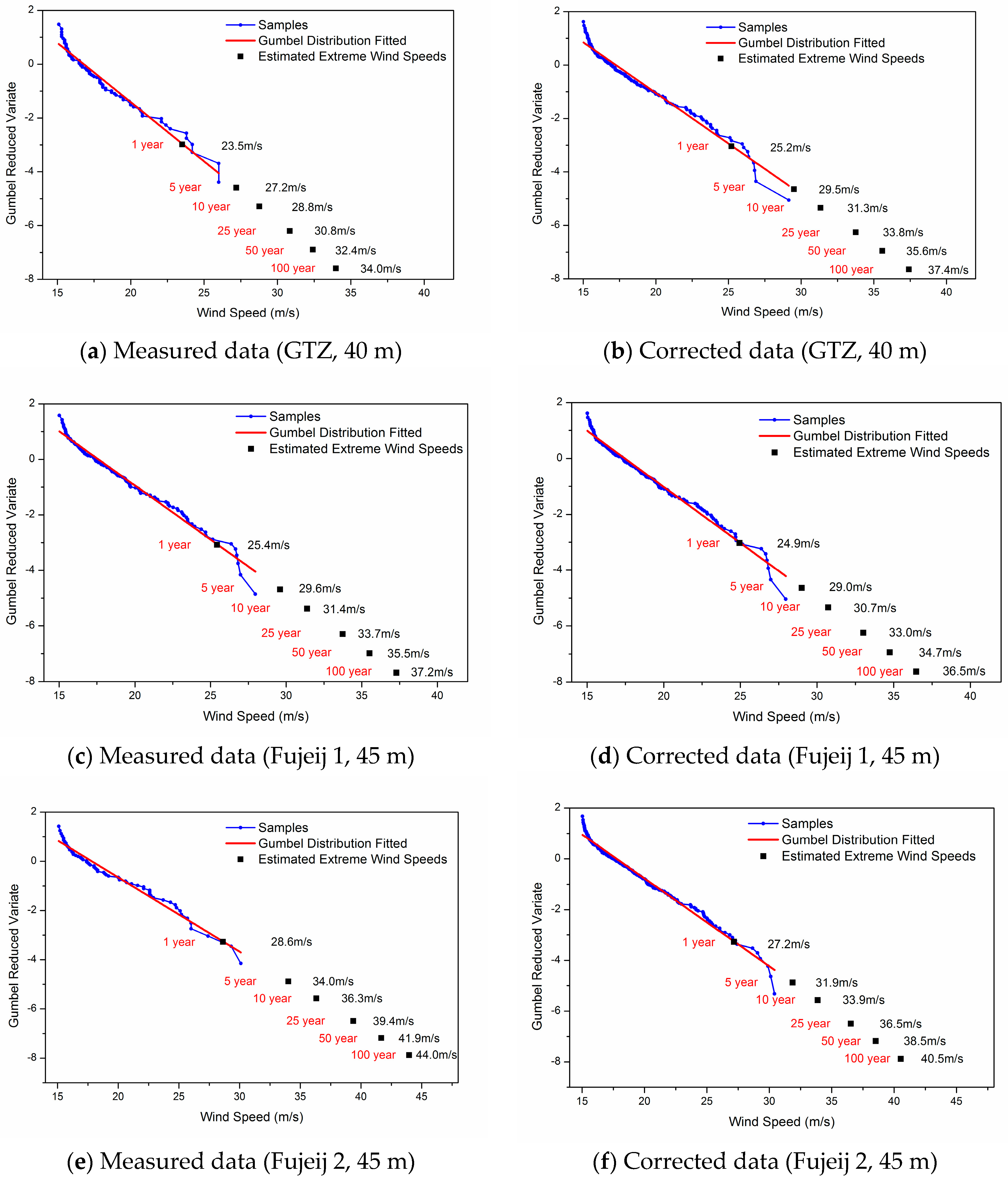
2.2. Extreme Wind Speed

EWS is an important metric in the evaluation of site compliance from the design perspective of a wind turbine. IEC 61,400 suggests that load analyses of wind turbines must be conducted with a recurrence period of 50 years under extreme wind conditions. EWS is the highest wind speed statistically expected over a long period. Many turbines that are equipped with long blades have been developed, owing to technological advances in the design and manufacturing of blades. A large blade span intensifies the aerodynamic load on a blade, increasing the vulnerability of the blade and the wind turbine to fatigue and extreme loads. Therefore, it becomes more significant to predict the EWS to ensure the integrity of the wind turbine during the period of operation.

The Gumbel distribution was used to estimate the extreme distribution of each return period because it has produced the most accurate results in previous studies [43]. The Gumbel distribution $F\left(x\right)$ is a cumulative distribution with parameters $\alpha$ and $\beta$, given by:

$$F\left(x\right)=\exp \left[-{\exp }^{-\alpha \left(v_e-\beta \right)}\right],$$

(9)

where $v_e$ is a sample corresponding to the maximum value of wind speed and $\alpha$ and $\beta$ denote the measure of dispersion (or scale parameter) and the mode of extreme value distribution (or the location parameter), respectively [34,44].

Assuming that it follows the Gumbel distribution, the EWS $V\left(p\right)$ with a return period $p$ is calculated using:

$$V\left(p\right)=-\frac{1}{\alpha }\ln \left[\ln \left(\frac{\lambda p}{\lambda p-1}\right)\right]+\mathsf{\beta },$$

(10)

where $\lambda$ denotes the extracted extreme events per year [44]. The Gumbel distribution can be employed to determine the parameters corresponding to the most suitable distribution types for the extracted samples, and the parameters were estimated using the least squares method. To estimate the Gumbel distribution, the Weibull (or probability) plotting position was used as follows:

$$WP=\frac{j}{N+1},$$

(11)

where $j$ is an integer denoting the samples sorted in ascending order and $N$ denotes the total number of samples. Thus, $WP$ is the mean value of the jth order statistic in a sample set of size $N$. Note that this is an unbiased, non-parametric estimate because no assumption involving the distribution type is entailed [45]. In addition, the Gumbel distribution graph is illustrated using Gumbel reduced variates, GG, as follows:

$$\mathrm{GG}=\ln \left(-\ln WP\right).$$

(12)

2.3. Mutually Complementary Measure-Correlate-Predict Method

The mutually complementary MCP method is a simple yet effective approach. The main advantage of the proposed approach is that it can recreate long-term data using several short-term datasets that are highly correlated; this is because each short-term dataset serves as a reference for the others. In contrast, other MCP methods require long-term reference data. Therefore, if several highly correlated short-term datasets are available, but the data corresponding to many periods are missing, the proposed approach can effectively reconstruct a long-term time-series wind dataset. More specifically, the proposed method can only be applied to short datasets that have overlapping periods and are highly correlated. The detailed procedure is presented in Figure 1, and the process is explained subsequently.

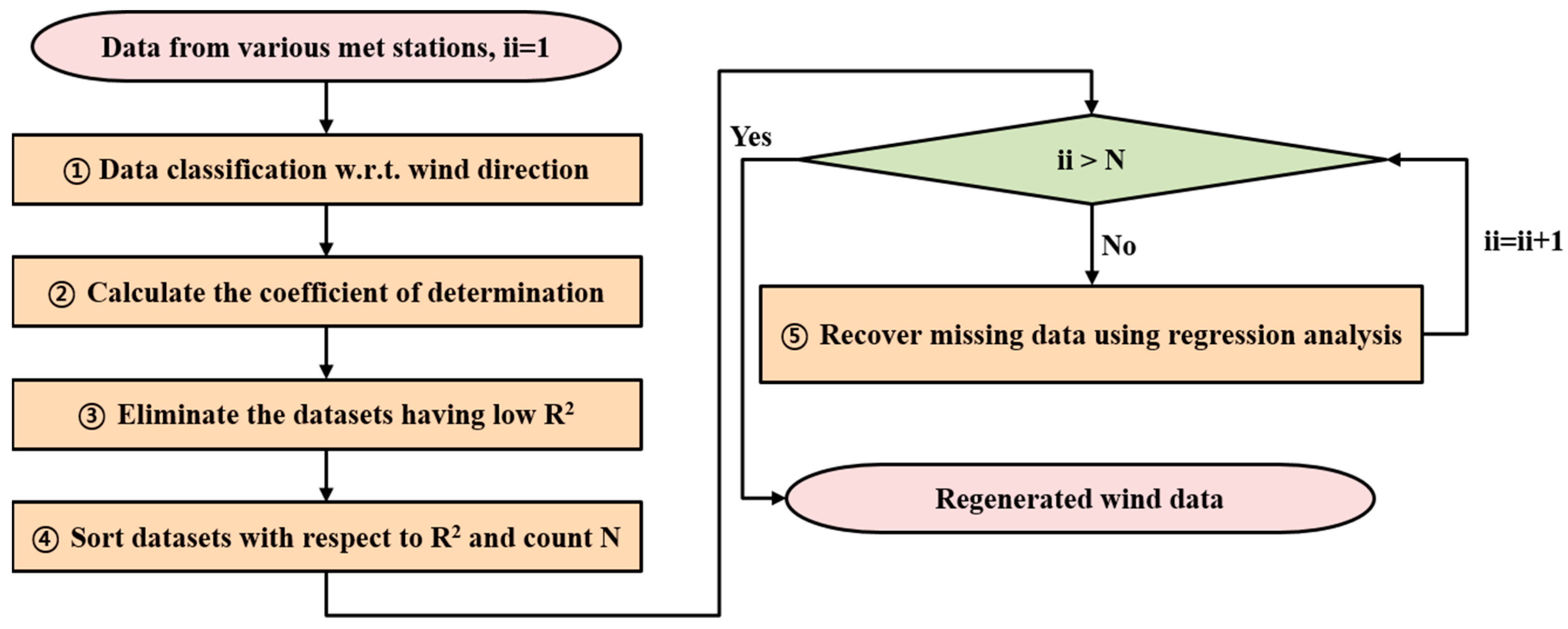
• In step, categorize all the datasets collected at a wind farm and near a site with regards to each wind direction. The number of direction sectors depends on the site characteristics. Optimum numbers can be decided by observing the wind rose of a site. In general, 12 sectors are used.
• In step ②, use the categorized data to calculate the coefficient of determination $R^2$ between datasets using Equation (13). Note that using many measured sample datasets enhances the accuracy and reliability of the mutually complementary MCP method in analyzing wind resources, similar to any other MCP method.

  $$R^2={\left(\frac{n\left({{\displaystyle \sum }}_{i=1}^n{x}_i{y}_i\right)-\left({{\displaystyle \sum }}_{i=1}^n{x}_i\right)\left({{\displaystyle \sum }}_{i=1}^n{y}_i\right)}{\sqrt{n\left({{\displaystyle \sum }}_{i=1}^n{x}_i^2\right)-{\left({{\displaystyle \sum }}_{i=1}^n{x}_i\right)}^2}\sqrt{n\left({{\displaystyle \sum }}_{i=1}^n{y}_i^2\right)-{\left({{\displaystyle \sum }}_{i=1}^n{y}_i\right)}^2}}\right)}^2,$$

  (13)

  where $x_i$ and $y_i$ denote the measured data from each met-mast.
• Once correlations among all the datasets are calculated, the sections with very poor correlations between datasets are selected and removed in step ③, because data that are poorly correlated have lower reliability for the prediction of long-term wind potentials. Generally, datasets showing R² > 0.8 are recommended to ensure accuracy and reliability in an MCP process [46].
• In step ④, sort sections in descending order of correlations and count the number of datasets.
• Use the dataset with the highest correlation to recreate the data of a recoverable period by primarily using a regression analysis in step ⑤. Then, use the datasets with the highest correlations to recreate the data of the recoverable periods. Note that the data obtained at each met-mast become a reference for those obtained at other met-masts.
• Finally, the long-term wind data from all met-masts are serially ordered and recreated in a mutually complementary manner.

3. Evaluation and Characterization of Wind Resources

Long-term wind resources of the site of interest, where seasonal and year-on-year variations are significant, were evaluated in this study. Analysis of the site requires an alternative method to assess long-term wind potentials, because long-term reference data are not available for the area under consideration and some long-term measurement datasets have several missing periods. In Section 3.1, information on the site and its data are provided. The availability of the data measured from the three met-masts was also analyzed. In Section 3.2, long-term wind potentials are characterized for Fujeij. The analysis clearly shows the effects of seasonal and year-on-year variations on the assessments of long-term wind resources.

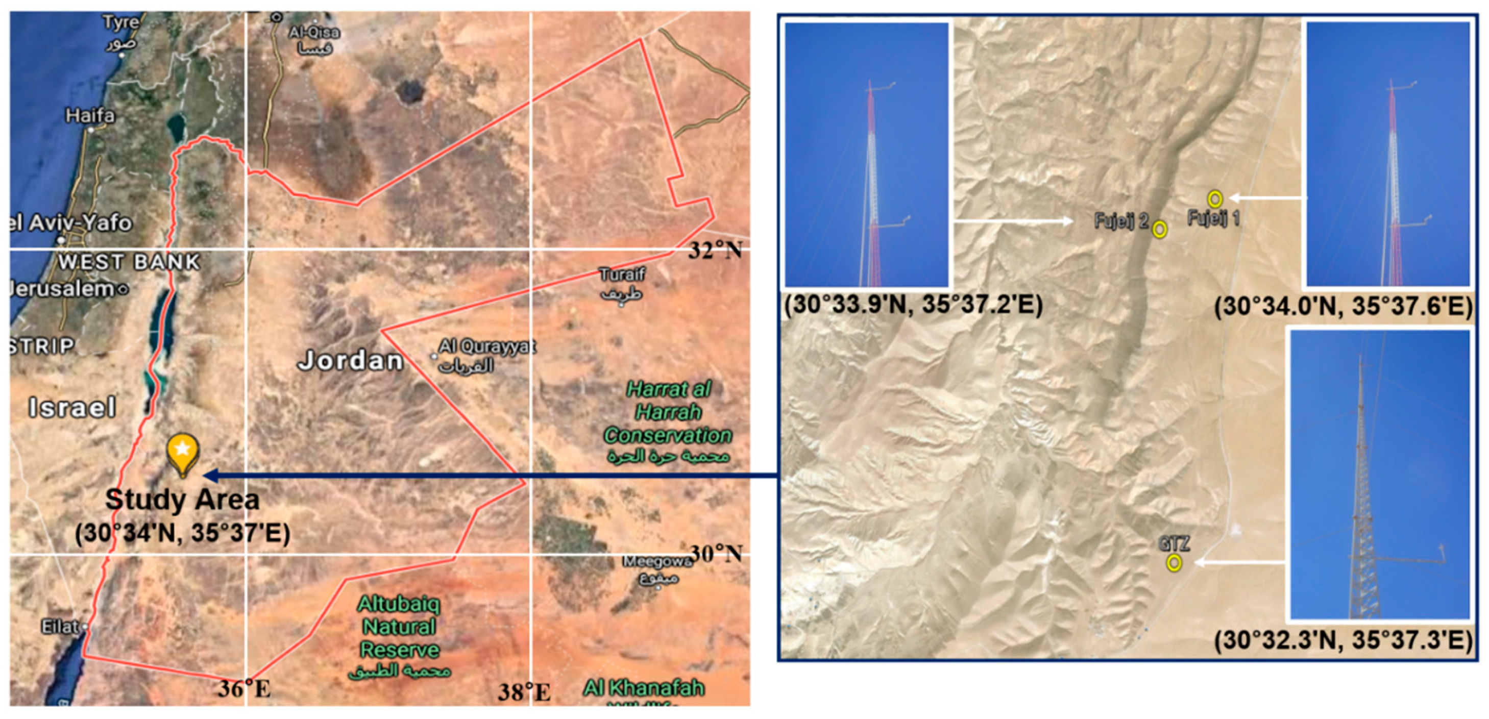
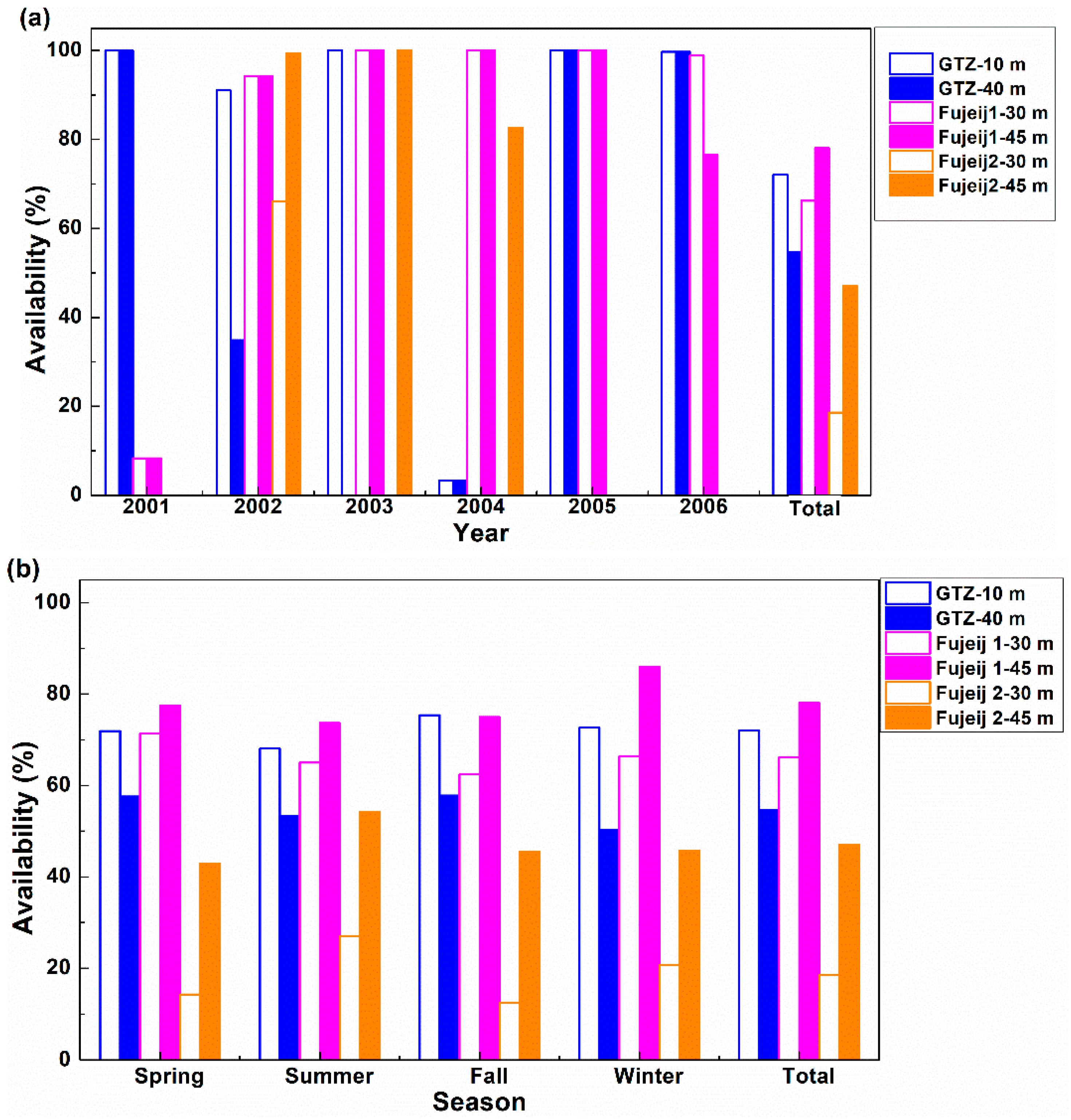
3.1. Site and Data Description

The geographical locations of the met-masts are shown in Figure 2. Six datasets gathered from three met-masts were used in this study. The area under consideration is located at the intersection of latitude 30°35′ N and longitude 35°37′ E. This area lies on top of a plateau at an elevation of approximately 1250 m. The area is predominantly a desert. Hence, the ground is mostly covered by bare rocks and scattered shrubs.

To evaluate the economic feasibility of constructing a commercial wind farm, meteorological data were measured at three met-masts, named GTZ, Fujeij 1, and Fujeij 2, which were installed in 2000, 2001, and 2002, respectively. All the met-masts were designed and installed according to IEC standards [47].

GTZ has a lattice structure and is equipped with two anemometers, one wind vane, two temperature sensors, and one air pressure sensor. One anemometer was mounted on top of the mast at a height of 40 m. The other anemometer was boom-mounted at 10 m. A wind vane was boom-mounted at 38 m. The boom-mounted anemometer and wind vane were oriented toward the west, the main wind direction at the site. The temperature sensors were mounted at heights of 38 m and 3 m, respectively. The air pressure sensor was located inside a data logger cabinet. The measured temperature $T$ and air pressure $B$ were used to calculate the air density ${\rho }_a$ of the area under consideration using Equation (6).

Both Fujeij 1 and Fujeij 2 are equipped with two prop-vanes, which measure wind speed and direction. One prop-vane was mounted on top of the mast at 45 m, whereas the other was boom-mounted at 30 m, and both were oriented toward the east. Data loggers were programmed to record the mean wind speed, standard deviation of wind speed, and wind direction, as well as the maximum and the minimum wind speeds at ten-minute intervals. More details are presented in

Table 1. Specific information of met-masts.

Name	Latitude	Longitude	Measurement Period	Mean Interval	Measurement Heights
GTZ	N 30°32.293′	E 35°37.347′	August 2000–February 2008	10 min	10 m and 40 m
Fujeij 1	N 30°34.049′	E 35°’37.615′	December 2001–February 2008	10 min	30 m and 45 m
Fujeij 2	N 30°33.991′	E 35°’37.250′	June 2002–December 2006	10 min	30 m and 45 m

.

The three met-masts are close to each other. The distance between GTZ and Fujeij 1 is approximately 3.5 km and that between Fujeij 1 and Fujeij 2 is approximately 0.6 km. Moreover, there is no obstacle or significant change in the elevation among the met-masts, as shown in Figure 2, suggesting that the wind characteristics of the three met-masts would be highly correlated. The total periods of measurement were 90, 75, and 55 months for GTZ, Fujeij 1, and Fujeij 2, respectively. Based on these, the period of interest was set to 72 months (2001–2007) because a recent study showed that the wind potential estimated after six years of measurement is similar to that derived via predictions corresponding to over 20 years [48]. More specifically, a six-year wind potential span can represent that of 20 years. Even though the data were recorded over a long period, the availability of data was poor because of the improper operation and maintenance of the three met-masts. The sensors on the met-masts were not maintained or repaired in a timely manner, leading to many periods with missing data. Hence, the measured data were cleaned after first analyzing the log files. This process eliminated abnormal data obtained during periods of malfunction, icing, and so on.

The detailed availability of the six datasets was ensured after data cleaning, as shown in Figure 3. The meteorological data measured at GTZ exhibited availabilities of 71.5% and 53.9%, at the heights of 10 and 40 m, respectively, for the period of interest. The data measured for Fujeij 1 at heights of 30 and 45 m showed availabilities of 66.2% and 78.1%, respectively, whereas those for Fujeij 2 exhibited 18.6% and 47.1%, respectively. These poor dataset availabilities imply that it is difficult to accurately predict wind potentials for the site of interest.

Figure 3a shows the annual availability of meteorological data obtained from the three met-masts. Data availability is very low for GTZ in 2004 and Fujeij 1 in 2001. In addition, the data availability for Fujeij 2 is almost zero for three years, namely, 2001, 2005, and 2006. This observation suggests that year-on-year variations cannot be correctly estimated with the measured data. Note that annual missing data also significantly affect the accuracy of the EWS estimation. Moreover, the seasonal availability of most of the datasets is less than 70% (Figure 3b), suggesting that seasonal variations can affect the prediction of wind characteristics. Hence, it is difficult to predict long-term wind resources accurately with these measurements, suggesting that the data should be corrected using an MCP method to ensure the reliability and accuracy of assessments. Interestingly, it can be observed that the data availability for GTZ at 40 m decreases every year from 2001 to 2004, and then increases in 2005. This observation can be explained based on the repairing of the anemometer at the height of 40 m in August 2004. Following this, it could measure the wind speed accurately. Thus, operational maintenance is important for the reliable measurement of long-term wind data.

Depending on the availability of meteorological data, long-term reference data are necessary to assure the prediction of long-term wind potential. Hence, several units of the available long-term reference data were analyzed. First, long-term datasets measured from meteorological stations located nearby were correlated to the short-term data measured at the site of interest. Second, reanalysis datasets from NCAR–NCEP/MERRA were correlated to the short-term data measured at the site. However, the long-term reference datasets mentioned earlier have a low correlation with the short-term measurements. Specifically, the coefficient of determination $R^2$ for the long-term datasets obtained from meteorological stations is less than 0.2, and those for the nearest reanalysis data of NCAR–NCEP and MERRA at 50 m and wind datasets from Fujeij 1 at 45 m are 0.671 and 0.341, suggesting that these datasets are not suitable as long-term references. Note that the long-term wind potential data obtained from meteorological stations were generally measured at a height of 10 m from the ground. Consequently, this produces a very low correlation because uneven terrain strongly affects wind speed at this height. Hence, for most cases, these data are not suitable as a long-term reference dataset. The reanalysis datasets of NCAR–NCEP and MERRA frequently show a low correlation because of the sparse spatial resolution. This is one of the reasons for the construction of a metrological mast with a height of over 50 m at the wind farm candidate site to assess economic feasibility.

To overcome the aforementioned non-availability of appropriate long-term data, the mutually complementary MCP method was employed to process the short-term data. This method recreates missing and unmeasured periods in the datasets of all met-masts in a mutually complementary manner. When the mutually complementary MCP method was employed, the datasets of the three met-masts were reconstructed with an availability of 99% for all datasets. The coefficient of determination, $R^2$, between the datasets is in the range of 0.8–0.99. Moreover, $R^2$ for the main wind directions is above 0.96, suggesting that the data from the three met-masts are highly correlated. Note that correlation is one of the most important factors in assuring the accuracy and reliability of long-term wind potential when applying MCP methods. Long-term wind data corrected with reference data with a low correlation are ineffective in the assessment of wind potentials. Nevertheless, reliable assessments with recovered long-term datasets are possible. Note that such recovery is possible in the case where datasets have a sufficient number of overlapping periods and are highly correlated to each other, suggesting that these assumptions require careful consideration when this method is applied.

In summary, the periods of available measurements for GTZ, Fujeij 1, and Fujeij 2, were approximately two years, six years, and four years, respectively. Nevertheless, the wind potentials for the three met-masts can be analyzed for the long term, using datasets corresponding to six years after the application of the mutually complementary MCP method.

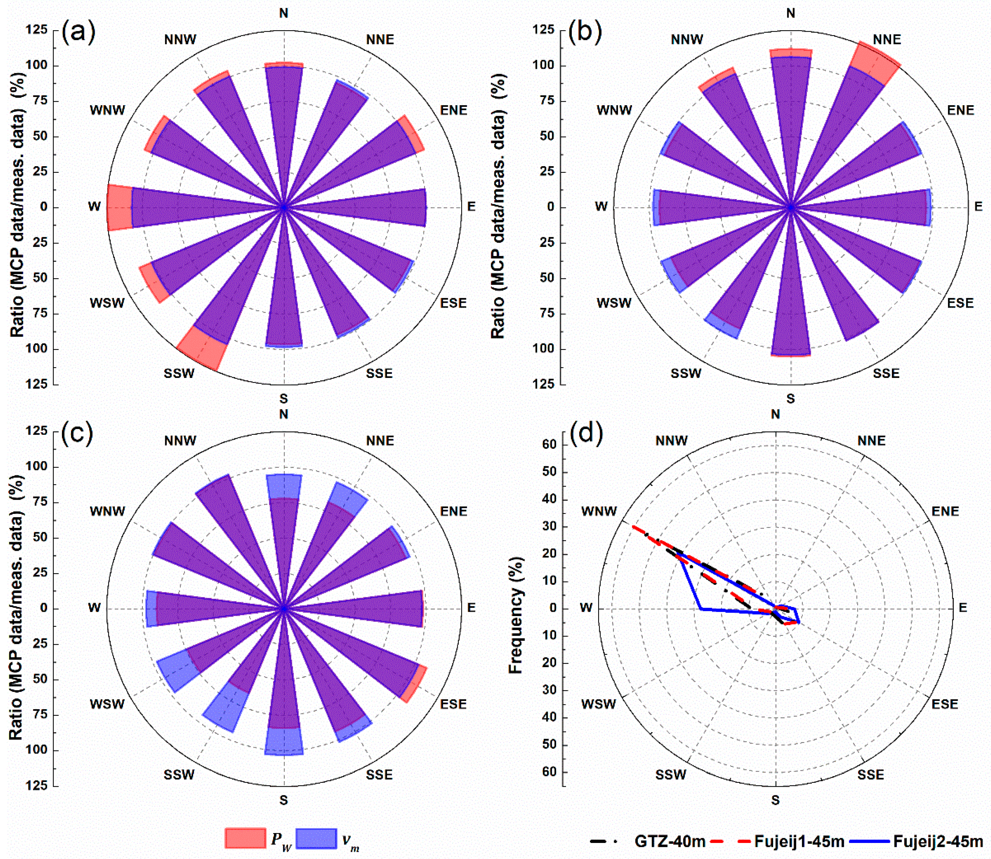
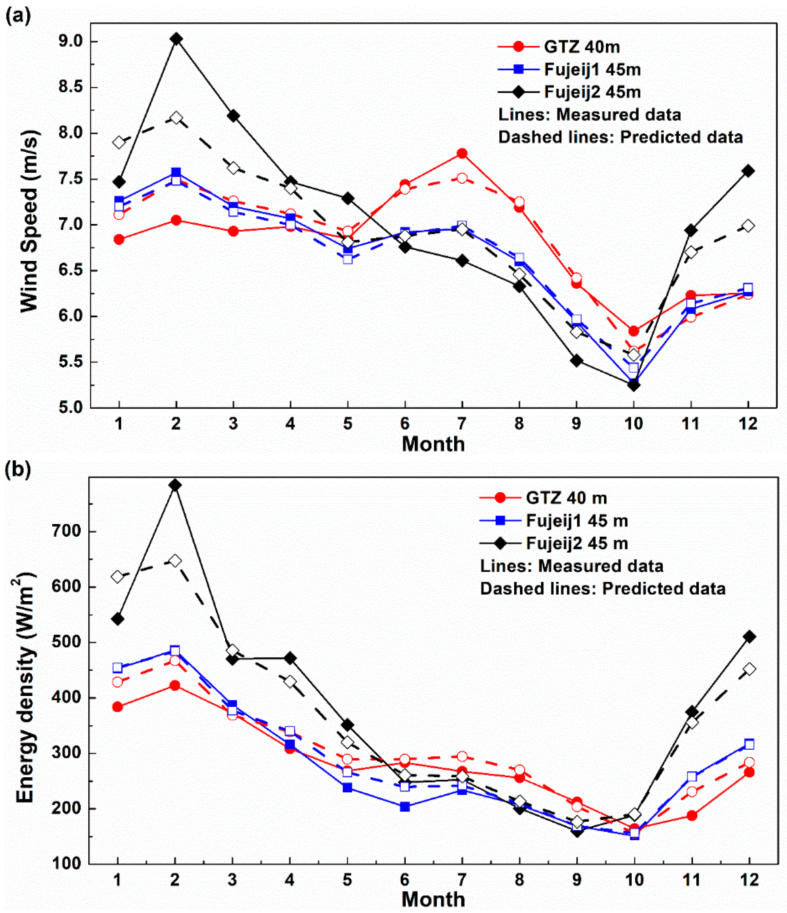
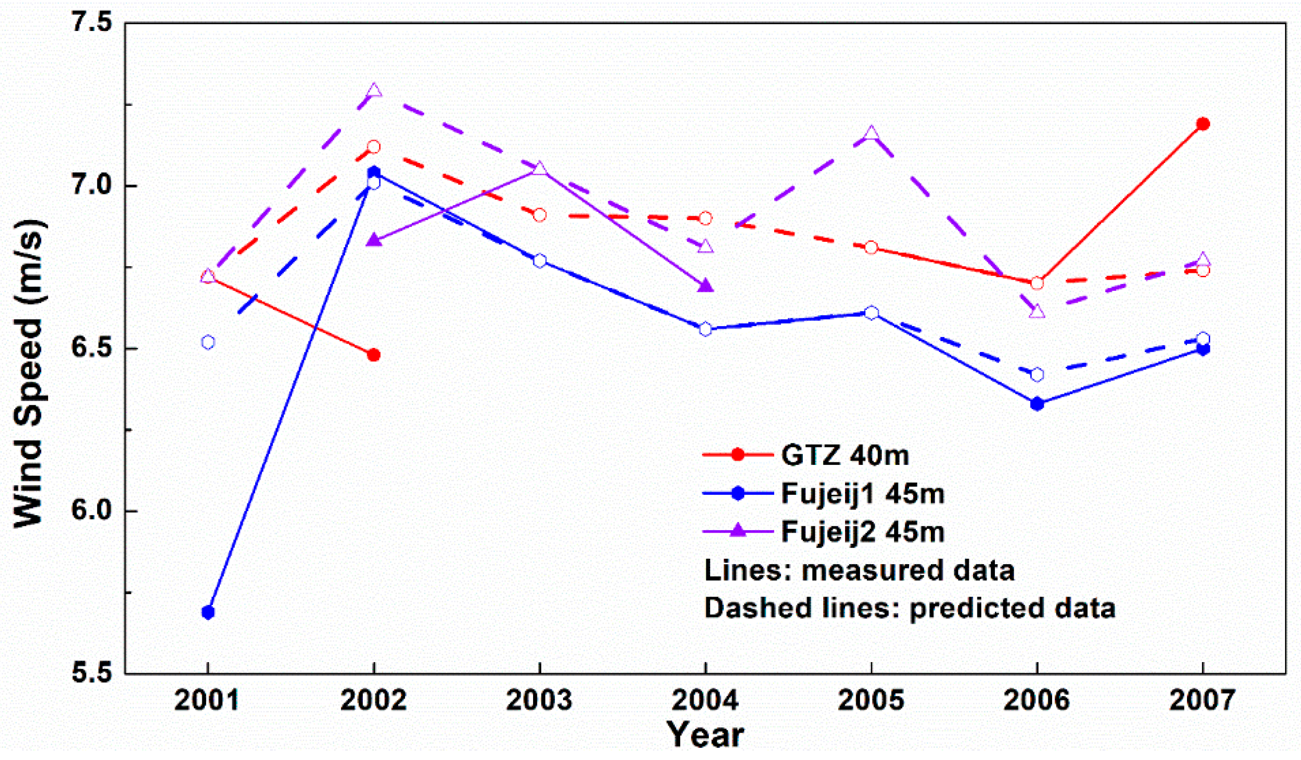
3.2. Long-Term Wind Characteristics

To accurately assess the wind potential of an area, the air density ${\rho }_a$ should be calculated first. The energy density $P_W$ and $\mathrm{AEP}$ are linearly proportional to the air density ${\rho }_a$ of a site. The monthly mean air density was calculated with the air pressure $B$ and absolute air temperature $T$, which were measured from GTZ (Figure 4). The trends in the estimated air density ${\rho }_a$ and air temperature $T$ for three years (2001 to 2003) are shown in Figure 4. Note that $B$ and $T$ were not obtained in 2004. Moreover, the air pressure $B$ measured for the period between 2005 and 2006 exhibits significant fluctuations, even though there is no particular fault record of this in the log file. Specifically, the standard deviation for monthly air pressure is approximately 30 hPa for the period between 2005 and 2006, while it is approximately 1–5 hPa for the period between 2001 and 2003. These fluctuations may have been caused by the sensor being damaged or partially clogged, which are the most common causes. However, the precise reason for the fluctuations could not be identified because GTZ was already dismantled. Hence, the air density ${\rho }_a$ for a period of three years was used to characterize variations in the air density ${\rho }_a$ of the area under consideration.

The mean air density calculated for three years is 1.056 kg·m⁻³. This estimated value is much smaller than the standard air density of 1.225 kg·m⁻³ at mean sea level, because the area under consideration is located on a plateau at an elevation of approximately 1250 m. Moreover, the air density ${\rho }_a$ significantly depends on the season because $T$ varies seasonally, as shown in Figure 4. The difference between the maximum monthly mean air density and the minimum monthly mean air density is 8.5%. The monthly wind speeds also show a trend similar to that of the air density, suggesting that the energy density $P_W$ reflects a seasonal variation that would differ from that calculated with the annual mean air density, scale factor $c$, and shape factor $k$.

The characteristics of wind resources determined with the measured data were compared to those obtained with the predicted data using the mutually complementary MCP method (

Table 2. Characteristics of wind resources from the measured and the predicted data.

		GTZ		Fujeij 1		Fujeij 2
		10 m	40 m	30 m	45 m	30 m	45 m
Scale factor ($c$)	Measured data	6.76	7.62	7.28	7.51	7.66	7.85
	Predicted data	6.80	7.71	7.24	7.49	7.74	7.91
	Difference (%)	−0.59	−1.17	0.55	0.27	−1.03	−0.76
Shape factor ($k$)	Measured data	2.25	2.29	1.99	2.00	1.81	1.86
	Predicted data	2.16	2.20	2.05	2.05	1.88	1.94
	Difference (%)	4.17	4.09	−2.93	−2.44	−3.72	−4.12
$v_m$ [m/s]	Measured data	5.99	6.75	6.40	6.60	6.70	6.90
	Predicted data	6.02	6.83	6.41	6.63	6.80	6.92
	Difference (%)	−0.58	−0.02	−0.16	−0.45	−1.47	−0.29
$P_W$ [W/m2]	Measured data	194.6	273.1	269.9	296.6	352.2	370.7
	Predicted data	205.4	295.2	258.3	286.3	347.8	359.5
	Difference (%)	−5.53	−8.08	5.31	4.47	1.24	3.01

). Interestingly, the mean wind speed $v_m$ and scale factor $c$ estimated from the measured data are similar to those determined from the predicted data obtained with the mutually complementary MCP method. The differences among these parameters are less than 1%. However, the shape factors, $k$, estimated from the measured data differ by up to 4% from the predicted data. Moreover, these differences result in significant variations in $P_W$, namely, up to approximately 8%. This is because the mean energy density $P_W$ is nonlinearly proportional to wind speed and is therefore affected by the shape factor $k$, which determines the distribution of the wind speed.

This observation is more clearly shown in Figure 5. Particularly, Figure 5a–c show the ratios of the mean wind speed $v_m$ and mean energy density $P_W$ between the measured and predicted data for the three met-masts, respectively, for the primary wind directions. Similar to the mean wind speed $v_m$ that was estimated for the entire period, shown in Table 2, the ratio of the mean wind speed $v_m$ between the measured and predicted data over the primary wind directions is almost uniform. However, the ratio of the mean energy density $P_W$ shows significant differences in some directions because of differences in the estimation of the shape factor $k$. For example, a difference of 7% in $k$ leads to a ratio of 24% for $P_W$ when the wind is directed toward the west of GTZ, as shown in Figure 5a. Note that these large differences in $P_W$ in several directions were lessened while calculating the overall $P_W$, because $P_W$ did not show a significant difference in the main wind direction (Figure 5d) [48].

A variation in the monthly mean wind speed $v_m$ clearly demonstrates that the large difference in the shape factor $k$ between the measurements and predictions was caused by seasonal variations in wind resources. As seen in Figure 6a, the wind speed of the candidate site significantly depends on the season. Furthermore, $v_m$ is higher in winter and lower in summer. The largest difference between the maximum and minimum $v_m$ values was 46% for Fujeij 2, again suggesting that the seasonal variation would create a wide distribution in wind speed. The many missing periods depicted in Figure 3b distort the influence of seasonal wind variations. For example, the monthly mean wind speed $v_m$ for January, February, and March for Fujeij 2 was established using measured data for a period of only two years (2003 and 2004). Conversely, six-year winter data were included in the datasets from GTZ and Fujeij 1 that were used to predict wind resources with the mutually complementary MCP method. Hence, $v_m$ at the height of 45 m for Fujeij 2 shows a significant difference between the measured and predicted data (black line with diamond marks and black dashed line with diamond marks in Figure 6a). It also exhibits a significant difference when calculating the shape factor $k$ because $k$ depends on the distribution of $v_m$. Seasonal variation is also important from the design perspective because large wind speed fluctuations accelerate fatigue, thereby reducing the lifespan of wind turbines.

Seasonal variations of wind resources are more clearly characterized by the monthly mean energy density $P_W$ (Figure 6b), even though the monthly $P_W$ follows a trend similar to that of the monthly mean wind speed $v_m$. Note that the monthly mean energy density $P_W$ reflects the monthly mean air density ${\rho }_a$, which enhances the prediction accuracy. The largest differences between the maximum and minimum monthly mean energy density values were 300%, 309%, and 366% for the predicted data corresponding to GTZ, Fujeij 1, and Fujeij 2, respectively. At the target site, an extensive variation in wind speed results in energy production being four times higher in winter than in summer. This information is also useful to schedule operation and maintenance work at wind farms. Performing scheduled maintenance during summer rather than winter reduces electricity production losses and thereby maximizes the efficiency of wind farms.

The effects of the air density on the ratio of the mean energy density $P_W$ were quantitatively analyzed (Figure 7). The first bar, colored yellow, shows the result of using the simplest method to calculate $P_W$. This bar was established using the measured data and the annual mean air density, which is hereafter referred to as the reference energy density. Next, other approaches were compared with the reference energy density approach. The bar with red diagonal lines represents the energy density calculated using the measured wind data and monthly mean air density. The bar with blue leftward diagonals represents the energy density calculated with corrected wind data obtained using the proposed method and annual mean air density. Finally, the bar with purple horizontal lines represents the energy density calculated using the corrected wind data and monthly mean air density. The maximum difference is approximately 10% between the energy density calculated using measured data and annual mean air density and that calculated using corrected wind data and monthly mean air density; this also suggests that seasonal variations significantly affect the predictions of wind resources. Hence, wind resources should be carefully characterized for a site affected by seasonal variations.

The annual mean wind speed $v_m$ also changes significantly over a year (Figure 8). Note that the data obtained in 2001 from Fujeij 1 at the height of 45 m exhibit a large deviation because the data actually measured in 2001 contributed only 8.3% to the yearly mean wind speed; furthermore, these measured data cannot represent the data for the entire year. Excluding the data obtained in 2001 for Fujeij 1 at 45 m, the year-on-year variation, which is calculated by dividing the standard deviation of the annual mean wind speed by the annual mean wind speed, ranges from 2.46% to 4%, depending on data from the met-masts. Moreover, the difference between the minimum and maximum mean wind speeds ranges from 6.3% to 10.9%, depending on data from the met-masts. This observation suggests that the analysis of data from the entire period should be performed by applying the mutually complementary MCP method to reflect all factors in detail, including seasonal variations, year-on-year variations, etc., and correctly calculate important parameters including the air density ${\rho }_a$, the scale factor $c$, and the shape factor $k$.

4. Assessment of Site Compliances and Energy Production

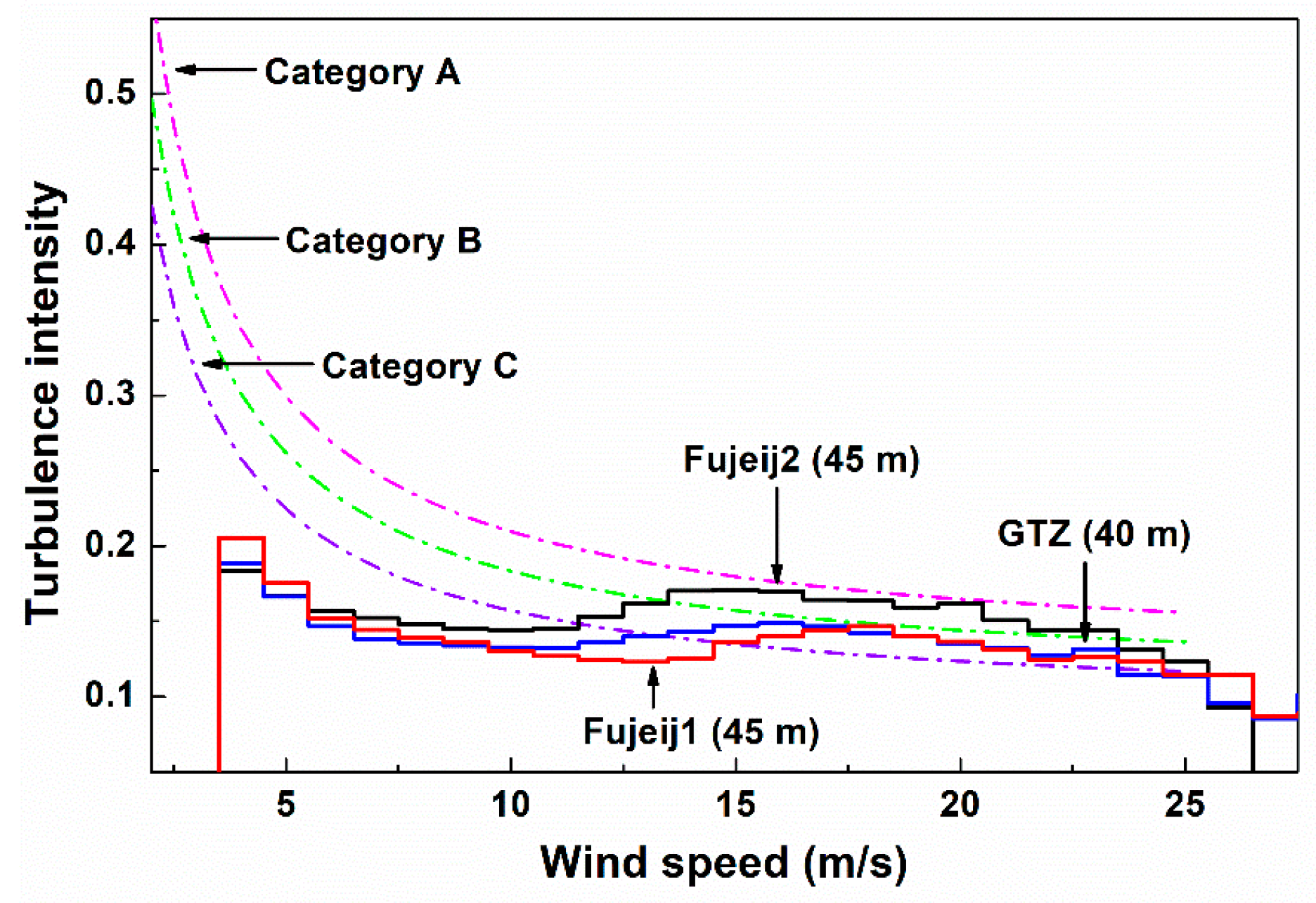
4.1. Site Compliances

The IEC categorizes wind turbines into different classes based on the EWS and turbulence intensity [10,11]. These factors are classified into three categories. For EWS, the categories are I, II, and III, while for turbulence intensity, the categories are A, B, and C under IEC 61400-1 (

Table 3. Wind turbine class [10].

Wind Turbine Class	I	II	III	S
$V_{\mathrm{ref}}$ (m/s)	50	42.5	37.5	Values specified by the designer
A $I_{\mathrm{ref}}$	0.16
B $I_{\mathrm{ref}}$	0.14
C $I_{\mathrm{ref}}$	0.12

).

The reference EWS $V_{\mathrm{ref}}$ at each class is specified in IEC 61400-1. $V_{50}$ is the extreme 10-min mean wind speed with a recurrence period of 50 years at the height of a turbine hub. Manufacturers should design wind turbines such that they can endure aerodynamic loads corresponding to the reference EWS with a recurrence period of 50 years $V_{50}.$ Therefore, a wind turbine certified as Class I should withstand a high EWS of 50 m/s, whereas a wind turbine certified as Class III should withstand a low EWS of 37.5 m/s, as depicted in Table 3. This IEC standard for certification is very important when designing a blade. As the blade length increases, the area swept by the blade to capture wind energy will also increase, thus enhancing the AEP and $\mathrm{CF}$; however, a large blade span intensifies the aerodynamic loads on the blades, rendering the blades and the wind turbine more vulnerable to material fatigue and extreme loads. Hence, the determination of the appropriate wind turbine class for a candidate site is as important as predicting long-term wind resources because diverse turbines with different blade lengths have been developed and are commercially available.

The turbulence intensities I at the three met-mast locations were characterized and are shown in Figure 9 with the IEC standards. The turbulence intensities I values at the three locations were high even though the area under consideration is mostly covered by bare rocks and scattered shrubs. The turbulence intensity for Fujeij 2 complies with category A, and those for GTZ and Fujeij 1 conform to category B. This observation is explained based on a steep cliff located to the west-northwest of the site. This cliff creates upwind flow that increases the turbulence intensity in the area under consideration. Hence, a wind turbine certified as category A is appropriate for the area under consideration. This analysis was conducted with data recorded at the top of each mast. The turbulence intensity at the hub height of an MW-class wind turbine is approximately 80 m, suggesting that the turbulence intensity at the hub height is more moderate than that indicated by the recorded data shown herein; this is because, in general, the turbulence near the ground is more intense. Obstacles and the unevenness of terrain can intensify the turbulence near the ground.

Table 4. Predicted EWS and corresponding wind turbine class for the area under consideration.

		GTZ, 40 m		Fujeij 1, 45 m		Fujeij 2, 45 m
		40 m	80 m	45 m	80 m	45 m	80 m
$V_{50}$ [m/s]	Measured data	32.4	34.5	35.5	36.5	41.9	42.6
	Corrected data	35.6	38.0	34.7	35.7	38.5	39.2
	Difference (%)	8.99	9.21	2.31	2.24	8.31	8.16
Wind turbine class	Measured data	I, II, and III		I, II, and III		I
	Corrected data	I and II		I, II, and III		I and II
CV * [%]	Measured data	6.3		5.0		9.3
	Corrected data	4.6		4.6		4.2
	Difference (%)	36.96		8.70		121.43

* CV stands for Coefficient of Variance.

and Figure 10 illustrate the EWS estimated with the corrected data using the mutually complementary MCP method. The second row for each meteorological station in Table 4 shows the EWS estimated based on shear exponents calculated for each station at a height of 80 m using the hub height of multi-MW wind turbines [49]. Based on the EWS estimated with the data measured at GTZ and Fujeij 1, wind turbines of any class can be installed on this site. In contrast, only a wind turbine certified as Class I can be installed in the area under consideration for the EWS estimated with the data measured at Fujeij 2. These differences in the EWS results with regard to the met-masts are caused by the periods for which data were unavailable.

When the mutually complementary MCP method is applied, the estimated EWS differs by up to 9% from that estimated with short-term measured data. Interestingly, the EWS estimated for the location of Fujeij 2 decreases; therefore, Class I or II wind turbines can be used in the area under consideration. As the reconstruction of the data corresponding to the missing periods diminishes deviations and increases reliability, it is possible to speculate on the collection of mutually similar values using decreasing uncertainty and coefficient of variance. In particular, strong winds were measured at Fujeij 1 and Fujeij 2 during the periods for which data were not obtained at GTZ; the EWS surge values were determined based on these available data, but the predicted values decreased when long-term data were used. Furthermore, the strong winds were not measured at GTZ during the periods with missing data, and this can be corrected by introducing the mutually complementary MCP method. Consequently, it is possible to identify an increase in the EWS. Note that the wind turbine class is decided conservatively only when several datasets are available for the site because the reliability of the system is the most important factor when studying the feasibility of power plants.

4.2. Assessment of Energy Production

Using the estimated wind potential, the AEP and CF of wind turbines widely in use were calculated and are summarized in

Table 5. Estimation of the annual energy production (AEP) and capacity factor (CF) ($c$: 7.49, $k$: 2.05).

Manufacturer	Turbine Class	Rated Power (kW)	Rotor Diameter (m)	AEP (MWh)	AEP/MW (MWh)	CF (%)
VESTAS	IIA	3000	112	9158	3053	34.8
Alstom	IIA	3000	110	8945	2982	34.0
Gamesa	IIA	4500	128	13,312	2958	33.8
REpower	IIA	3300	104	9114	2762	31.5
Alstom	IA	3000	100	8076	2692	30.7
REpower	IB	5000	126	12,519	2504	28.6
Siemens	IA	3600	107	8990	2497	28.5
VESTAS	IA	2000	80	4896	2448	27.9
GE Wind	IB	3600	104	8757	2433	27.8
VESTAS	IIA	3000	90	6656	2219	25.3
ENERCON	IA	7500	127	16,353	2180	24.9

. The data from Fujeij 1 were used, and the estimated wind potential parameters were adjusted to the hub height using the measured wind shear exponent [23].

The EWS predicted with the measured data required that a Class I wind turbine should be selected to ensure the safety and reliability of the wind farm. In this regard, the maximum CF of the Alstom ECO100 Class I wind turbine is 30.7%, and this turbine can be employed in the target site. Meanwhile, turbines classified as Class II are included as candidates while applying the mutually complementary MCP method. The CF of Class II wind turbines is approximately 31.5–34.8%. In general, the CF of Class II wind turbines is higher than that of Class I wind turbines because of the longer blades. Considering that a wind farm operates for over 20 years, the turbine class determined based on the EWS is critical in the assessment of long-term wind resources and significantly affects economic feasibility. It is emphasized that the EWS is more critical than the mean wind speed in analyzing the economic feasibility of a wind farm, as many new wind turbines have been designed, certified as Class II or III, and launched on the market.

5. Conclusions

This study presents the mutually complementary MCP method to ensure the reliability of long-term wind resources for sites for which long-term data are unavailable. The following conclusions can be drawn based on the results of the analysis.

• The mutually complementary MCP method is simple yet effective for sites characterized by seasonal and year-on-year variations, where long-term reference data for estimating wind potentials and EWS are unavailable. The various periods of missing data corresponding to different masts result in the inconsistent determination of turbine classes based on the EWS, thereby confounding the estimation of site compliance.
• Because of extensively variable wind distributions, the energy density $P_W$ is a more sensitive metric than the mean wind speed $v_m$ for sites characterized by seasonal and year-on-year variations. Specifically, a difference of up to 4% in the shape factor $k$ results in a change of over 20% in the mean energy density $P_W$.
• Similarly, the scale factor $c$ and the shape factor $k$, which govern the energy density $P_W$ of the site, are more important than the mean wind speed $v_m$.
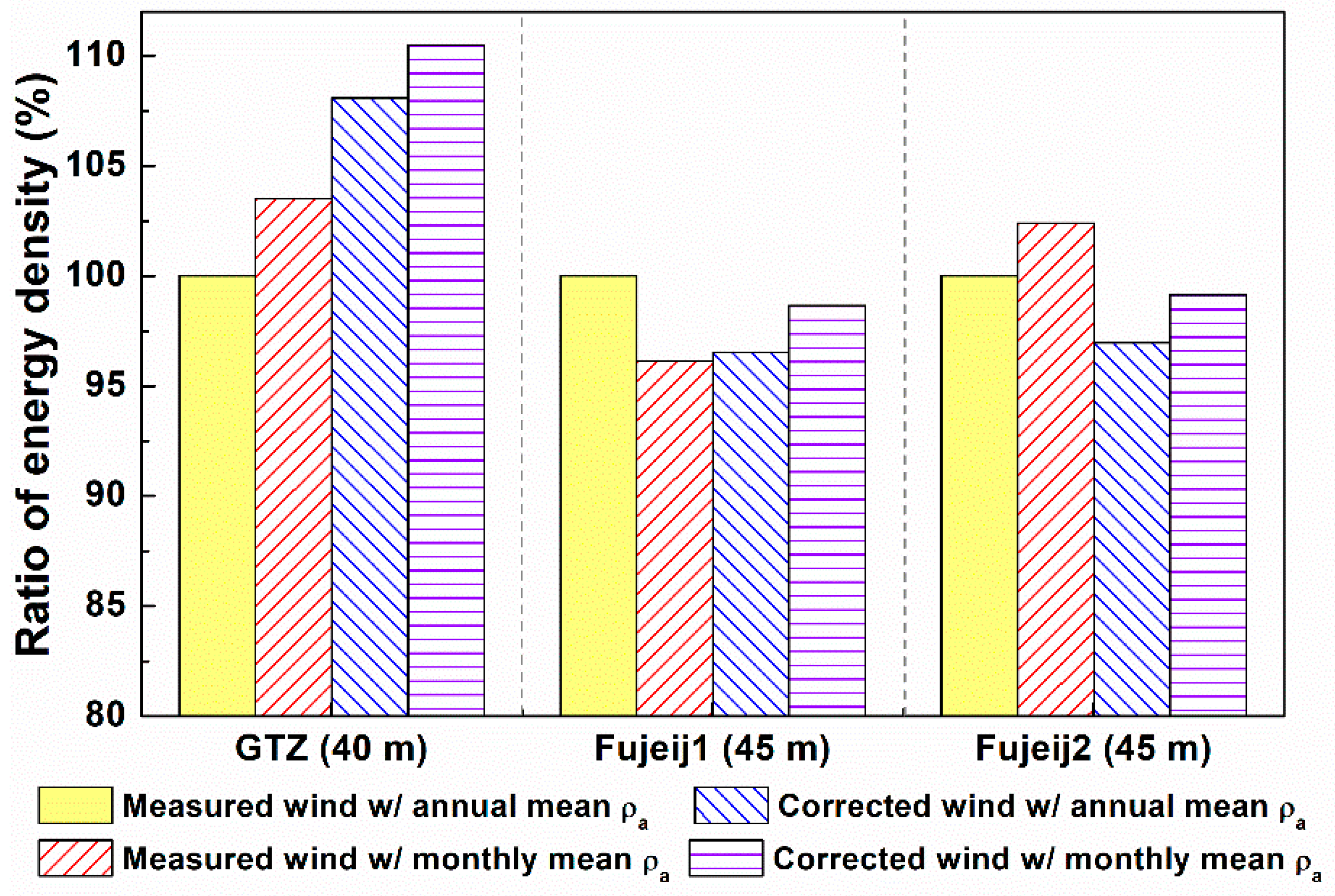
• The seasonal variation in the air density ${\rho }_a$ should be considered when calculating $P_W$, as the variations in ${\rho }_a$ cause an error in the prediction of long-term wind potential.

Note that the proposed method was validated with a single case study because large-scale wind datasets are extremely difficult to obtain and the wind datasets of most commercial wind farms are confidential. In the future, the proposed method can be validated with more wind datasets as they become available.

References

1. Twidell, J.; Weir, T. Renewable Energy Resources, 2nd ed.; Taylor Francis E-Library: Oxfordshire, UK, 2006. [Google Scholar]
2. Oh, K.-Y.; Nam, W.; Ryu, M.S.; Kim, J.-Y.; Epureanu, B.I. A review on the foundations of offshore wind energy convertors: Current Status and future perspectives. Renew. Sustain. Energy Rev. 2018, 88, 16–36. [Google Scholar] [CrossRef]
3. Dong, L. Wind resource assessment in the southern plains of the US: Characterizing large-scale atmospheric circulation with cluster analysis. Atmosphere 2018, 9, 110. [Google Scholar] [CrossRef] [Green Version]
4. Ruiz, A.; Onea, F.; Rusu, E. Study concerning the expected dynamics of the wind energy resources in the Iberian nearshore. Energies 2020, 13, 4832. [Google Scholar] [CrossRef]
5. Menezes, D.; Mendes, M.; Almeida, J.A.; Farinha, T. Wind farm and resource datasets: A comprehensive survey and overview. Energies 2020, 13, 4702. [Google Scholar] [CrossRef]
6. Barthelmie, R.J.; Shepherd, T.J.; Aird, J.A.; Pryor, S.C. Power and wind shear implications of large wind turbine scenarios in the US central plains. Energies 2020, 13, 4269. [Google Scholar] [CrossRef]
7. Young, I.R.; Kirezci, E.; Ribal, A. The global wind resource observed by scatterometer. Remote Sens. 2020, 12, 2920. [Google Scholar] [CrossRef]
8. Global Wind Statistics 2017; Global Wind Energy Council: Brussel, Belgium, 2018.
9. Hales, D. Renewables 2018 Global Status Report; IEA: Paris, France, 2018. [Google Scholar]
10. IEC 61400 Wind Turbines—Part 1: Design Requirements; IEC: Geneva, Switzerland, 2005.
11. IEC 61400 Wind Turbines—Part 3: Design Requirements for Offshore Wind Turbines; IEC: Geneva, Switzerland, 2009.
12. Thøgersen, M.L.; Sørensen, T. Measure-Correlate-Predict methods: Case studies and software implementation. In Proceedings of the EWEC-2007, Milan, Italy, 7–10 May 2007. [Google Scholar]
13. Kaldellis, J.K.; Kavadias, K.A.; Filios, A.E. A new computational algorithm for the calculation of maximum wind energy penetration in autonomous electrical generation systems. Appl. Energy 2009, 86, 1011–1023. [Google Scholar] [CrossRef]
14. Erdem, E.; Shi, J. ARMA based approaches for forecasting the tuple of wind speed and direction. Appl. Energy 2011, 88, 1405–1414. [Google Scholar] [CrossRef]
15. Velázquez, S.; Carta, J.A.; Matías, J.M. Comparison between ANNs and linear MCP algorithms in the long-term estimation of the cost per kW h produced by a wind turbine at a candidate site: A case study in the Canary Islands. Appl. Energy 2011, 88, 3869–3881. [Google Scholar] [CrossRef]
16. Liu, H.; Erdem, E.; Shi, J. Comprehensive evaluation of ARMA–GARCH(-M) approaches for modeling the mean and volatility of wind speed. Appl. Energy 2011, 88, 724–732. [Google Scholar] [CrossRef]
17. Dong, Y.; Wanga, J.; Jiang, H.; Shi, X. Intelligent optimized wind-resource assessment and wind turbines selection in Huitengxile of Inner Mongolia, China. Appl. Energy 2013, 109, 239–253. [Google Scholar] [CrossRef]
18. Carvalho, D.; Rocha, A.; Santos, C.S.; Pereira, R. Wind resource modelling in complex terrain using different mesoscale–microscale coupling techniques. Appl. Energy 2013, 108, 493–504. [Google Scholar] [CrossRef] [Green Version]
19. Rogers, A.L.; Rogers, J.W.; Manwell, J.F. Comparison of the performance of four measure-correlate-predict algorithms. J. Wind Eng. Ind. Aerodyn. 2005, 93, 243–264. [Google Scholar] [CrossRef]
20. Carta, J.A.; Velázquez, S. A new probabilistic method to estimate the long-term wind speed characteristics at a potential wind energy conversion site. Energy 2011, 36, 2674–2685. [Google Scholar] [CrossRef]
21. Guo, Z.; Zhao, J.; Zhang, W.; Wang, J. A corrected hybrid approach for wind speed prediction in Hexi Corridor of China. Energy 2011, 36, 1668–1679. [Google Scholar] [CrossRef]
22. Ali, S.; Lee, S.-M.; Jang, C.-M. Forecasting the long-term wind data via measure-correlated-predict (MCP) methods. Energies 2018, 11, 1541. [Google Scholar] [CrossRef] [Green Version]
23. Xu, C.; Hao, C.; Li, L.; Han, X.; Xue, F.; Sun, M.; Shen, W. Evaluation of the power-law wind-speed extrapolation method with atmospheric stability classification methods for flows over different terrain types. Appl. Sci. 2018, 8, 1429. [Google Scholar] [CrossRef] [Green Version]
24. Woods, J.C.; Watson, S.J. A new matrix method of predicting long-term wind roses with MCP. J. Wind Eng. Ind. Aerodyn. 1997, 66, 85–94. [Google Scholar] [CrossRef]
25. Lackner, M.A.; Rogers, A.L.; Manwell, J.F. The round robin site assessment method: A new approach to wind energy site assessment. Renew. Energy 2008, 33, 2019–2026. [Google Scholar] [CrossRef]
26. Lackner, M.A.; Rogers, A.L.; Manwell, J.F. Uncertainty analysis in mcp-based wind-resource assessment and energy production estimation. J. Sol. Energy Eng. 2008, 130, 031006-1–031006-10. [Google Scholar] [CrossRef]
27. Kim, H.-G.; Kim, K.-Y.; Kang, Y.-H. Comparative evaluation of the third-generation reanalysis data for wind resource assessment of the southwestern offshore in South Korea. Atmosphere 2018, 9, 73. [Google Scholar]
28. Shi, X.; Lei, X.; Huang, Q.; Huang, S.; Ren, K.; Hu, Y. Hourly day-ahead wind power prediction using the hybrid model of variational model decomposition and long short-term memory. Energies 2018, 11, 3227. [Google Scholar] [CrossRef] [Green Version]
29. Liu, H.; Duan, Z.; Chen, C.; Wu, H. A novel two-stage deep learning wind speed forecasting method with adaptive multiple error corrections and bivariate Dirichlet process mixture model. Energy Convers. Manag. 2019, 199, 111975. [Google Scholar] [CrossRef]
30. Jang, J.-K.; Yu, B.-M.; Ryu, K.-W.; Lee, J.-S. Offshore wind-resource assessment around Korean Peninsula by using QuikSCAT satellite data. J. Korean Soc. Aeronaut. Space Sci. 2009, 37, 1121–1130. [Google Scholar]
31. Chelton, D.B.; Freilich, M.H.; Sienkiewicz, J.M.; Ahn, J.M.V. On the use of QuikSCAT scatterometer measurements of surface winds for marine weather prediction. Mon. Weather Rev. 2006, 134, 2055–2071. [Google Scholar] [CrossRef]
32. GMAO. Global Modeling and Assimilation Office. 2014. Available online: http://gmao.gsfc.nasa.gov/merra/ (accessed on 14 August 2019).
33. Rhee, J.; Im, J. Estimating high spatial resolution air temperature for regions with limited in situ data using MODIS products. Remote Sens. 2014, 6, 7360–7378. [Google Scholar] [CrossRef] [Green Version]
34. Burton, T.; Sharpe, D.; Jenkins, N.; Bossanyi, E. Wind Energy Handbook; Wiley: Hoboken, NJ, USA, 2001. [Google Scholar]
35. Chang, T.J.; Wu, Y.-T.; Hsu, H.-Y.; Chu, C.-R.; Liao, C.-M. Assessment of wind characteristics and wind turbine characteristics in Taiwan. Renew. Energy 2003, 28, 851–871. [Google Scholar] [CrossRef]
36. Shoaib, M.; Siddiqui, I.; Amir, Y.M.; Rehman, S.U. Evaluation of wind power potential in Baburband (Pakistan) using Weibull distribution function. Renew. Sustain. Energy Rev. 2017, 70, 1343–1351. [Google Scholar] [CrossRef]
37. Seguro, J.V.; Lambert, T.W. Modern estimation of the parameters of the Weibull wind speed distribution for wind energy analysis. J. Wind Eng. Ind. Aerodyn. 2000, 85, 75–84. [Google Scholar] [CrossRef]
38. Justus, C.G.; Hargraves, W.R.; Mikhail, A.; Graber, D. Methods for estimating wind speed frequency distributions. J. Appl. Meteorol. 1978, 17, 350–353. [Google Scholar] [CrossRef]
39. Gipe, P. Wind Power: Renewable Energy for Home, Farm, and Business, 2nd ed.; Chelsea Green Publishing: Chelsea, VT, USA, 2004. [Google Scholar]
40. Dicorato, M.; Forte, G.; Pisani, M.; Trovato, M. Guidelines for assessment of investment cost for offshore wind generation. Renew. Energy 2011, 36, 2043–2051. [Google Scholar] [CrossRef]
41. Kim, J.-Y.; Oh, K.-Y.; Kang, K.-S.; Lee, J.-S. Site selection of offshore wind farms around the Korea Peninsula through economic evaluation. Renew. Energy 2013, 54, 189–195. [Google Scholar] [CrossRef]
42. Oh, K.-Y.; Kim, J.-Y.; Lee, J.-S.; Ryu, K.-W. Wind-resource assessment around Korean Peninsula for feasibility study on 100MW class offshore wind farm. Renew. Energy 2012, 42, 217–226. [Google Scholar] [CrossRef]
43. Kotz, S.; Nadarajah, S. Extreme Value Distributions: Theory and Applications; Imperial College Press: London, UK, 2000. [Google Scholar]
44. Palutikof, J.P.; Brabson, B.B.; Lister, D.H.; Adcock, S.T. A review of methods to calculate extreme wind speeds. Meteorol. Appl. 1999, 6, 119–132. [Google Scholar] [CrossRef]
45. An, Y.; Pandey, M.D. A comparison of methods of extreme wind speed estimation. J. Wind Eng. Ind. Aerodyn. 2005, 93, 535–545. [Google Scholar] [CrossRef]
46. EMD. Course Book for WindPRO Training—Basic; EMD: Darmstadt, Germany, 2010. [Google Scholar]
47. Annex, G. (Ed.) IEC 61400 Wind Turbines—Part 12-1: Power Performance Measurements of Electricity Producing Wind Turbines; IEC: Geneva, Switzerland, 2005. [Google Scholar]
48. Kim, J.-Y.; Oh, K.-Y.; Kim, M.-S.; Kim, K.-Y. Evaluation and characterization of offshore wind resources with long-term met mast data corrected by wind lidar. Renew. Energy 2019, 144, 41–55. [Google Scholar] [CrossRef]
49. Oh, K.-Y.; Kim, J.-Y.; Lee, J.-K.; Ryu, M.-S.; Lee, J.-S. An assessment of wind energy potential at the demonstration offshore wind farm in Korea. Energy 2012, 46, 555–563. [Google Scholar] [CrossRef]
Figure 1. Flowchart for the mutually complementary Measure-Correlate-Predict (MCP) method.
Mathematics 08 01795 g001
Figure 2. Geographical positions of the meteorological masts (met-masts).
Mathematics 08 01795 g002
Figure 3. (a) Annual and (b) seasonal availability of metrological data measured at three met-masts.
Mathematics 08 01795 g003
Figure 4. Monthly mean air density (solid lines) and monthly mean temperature (dashed lines).
Mathematics 08 01795 g004
Figure 5. Ratios of the mean wind speed v m and the mean energy density P W between the measured data and predicted data over direction for (a) GTZ at 40 m, (b) Fujeij 1 at 45 m, and (c) Fujeij 2 at 45 m; (d) frequency rose of wind resources. Note that dark blue color represents regions where v m and P W overlap.
Mathematics 08 01795 g005
Figure 6. Variations in (a) monthly wind speed and (b) monthly energy density estimated from metrological data from three met-masts; the solid lines represent the measured data; dashed lines are the data predicted using the mutually complementary MCP method.
Mathematics 08 01795 g006
Figure 7. Ratio of energy density with respect to data measured with annual mean air density.
Mathematics 08 01795 g007
Figure 8. Annual wind speed at the meteorological masts at various heights.
Mathematics 08 01795 g008
Figure 9. Turbulence intensity over wind speed.
Mathematics 08 01795 g009
Figure 10. Estimation of extreme wind speed (EWS) using data from the three met-masts.
Mathematics 08 01795 g010