Dependence of Dynamics of a System of Two Coupled Generators with Delayed Feedback on the Sign of Coupling

Abstract

In this paper, we study the nonlocal dynamics of a system of delay differential equations with large parameters. This system simulates coupled generators with delayed feedback. Using the method of steps, we construct asymptotics of solutions. By these asymptotics, we construct a special finite-dimensional map. This map helps us to determine the structure of solutions. We study the dependence of solutions on the coupling parameter and show that the dynamics of the system is significantly different in the case of positive coupling and in the case of negative coupling.

1. Introduction

Consider equation

$$\dot{u}\left(t\right)=-\nu u\left(t\right)+\lambda F\left(u(t-T)\right),$$

(1)

where u is a scalar function, parameters $\nu$, T, and $\lambda$ are positive, $F\left(u\right)$ is some nonlinear compactly supported function. This equation is a mathematical model in problems of radiophysics and biology. It simulates a generator with nonlinear delayed feedback with a first-order RC low-pass filter (see, for example, [1,2,3]). Such generators are used in the manufacture of sonars, noise radars, and D-amplifiers [2]. Equation (1) models a biological process where the single state variable u decays with a rate $\nu$ proportional to u in the present and is produced with a rate dependent on the value of u some time in the past [4]. Such processes arise in a variety of problems in various areas in biology (see Table 1 and references in [4]). In addition, the dynamics of Equation (1) is of general scientific interest [5,6,7,8,9,10,11,12,13]. The authors find complicated periodic solutions [5,6,7] and chaos [8] in this model in the case of “step-like” nonlinearity. In Ref. [9], authors study properties of solutions and find a global attractor of model (1) with delayed positive feedback and in the paper [10] existence and stability of relaxation cycle of the multidimensional system (1) in the case of large $\lambda$ is studied. In Refs. [11,12,13], the authors study properties of solutions of normalized Equation (1) (parameters $\nu =\lambda =1$) in the case of sufficiently large T$(T\gg 1)$. They deal with equation

$$\epsilon \dot{u}\left(t\right)=-u\left(t\right)+f\left(u(t-1)\right),$$

(2)

where $\epsilon =1/T$ and study how the dynamics of this equation when $\epsilon$ is small (when T is large in (1)) is related with dynamics of this equation in the case $\epsilon =0$.

In this paper, we deal with a system of two coupled normalized ($\nu =1$) equations of the form (1)

$$\left\{\begin{array}{c}{\dot{u}}_1+u_1=\lambda F\left(u_1(t-T)\right)+\gamma (u_2-u_1),\hfill \\ {\dot{u}}_2+u_2=\lambda F\left(u_2(t-T)\right)+\gamma (u_1-u_2).\hfill \end{array}\right.$$

(3)

Here, delay time T is a positive constant, a nonlinear sufficiently smooth function $F\left(u\right)$ is compactly supported:

$$F\left(u\right)=\left\{\begin{array}{c}f\left(u\right),\left|u\right|\le p,\hfill \\ 0,\left|u\right|>p,\hfill \end{array}\right.$$

where p is some positive constant.

We assume that function $f\left(u\right)$ on the segment $u\in [-p,p]$ satisfies the conditions:

$$\begin{array}{c}f\left(p\right)=f(-p)=0;\hfill \\ f\left(u\right)\ne 0\mathrm{except} \mathrm{for}\mathrm{a} \mathrm{finite} \mathrm{number} \mathrm{of} \mathrm{points};\hfill \\ \mathrm{if}f\left(u^{*}\right)=0,\mathrm{then}{f}^{\prime }\left(u^{*}\right)\ne 0 \mathrm{or} f^{\prime \prime }\left(u^{*}\right)\ne 0.\hfill \end{array}$$

(4)

and that coefficient $\lambda$ is large enough: $\lambda \gg 1$.

This model simulates two coupled D-amplifiers or two noise-radars with a large amount of feedback. If coupling parameter $\gamma$ is asymptotically small at $\lambda \to +\infty$, then exponentially orbitally stable relaxation cycles coexist in model (3) (see [14,15]). Now, we are interested in nonlocal dynamics of this model in the case $\gamma$ is some nonzero constant and we study how the dynamic properties of the system differ in the cases of positive and negative coupling.

The paper is organized as follows. In Section 2, we introduce some set of initial conditions and integrating by steps system (3) under some non-degeneracy conditions we construct solutions with initial conditions from the chosen set. By formulas of solution, we obtain the operator of translation along the trajectories $\mathsf{\Pi }$ and map describing dynamics of this operator. Using this map, we clarify asymptotics of solutions of system (3) in the case $\gamma >0$ in Section 3 and in the case $\gamma <0$ in Section 4. In Section 5, as an example, we consider a narrower class of functions f and prove that asymptotic formulas of solution given in Section 2, Section 3 and Section 4 are valid for a wide set of initial conditions (for all initial conditions from this set, non-degeneracy conditions hold) and prove the existence of relaxation cycles in system (3). We show that the dynamics of system (3) is significantly different in the case of positive and negative coupling in Section 6 and, in Section 7, we draw conclusions.

2. Constructing the Asymptotics of Solutions

Let’s find relaxation solutions of (3) and study the dynamics of this system. For this purpose, we consider initial conditions ${(u_1\left(s\right),u_2\left(s\right))}^T\in C_{[-T,0]}\left({\mathbb{R}}^2\right)$ outside of the strip $|u_j\left(s\right)|<p$ ($s\in [-T,0]$, $j=1,2$) and construct asymptotics of all solutions of system (3) for this set of initial conditions.

Due to the choice of initial conditions on the segment $t\in [0,T]$, system (3) has the form

$$\left\{\begin{array}{c}{\dot{u}}_1+u_1=\gamma (u_2-u_1),\hfill \\ {\dot{u}}_2+u_2=\gamma (u_1-u_2).\hfill \end{array}\right.$$

(5)

Moreover, system (3) has form (5) until at least one of the components of the solution comes into the strip $|u_j|<p$. Thus, for $t\ge 0$, until at least one of the components of the solution of system (3) for the first time comes into the strip $|u_j|<p$, a solution of system (3) has form

$$\begin{array}{c}{u}_1\left(t\right)=\frac{1}{2}(u_1\left(0\right)+u_2\left(0\right))e^{-t}+\frac{1}{2}(u_1\left(0\right)-u_2\left(0\right))e^{-(1+2\gamma )t},\\ u_2\left(t\right)=\frac{1}{2}(u_1\left(0\right)+u_2\left(0\right))e^{-t}-\frac{1}{2}(u_1\left(0\right)-u_2\left(0\right))e^{-(1+2\gamma )t}.\end{array}$$

(6)

It follows from (6) that, in the case $\gamma <-\frac{1}{2}$, there exist solutions of system (3) tending to infinity, and, in the case $\gamma =-\frac{1}{2}$, there exist solutions of system (3) tending to a constant at $t\to +\infty$. We are interested in relaxation solutions, which is why we assume further that $\gamma >-\frac{1}{2}$.

If $\gamma >-\frac{1}{2}$, then at least one component of a solution eventually comes into the strip $|u_j|<p$ ($j=1$ or 2). Let $t_1\ge 0$ be the first time moment such that some component of the solution (we denote it as $u_i$) gets inside the strip $|u_i\left(t\right)|\le p$:

$$|u_1(s+t_1)|\ge p,|u_2(s+t_1)|\ge p \mathrm{f}\mathrm{o}\mathrm{r} s\in [-T,0),$$

(7)

$|u_i\left(t_1\right)|=p$ and $|u_i\left(t\right)|<p$ if $t_1<t<t_1+\delta$ (where $\delta >0$ is some constant and i equals 1 or 2). Then,

$$u_i\left(t_1\right)=kp,u_{3-i}\left(t_1\right)=xp,$$

(8)

where k denotes the sign of $u_i\left(t_1\right)$ (parameter k takes values $-1$ or 1) and x is some value such that $\left|x\right|\ge 1$. We denote the set of pairs of initial functions ${(u_1\left(s\right),u_2\left(s\right))}^T\in C_{[-T,0]}\left({\mathbb{R}}^2\right)$ satisfying conditions (7) and (8) as $IC(i,k,x)$.

We will integrate system (3) using a method of steps. It follows from (7) that, on the first step (time segment $t\in [t_1,t_1+T]$), system (3) has form (5) and the solution has a form

$$\begin{array}{ccc}\hfill u_i\left(t\right)& =& \frac{(k+x)p}{2}{e}^{-(t-t_1)}+\frac{(k-x)p}{2}{e}^{-(1+2\gamma )(t-t_1)},\hfill \\ \hfill u_{3-i}\left(t\right)& =& \frac{(k+x)p}{2}{e}^{-(t-t_1)}+\frac{(x-k)p}{2}{e}^{-(1+2\gamma )(t-t_1)}.\hfill \end{array}$$

(9)

Since function $u_i$ is inside the strip $|u_i|<p$ for $t\in [t_1,t_1+\delta ]$, then, for $t\in [t_1+T,t_1+2T]$, we have that $F\left(u_i(t-T)\right)$ is not identically equal to 0. In addition, $F\left(u_{3-i}(t-T)\right)$ may be identically equal to 0 or not (it depends on value of x). Then, on the second step ($t\in [t_1+T,t_1+2T]$), we consider system (3) as an inhomogeneous system of ordinary differential equations (here functions $F\left(u_i(t-T)\right)$ and $F\left(u_{3-i}(t-T)\right)$ are known from the previous step and we consider them as inhomogeneity). Thus, the following formula for solution of system (3) holds:

$$\begin{array}{c}{u}_i\left(t\right)=\frac{(k+x)p}{2}{e}^{-(t-t_1)}+\frac{(k-x)p}{2}{e}^{-(1+2\gamma )(t-t_1)}+\frac{\lambda }{2}A(k,x,t,t_1),\\ u_{3-i}\left(t\right)=\frac{(k+x)p}{2}{e}^{-(t-t_1)}+\frac{(x-k)p}{2}{e}^{-(1+2\gamma )(t-t_1)}+\frac{\lambda }{2}B(k,x,t,t_1),\end{array}$$

(10)

where

$$\begin{array}{c}A(k,x,t,t_1)=\underset{T+t_1}{\overset{t}{\int }}(e^{s-t}+e^{(1+2\gamma )(s-t)})F\left(\frac{(k+x)p}{2}{e}^{t_1+T-s}+\frac{(k-x)p}{2}{e}^{(1+2\gamma )(t_1+T-s)}\right)ds\\ +\underset{T+t_1}{\overset{t}{\int }}(e^{s-t}-e^{(1+2\gamma )(s-t)})F\left(\frac{(k+x)p}{2}{e}^{t_1+T-s}+\frac{(x-k)p}{2}{e}^{(1+2\gamma )(t_1+T-s)}\right)ds,\end{array}$$

$$\begin{array}{c}B(k,x,t,t_1)=\underset{T+t_1}{\overset{t}{\int }}(e^{s-t}-e^{(1+2\gamma )(s-t)})F\left(\frac{(k+x)p}{2}{e}^{t_1+T-s}+\frac{(k-x)p}{2}{e}^{(1+2\gamma )(t_1+T-s)}\right)ds\\ +\underset{T+t_1}{\overset{t}{\int }}(e^{s-t}+e^{(1+2\gamma )(s-t)})F\left(\frac{(k+x)p}{2}{e}^{t_1+T-s}+\frac{(x-k)p}{2}{e}^{(1+2\gamma )(t_1+T-s)}\right)ds.\end{array}$$

Let’s introduce the following conditions on the functions A and B:

Assumption 1.

Number of points $t^{*}\in [t_1+T,t_1+2T]$ for which $A(k,x,t^{*},t_1)=0$ ($B(k,x,t^{*},t_1)=0$) is finite. If $A(k,x,t^{*},t_1)=0$ ($B(k,x,t^{*},t_1)=0$), then there exists $j\in \mathbb{N}$ such that ${\displaystyle \frac{{\partial }^{j}A(k,x,t,t_1)}{\partial t^j}}{|}_{t=t^{*}}\ne 0$ (${\displaystyle \frac{{\partial }^{j}B(k,x,t,t_1)}{\partial t^j}}{|}_{t=t^{*}}\ne 0$, respectively).

Assumption 2.

Inequality $A(k,x,t_1+2T,t_1)B(k,x,t_1+2T,t_1)\ne 0$ holds.

Under Assumption 2, we obtain that

$$\begin{array}{c}{u}_i(t_1+2T)=\frac{\lambda }{2}\left(A(k,x,t_1+2T,t_1)+o\left(1\right)\right),\\ u_{3-i}(t_1+2T)=\frac{\lambda }{2}\left(B(k,x,t_1+2T,t_1)+o\left(1\right)\right)\end{array}$$

(11)

at $\lambda \to +\infty$ and that both functions $u_i\left(t\right)$ and $u_{3-i}\left(t\right)$ at the point $t=t_1+2T$ are outside of the strip $|u_j|<p$.

Lemma 1.

If Assumptions 1 and 2 hold, then on the segment $t\in [t_1+2T,t_1+3T]$ functions $u_i\left(t\right)$ and $u_{3-i}\left(t\right)$ have the form

$$\begin{array}{c}\hfill u_i\left(t\right)=\frac{\lambda }{4}(A(k,x,2T+t_1,t_1)+B(k,x,2T+t_1,t_1)+o\left(1\right))e^{-(t-t_1-2T)}\\ \hfill +\frac{\lambda }{4}(A(k,x,2T+t_1,t_1)-B(k,x,2T+t_1,t_1)+o\left(1\right))e^{-(1+2\gamma )(t-t_1-2T)},\\ \hfill u_{3-i}\left(t\right)=\frac{\lambda }{4}(A(k,x,2T+t_1,t_1)+B(k,x,2T+t_1,t_1)+o\left(1\right))e^{-(t-t_1-2T)}\\ \hfill -\frac{\lambda }{4}(A(k,x,2T+t_1,t_1)-B(k,x,2T+t_1,t_1)+o\left(1\right))e^{-(1+2\gamma )(t-t_1-2T)}.\end{array}$$

(12)

Proof. 

Let $t\in [t_1+2T,t_1+3T]$. On this segment, we consider system (3) as a system of inhomogeneous linear ordinary differential equations (on this time segment we consider known functions $\lambda F\left(u_i(t-T)\right)$ and $\lambda F\left(u_{3-i}(t-T)\right)$ as inhomogeneity). Therefore, a solution of this system on the time segment $t\in [t_1+2T,t_1+3T]$ has the form of a sum of particular integral (PI) and complementary function (CF, solution of linear part of system (3)–system (5)) with constants determined from the initial conditions (11):

$$\begin{array}{c}{u}_i\left(t\right)=u_{i_{CF}}\left(t\right)+u_{i_{PI}}\left(t\right),\\ u_{3-i}\left(t\right)=u_{{(3-i)}_{CF}}\left(t\right)+u_{{(3-i)}_{PI}}\left(t\right).\end{array}$$

Let’s find asymptotics of particular integral of this system at $\lambda \to +\infty$. A particular integral of the system (3) on the time segment $t\in [t_1+2T,t_1+3T]$ has the form

$$\begin{array}{c}{u}_{i_{PI}}\left(t\right)=\frac{\lambda }{2}\underset{t_1+2T}{\overset{t}{\int }}(e^{s-t}+e^{(1+2\gamma )(s-t)})F\left(u_i(s-T)\right)+(e^{s-t}-e^{(1+2\gamma )(s-t)})F\left(u_{3-i}(s-T)\right)ds,\\ u_{{(3-i)}_{PI}}\left(t\right)=\frac{\lambda }{2}\underset{t_1+2T}{\overset{t}{\int }}(e^{s-t}-e^{(1+2\gamma )(s-t)})F\left(u_i(s-T)\right)+(e^{s-t}+e^{(1+2\gamma )(s-t)})F\left(u_{3-i}(s-T)\right)ds.\end{array}$$

(13)

Suppose a particular integral (13) is non-zero. This integral on some segment is non-zero only if functions $F\left(u_i(s-T)\right)$ or $F\left(u_{3-i}(s-T)\right)$ are non-zero on this segment. Function $F\left(u_i(t-T)\right)$ ($F\left(u_{3-i}(t-T)\right)$) is non-zero only if $|u_i(t-T)|<p$ ($|u_{3-i}(t-T)|<p$). For sufficiently large values of $\lambda$ this condition holds only if $A(k,x,t-T,t_1)$ ($B(k,x,t-T,t_1)$ respectively) is in the neighborhood of zero. Function $A(k,x,·,t_1)$ ($B(k,x,·,t_1)$) is continuous; consequently, there exists point $t^{*}\in [t_1+T,t_1+2T]$ such that $A(k,x,t^{*},t_1)=0$ ($B(k,x,t^{*},t_1)=0$, respectively).

Consider the point $t^{*}\in [t_1+T,t_1+2T]$ such that $A(k,x,t^{*},t_1)=0$. It follows from Assumption 1 that there exist $j\in \mathbb{N}$ such that ${\displaystyle \frac{{\partial }^{j}A(k,x,t,t_1)}{\partial t^j}}{|}_{t=t^{*}}\ne 0$. Let q be the minimum from these numbers j. Consequently, it follows from (10) that, in the neighborhood of $t^{*}$, we have

$$\begin{array}{c}{u}_i(t-T)=\frac{(k+x)p}{2}{e}^{-(t-T-t_1)}+\frac{(k-x)p}{2}{e}^{-(1+2\gamma )(t-T-t_1)}\hfill \\ \hfill \hspace{1em}\hspace{1em}\hspace{1em}\hspace{1em}\hspace{1em}\hspace{1em}\hspace{1em}\hspace{1em}\hspace{1em}\hspace{1em}\hspace{1em}\hspace{1em}\hspace{1em}\hspace{1em}\hspace{1em}\hspace{1em}\hspace{1em} +{\displaystyle \frac{\lambda }{2}}\left({\displaystyle \frac{{\partial }^{q}A(k,x,t^{*},t_1)}{\partial t^q}}+o\left(1\right)\right){\displaystyle \frac{{(t-T-t^{*})}^q}{q!}}.\end{array}$$

(14)

Let’s estimate “time of living” $\mathsf{\Delta }{t}^{*}$ of function $u_i(t-T)$ in the strip $|u_i|<p$ in the neighborhood of the point $t-T=t^{*}$ (“time of living” means here length of the maximal interval of values t such that $t^{*}$ belongs to this segment and inequality $|u_i\left(t\right)|<p$ is true for all points t from this segment). From (14), under the condition that $\lambda$ is sufficiently large, we get that $\mathsf{\Delta }{t}^{*}\le M_1{\lambda }^{-\frac{1}{q}}$, where $M_1=M_1(k,x,\gamma )$ is some positive value. From Assumption 1, we know that number of points $t^{*}$ such that $A(k,x,t^{*},t_1)=0$ is finite, which is why there exists $Q=q_{max}$—maximum from values q for all points $t^{*}$. Then, on the whole segment $t-T\in [t_1+T,t_1+2T]$ “time of living” $\mathsf{\Delta }{t}_{total}$ of function $u_i(t-T)$ in the strip $|u_i|<p$ has estimate $\mathsf{\Delta }{t}_{total}\le M_2{\lambda }^{-\frac{1}{Q}}$, where $M_2=M_2(k,x,\gamma )$ is some positive value. Similarly, for function $u_{3-i}(t-T)$, we have estimate $\mathsf{\Delta }{t}_{total}\le M_3{\lambda }^{-\frac{1}{P}}$, where $M_3$ and P are some positive values. Function F is bounded, which is why, for a particular integral (13), we have the following estimate:

$$|u_{i_{PI}}\left(t\right)|\le M{\lambda }^{\frac{max\{P,Q\}-1}{max\{P,Q\}}},\left|u_{{(3-i)}_{PI}}\left(t\right)\right|\le M{\lambda }^{\frac{max\{P,Q\}-1}{max\{P,Q\}}},$$

where M is some positive value, $t\in [t_1+2T,t_1+3T]$.

A solution of linear part of system (3) satisfying initial conditions (11) on this segment has form

$$\begin{array}{c}{u}_{i_{CF}}\left(t\right)=\frac{\lambda }{4}(A(k,x,2T+t_1,t_1)+B(k,x,2T+t_1,t_1)+o\left(1\right))e^{-(t-t_1-2T)}\\ +\frac{\lambda }{4}(A(k,x,2T+t_1,t_1)-B(k,x,2T+t_1,t_1)+o\left(1\right))e^{-(1+2\gamma )(t-t_1-2T)},\\ u_{{(3-i)}_{CF}}\left(t\right)=\frac{\lambda }{4}(A(k,x,2T+t_1,t_1)+B(k,x,2T+t_1,t_1)+o\left(1\right))e^{-(t-t_1-2T)}\\ -\frac{\lambda }{4}(A(k,x,2T+t_1,t_1)-B(k,x,2T+t_1,t_1)+o\left(1\right))e^{-(1+2\gamma )(t-t_1-2T)}.\end{array}$$

Thus, a complementary function gives us the leading term of asymptotics of solution of system (3) on the segment $t\in [t_1+2T,t_1+3T]$ and thus a solution on this segment has form (12). □

Corollary 1.

The leading term of asymptotics of solution of system (3) coincides with solution of system (5) with initial conditions (11) on the segment $t\in [t_1+2T,t_1+3T]$.

Let’s study asymptotics of solutions of system (3) for values $t>t_1+3T$. While both components of solution are outside of the strip $|u_j|<p$ ($j=1,2$), system (3) has form (5) and solution has form (12). If some component of solution comes to the strip $|u_j|<p$ at the point $t=t_0>t_1+2T$, then on the next step $t\in [t_0+T,t_0+2T]$ nonlinearity F is non-zero and the leading term of asymptotics of solution may change. Whether it changes or not is determined by the values of the functions

$$\begin{array}{cc}{G}_{\pm }\left(t\right)=(A(k,x,2T+t_1,t_1)+B(k,x,2T\hfill & +t_1,t_1))\hfill \\ & \hfill \pm (A(k,x,2T+t_1,t_1)-B(k,x,2T+t_1,t_1))e^{-2\gamma (t-t_1-2T)}\end{array}$$

in the neighborhood of the point $t_0$.

Note that, in terms of functions $G_{+}$ and $G_{-}$ on the segment $t\in [t_1+2T,t_0]$, we have the following representation of functions $u_i$ and $u_{3-i}$:

$$u_i\left(t\right)=\frac{\lambda }{4}\left(G_{+}\left(t\right)+o\left(1\right)\right)e^{-(t-t_1-2T)},$$

(15)

$$u_{3-i}\left(t\right)=\frac{\lambda }{4}\left(G_{-}\left(t\right)+o\left(1\right)\right)e^{-(t-t_1-2T)}.$$

(16)

There exists two principally different cases when function $u_i\left(t\right)$ (or $u_{3-i}\left(t\right)$) comes into the strip $|u_j|<p$ at the point $t=t_0>t_1+2T$:

• The second multiplier in Formula (15) or Formula (16) at some point from an asymptotically small at $\lambda \to +\infty$ neighborhood of the point $t=t_0$ is equal to zero.
• The second multiplier in Formulas (15) and (16) in some (independent from $\lambda$) neighborhood of the point $t=t_0$ is non-zero and the third multiplier is asymptotically small on $\lambda$ at $\lambda \to +\infty$ in the neighborhood of the point $t=t_0$.

Note that, for some functions F and values of parameters k, x, and $\gamma$, Case 1 does not take place. Suppose we have function F and values of parameters k, x, and $\gamma$ such that this Case occurs. Then, we have the following Lemma.

Lemma 2.

Suppose some component of solution comes into the strip $|u_j|<p$ at the point $t=t_0>t_1+2T$ and Formula (12) is valid for the leading term of asymptotics of solution on the segment $t\in [t_1+2T,t_0]$. If there exists a point from an asymptotically small at $\lambda \to +\infty$ neighborhood of the point $t=t_0$ such that the second multiplier in (15) or (16) is equal to zero, then asymptotics of solution on the segment $t\in [t_0+T,t_0+2T]$ has form (12).

Proof. 

First, note that, if the second multiplier in (15) or (16) is equal to zero at some point from the small neighborhood of the point $t=t_0$, then there exists value $t_{*}$ such that $|t_{*}-t_0|=o\left(1\right)$ at $\lambda \to +\infty$ and $G_{+}\left(t_{*}\right)G_{-}\left(t_{*}\right)=0$.

Each equation $G_{+}\left(t\right)=0$ and $G_{-}\left(t\right)=0$ has at most one root and, if one equation has a root, then another equation has no roots. This root does not depend on $\lambda$, and it follows from Assumption 2 that if $G_{+}\left(t_{*}\right)=0$ ($G_{-}\left(t_{*}\right)=0$), then $G_{+}^{\prime }\left(t_{*}\right)\ne 0$ ($G_{-}^{\prime }\left(t_{*}\right)\ne 0$, respectively).

Assume without loss of generality that function $u_i$ comes into the strip $|u_i|<p$ at the point $t=t_0$ and $G_{+}\left(t_{*}\right)=0$. Acting like in the proof of Lemma 1, we obtain that “time of living” $\mathsf{\Delta }{t}_{*}$ of function $u_i\left(t\right)$ in the strip $|u_i|<p$ in the neighborhood of the point $t=t_{*}$ has estimate $\mathsf{\Delta }{t}_{*}\le const{\lambda }^{-1}$. This is why a particular integral of the system (3) on the segment $t\in [t_0+T,t_0+2T]$ has estimate

$$|u_{i_{PI}}\left(t\right)|\le cons{t}_1,\left|u_{{(3-i)}_{PI}}\left(t\right)\right|\le cons{t}_2,$$

and a complementary function has estimate

$$|u_{i_{CF}}\left(t\right)|\ge cons{t}_3\lambda ,\left|u_{{(3-i)}_{CF}}\left(t\right)\right|\ge cons{t}_4\lambda ,$$

where $cons{t}_3>0$ and $cons{t}_4>0$.

Thus, on the segment $t\in [t_0+T,t_0+2T]$, Formula (12) is valid. □

For the further reasoning, we need a notation of the time moment of leaving the strip $|u_j|<p$ in Case 1 (if this Case occurs). We denote it as $t_{leave}$. It follows from Lemma 2 that $t_{leave}<t_{*}+T$. If Case 1 does not take place, then we define $t_{leave}=t_1+2T$. Thus, there exists a constant $M_{t.l.}>0$ independent on $\lambda$ such that $t_{leave}<M_{t.l.}$

Lemma 2 implies the following statement.

Corollary 2.

For all $t>t_{leave}$, both functions $u_i\left(t\right)$ and $u_{3-i}\left(t\right)$ are outside of the strip $|u_j|<p$ until Case 2 occurs.

Let’s study Case 2 in more detail.

First, consider the case $\gamma >0$. If non-degeneracy condition

$$A(k,x,2T+t_1,t_1)+B(k,x,2T+t_1,t_1)\ne 0$$

(17)

holds, then there exist positive constants $c_{min}$, $c_{Max}$, such that

$$0<c_{min}<|G_{\pm }\left(t\right)+o\left(1\right)|<c_{Max}$$

in some independent on $\lambda$ neighborhood of the point $t=t_0$. Therefore, $|\lambda e^{-(t_0-t_1-2T)}|<M_4$ at $\lambda \to +\infty$, where $M_4$ is some positive constant. This is why

$$t_0-t_1=(1+o\left(1\right))ln\lambda$$

(18)

at $\lambda \to +\infty$. In addition, in the neighborhood of the point $t=t_0$, solution of system (3) has form

$$\begin{array}{c}{u}_i\left(t\right)=\frac{\lambda }{4}(A(k,x,2T+t_1,t_1)+B(k,x,2T+t_1,t_1)+o\left(1\right))e^{-(t-t_1-2T)},\\ u_{3-i}\left(t\right)=\frac{\lambda }{4}(A(k,x,2T+t_1,t_1)+B(k,x,2T+t_1,t_1)+o\left(1\right))e^{-(t-t_1-2T)}.\end{array}$$

(19)

Consider the case $-\frac{1}{2}<\gamma <0$. If non-degeneracy condition

$$A(k,x,2T+t_1,t_1)-B(k,x,2T+t_1,t_1)\ne 0$$

(20)

holds, then, for some positive constants $d_{min}$ and $d_{Max}$ in some independent on $\lambda$ neighborhood of the point $t=t_0$, we have

$$0<d_{min}<\left|(G_{\pm }\left(t\right)+o\left(1\right))e^{2\gamma (t-t_1-2T)}\right|<d_{Max}.$$

Therefore, we obtain that $|\lambda e^{-(1+2\gamma )(t_0-t_1-2T)}|<M_5$ at $\lambda \to +\infty$, where $M_5$ is some positive constant. Consequently,

$$t_0-t_1=({(1+2\gamma )}^{-1}+o\left(1\right))ln\lambda$$

(21)

at $\lambda \to +\infty$ and in the neighborhood of the point $t=t_0$ solution of system (3) has form

$$\begin{array}{c}{u}_i\left(t\right)=\frac{\lambda }{4}(A(k,x,2T+t_1,t_1)-B(k,x,2T+t_1,t_1)+o\left(1\right))e^{-(1+2\gamma )(t-t_1-2T)},\\ u_{3-i}\left(t\right)=-\frac{\lambda }{4}(A(k,x,2T+t_1,t_1)-B(k,x,2T+t_1,t_1)+o\left(1\right))e^{-(1+2\gamma )(t-t_1-2T)}.\end{array}$$

(22)

From Formulas (18) and (21), we get that $t_0-t_{leave}>T$. In addition, it follows from Formulas (19) and (22) that if $|u_j\left(t_0\right)|=p$, then there exists $\delta >0$ such that $|u_j\left(t\right)|<p$ for all $t\in (t_0,t_0+\delta )$. Thus, there exists $t_2$ (it is equal to $t_0$ from the Case 2), such that

$$t_2-t_1=\left\{\begin{array}{c}(1+o(1\left)\right)ln\lambda ,\gamma >0,\hfill \\ ({(1+2\gamma )}^{-1}+o\left(1\right))ln\lambda ,-\frac{1}{2}<\gamma <0,\hfill \end{array}\right.$$

(23)

$$|u_1(s+t_2)|>p,|u_2(s+t_2)|>p \mathrm{f}\mathrm{o}\mathrm{r} \mathrm{a}\mathrm{l}\mathrm{l} s\in [-T,0),$$

(24)

and

$$u_{\overline{i}}\left(t_2\right)=\overline{k}p,u_{3-\overline{i}}\left(t_2\right)=\overline{x}p$$

(25)

at $\lambda \to +\infty$.

It follows from Lemmas 1 and 2, Corollaries 1 and 2 and from the reasoning given above that the next statement is true.

Corollary 3.

On the time segment $t\in [t_1+2T,t_2]$, a solution of system (3) has form (12).

It follows from Formulas (24) and (25) that we obtain an operator of translation along the trajectories that map our set of initial conditions $IC(i,k,x)$ to a set $IC(\overline{i},\overline{k},\overline{x})$. Thus, at the point $t_2$, we return to the initial situation with replacement k, x, i, and $t_1$ by $\overline{k}$, $\overline{x}$, $\overline{i}$, and $t_2$. If we do the same steps as in this section and in all the next iterations, Assumptions 1 and 2 and non-degeneracy condition (17) in the case $\gamma >0$ (non-degeneracy condition (20) in the case $-\frac{1}{2}<\gamma <0$, respectively) hold (with new values $k=k_n$, $x=x_n$, $i=i_n$ and replacing $t_1$ with $t_n$ ($n=2,3,\dots$)), then, from an operator of translation along the trajectories, we obtain a map on $i_n$, $k_n$, and $x_n$. This map determines dynamics of the system (3) because on the segments $t\in [t_n,t_{n+1}]$ solution satisfies Formulas (9), (10) and (12) with $i=i_n$, $k=k_n$, $x=x_n$, $t_1=t_n$.

In the next two sections, we construct an exact form of maps on $i=i_n$, $k=k_n$, and $x=x_n$ in the case $\gamma >0$ (see Section 3) and in the case $-\frac{1}{2}<\gamma <0$ (see Section 4) and using dynamical properties of these maps clarify asymptotics of solution on the intervals $t\in [t_n,t_{n+1}]$ ($n=2,3,\dots$).

3. Dynamics in the Case of the Positive Coupling

In this section, we construct a map on $k_n$, $x_n$, and $i_n$ and make conclusions on dynamics of system (3) in the case of positive coupling ($\gamma >0$).

Define $C\left(n\right)$ and $D\left(n\right)$ as

$$\begin{array}{c}C\left(n\right)=A(k_n,x_n,2T+t_n,t_n)+B(k_n,x_n,2T+t_n,t_n),\\ D\left(n\right)=A(k_n,x_n,2T+t_n,t_n)-B(k_n,x_n,2T+t_n,t_n),\end{array}$$

where $n\in \mathbb{N}$. Suppose that

$$C\left(n\right)\ne 0,$$

(26)

((26) is condition (17) with $k=k_n$, $x=x_n$, $t_1=t_n$) and Assumptions 1 and 2 hold for values $k_n$, $x_n$ and $t_n$ for all $n\in \mathbb{N}$. Then, acting like in Section 2, we get that in the case of positive coupling values $u_i\left(t_{n+1}\right)$ and $u_{3-i}\left(t_{n+1}\right)$ have form

$$\begin{array}{c}\hfill u_i\left(t_{n+1}\right)=\frac{\lambda }{4}(C\left(n\right)+o\left(1\right))e^{-(t_{n+1}-t_n-2T)},\\ \hfill u_{3-i}\left(t_{n+1}\right)=\frac{\lambda }{4}(C\left(n\right)+o\left(1\right))e^{-(t_{n+1}-t_n-2T)}.\end{array}$$

Thus, we obtain that, in the case $\gamma >0$, values $t_n$ ($n=1,2,\dots$) satisfy

$$t_{n+1}-t_n=(1+o\left(1\right))ln\lambda$$

(27)

at $\lambda \to +\infty$.

From (12) and (27), we get that the mapping on $k_n$, $x_n$, and $i_n$ has form

$$\begin{array}{c}{k}_{n+1}=sign\left(C\left(n\right)\right),\hfill \\ i_{n+1}=\left\{\begin{array}{c}{i}_n,sign\left(C\left(n\right)D\left(n\right)\right)=-1,\hfill \\ 3-i_n,sign\left(C\left(n\right)D\left(n\right)\right)=1,\hfill \end{array}\right.\hfill \\ x_{n+1}=k_{n+1}+O\left({\lambda }^{-2\gamma }\right)\hfill \end{array}$$

(28)

at $\lambda \to +\infty$.

It follows from (28) that we have $k_n-x_n=o\left(1\right)$ for all $n=2,3,\dots$ under the condition that Assumptions 1 and 2 and inequality (26) are fulfilled. Thus, starting from the second iteration Assumption 1 should be satisfied for parameters $k=k_n$, $x=k_n+o\left(1\right)$, and $t_1=t_n$. Let’s formulate this assumption for these values of parameters k, x, and $t_1$. Functions $A(k_n,k_n+o\left(1\right),t,t_n)$ and $B(k_n,k_n+o\left(1\right),t,t_n)$ have form

$$\begin{array}{c}A(k_n,k_n+o\left(1\right),t,t_n)=B(k_n,k_n+o\left(1\right),t,t_n)+o\left(1\right)=2\underset{T+t_n}{\overset{t}{\int }}{e}^{s-t}F\left(k_{n}p{e}^{t_n+T-s}\right)ds+o\left(1\right).\end{array}$$

In Assumption 1 value $t\in [t_n+T,t_n+2T]$, so, for each n value, $\tilde{t}=t-t_n$ is in the segment $[T,2T]$. Since

$$\underset{T+t_n}{\overset{t}{\int }}{e}^{s-t}F\left(k_{n}p{e}^{t_n+T-s}\right)ds=\underset{T}{\overset{\tilde{t}}{\int }}{e}^{s-\tilde{t}}F\left(k_{n}p{e}^{T-s}\right)ds,$$

then Assumption 1 for any $n=2,3,\dots$ is the same (only $k_n$ may change, but it takes two values only). Thus, if the following assumption holds, then Assumption 1 holds for all $n=2,3,\dots$

Assumption 3.

Number of points $t^{*}\in [T,2T]$ such that $h(k,t^{*})=0$ is finite. If $h(k,t^{*})=0$, then there exists $j\in \mathbb{N}$ such that ${\displaystyle \frac{{\partial }^{j}h(k,\tilde{t})}{\partial {\tilde{t}}^j}}{|}_{\tilde{t}=t^{*}}$ is non-zero. Here, $k=1$ or $-1$ and

$$h(k,\tilde{t})=\underset{T}{\overset{\tilde{t}}{\int }}{e}^{s-\tilde{t}}F\left(kp{e}^{T-s}\right)ds.$$

Under Assumption 3, the asymptotics of the solution has form

$$\begin{array}{c}{u}_{i_n}\left(t\right)=k_{n}p{e}^{-(t-t_n)}+o\left(1\right),\\ u_{3-i_n}\left(t\right)=k_{n}p{e}^{-(t-t_n)}+o\left(1\right)\end{array}$$

(29)

on the time segments $t\in [t_n,t_n+T]$, where $n=2,3,\dots$ ((29) is Formula (9) with $i=i_n$, $k=k_n$, $x=x_n=k_n+o\left(1\right)$, and $t_1=t_n$). On the segments $t\in [t_n+T,t_n+2T]$, the main terms of asymptotics of solution is given by the formula

$$\begin{array}{c}{u}_{i_n}\left(t\right)=\lambda \left(h(k_n,t-t_n)+o\left(1\right)\right),\\ u_{3-i_n}\left(t\right)=\lambda \left(h(k_n,t-t_n)+o\left(1\right)\right)\end{array}$$

(30)

((30) is Formula (10) with $i=i_n$, $k=k_n$, $x=x_n=k_n+o\left(1\right)$, and $t_1=t_n$, where functions A and B are rewritten in terms of function h).

We assume that the following non-degeneracy condition holds:

$$h(1,2T)h(-1,2T)\ne 0$$

(31)

(the fulfillment of this inequality guarantees that the Assumption 2 and (26) are satisfied for all $n=2,3,\dots$).

Then, on the segments, a $t\in [t_n+2T,t_{n+1}]$ solution satisfies equalities

$$\begin{array}{c}{u}_{i_n}\left(t\right)=\lambda \left(h(k_n,2T)+o\left(1\right)\right)e^{-(t-t_n-2T)},\\ u_{3-i_n}\left(t\right)=\lambda \left(h(k_n,2T)+o\left(1\right)\right)e^{-(t-t_n-2T)}.\end{array}$$

(32)

at $\lambda \to +\infty$ ((32) is Formula (12) with $i=i_n$, $k=k_n$, $x=x_n=k_n+o\left(1\right)$, and $t_1=t_n$, where functions A and B are rewritten in terms of function h).

Thus, we have the following theorem:

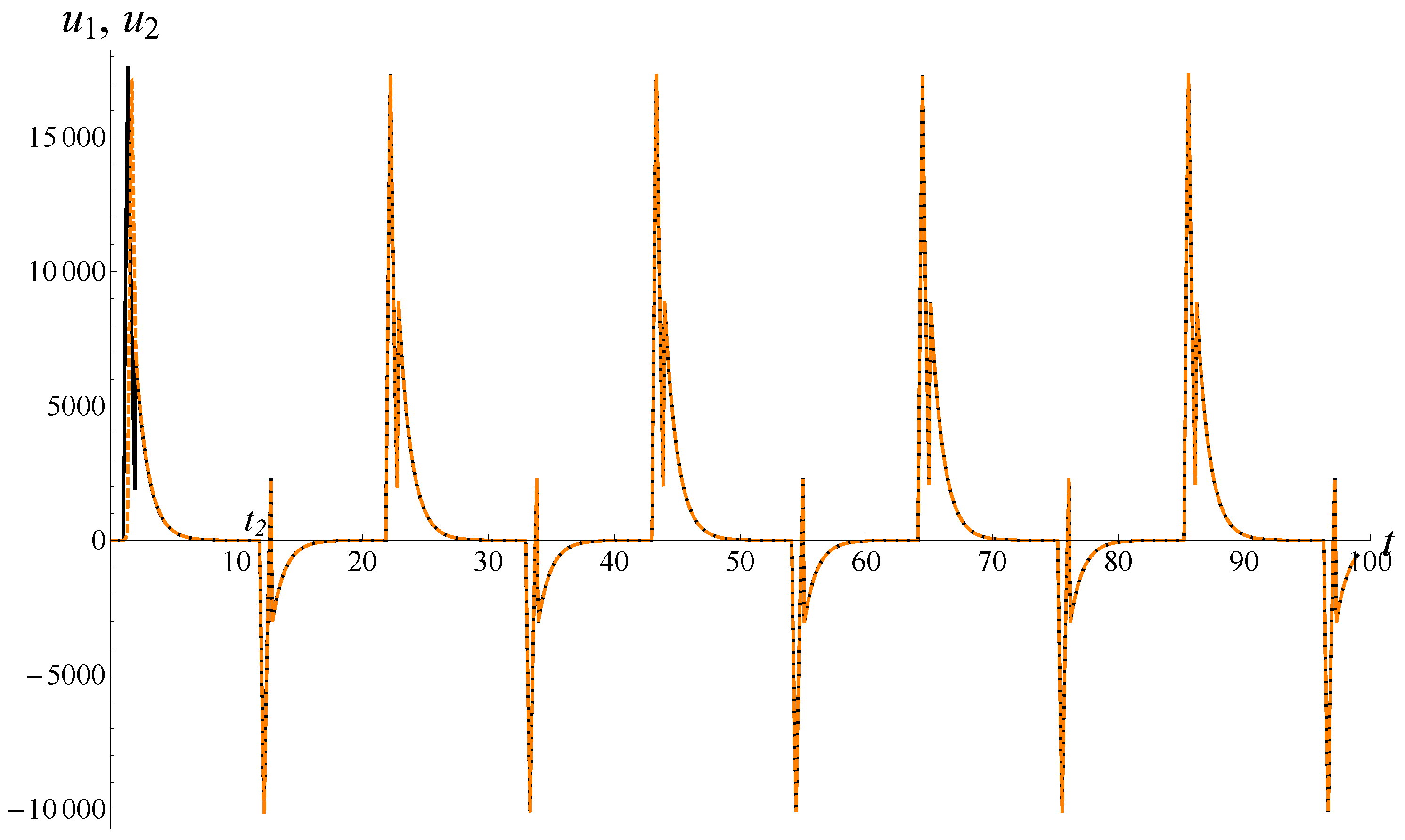
Theorem 1.

Suppose $\gamma >0$ and for values of $k_1$ and $x_1$ Assumptions 1, 2, and inequality (17) hold. Suppose Assumption 3 and inequality (31) hold. Then, for any sufficiently large $\lambda >0$, there exists $t_2=t_2(k_1,x_1)>0$ such that for all $t>t_2$ solution of system (3) satisfies Formulas (29), (30), and (32).

In Figure 1, an example of a solution of system (3) in the case of $\gamma >0$ is shown.

Figure 1. Example of solution. Values of parameters: $T=1$, $\gamma =0.1$, $p=1$, $\lambda$ = 10,000. Black line—$u_1\left(t\right)$, orange dashed line—$u_2\left(t\right)$.

Since F is smooth and $x_{n+1}-k_{n+1}=O\left({\lambda }^{-2\gamma }\right)$ at $\lambda \to +\infty$, then, in the case $\gamma >\frac{1}{2}$, we have the following statement.

Corollary 4.

Suppose $\gamma >\frac{1}{2}$ and for values $k_1$ and $x_1$ Assumptions 1 and 2 hold and inequality (17) is true. Suppose Assumption 3 and inequality (31) are true. Then, for any sufficiently large $\lambda >0$, there exists $t_2(k_1,x_1)>0$ such that for all $t>t_2$ inequality $|u_1\left(t\right)-u_2\left(t\right)|=o\left(1\right)$ is true.

4. Dynamics in the Case of Negative Coupling

In this section, we assume that $-\frac{1}{2}<\gamma <0$. We construct map on $k_n$, $x_n$, and $i_n$ for these values of $\gamma$ and make conclusions about dynamics of system (3).

Suppose inequality

$$D\left(n\right)\ne 0$$

(33)

and Assumptions 1 and 2 for values $k_n$, $x_n$, and $t_n$ hold for all $n\in \mathbb{N}$. Then, like in Section 2, we obtain that, in the case $-\frac{1}{2}<\gamma <0$, values $u_i\left(t_{n+1}\right)$ and $u_{3-i}\left(t_{n+1}\right)$ have the form

$$\begin{array}{c}{u}_i\left(t_{n+1}\right)=\frac{\lambda }{4}(D\left(n\right)+o\left(1\right))e^{-(1+2\gamma )(t_{n+1}-t_n-2T)},\\ u_{3-i}\left(t_{n+1}\right)=\frac{\lambda }{4}(-D\left(n\right)+o\left(1\right))e^{-(1+2\gamma )(t_{n+1}-t_n-2T)}.\end{array}$$

Thus, we obtain that, in the case of negative coupling,

$$t_{n+1}-t_n=\left(\frac{1}{1+2\gamma }+o\left(1\right)\right)ln\lambda$$

(34)

at $\lambda \to +\infty$. It follows from (12) and (34) that the mapping on $k_n$, $x_n$, and $i_n$ has form

$$\begin{array}{c}{k}_{n+1}=\left\{\begin{array}{c}sign\left(D\right(n\left)\right),sign\left(C\right(n\left)D\right(n\left)\right)=-1,\hfill \\ -sign\left(D\right(n\left)\right),sign\left(C\right(n\left)D\right(n\left)\right)=1,\hfill \end{array}\right.\hfill \\ i_{n+1}=\left\{\begin{array}{c}{i}_n,sign\left(C\left(n\right)D\left(n\right)\right)=-1,\hfill \\ 3-i_n,sign\left(C\left(n\right)D\left(n\right)\right)=1,\hfill \end{array}\right.\hfill \\ x_{n+1}=-k_{n+1}+O\left({\lambda }^{\frac{2\gamma }{1+2\gamma }}\right),\hfill \end{array}$$

(35)

at $\lambda \to +\infty$.

Thus, under Assumptions 1, 2 and (33) on the n-th (where $n\ge 2$) iteration of mapping, we have $k_n+x_n=o\left(1\right)$ at $\lambda \to +\infty$. Thus, starting from the second iteration, Assumption 1 should be satisfied for $k=k_n$, $x=-k_n+o\left(1\right)$, and $t_1=t_n$. Let’s formulate this assumption for these values of parameters. Functions $A(k_n,-k_n+o\left(1\right),t,t_n)$ and $B(k_n,-k_n+o\left(1\right),t,t_n)$ have the form

$$\begin{array}{c}A(k_n,-k_n+o\left(1\right),t,t_n)=\underset{T+t_n}{\overset{t}{\int }}(e^{s-t}+e^{(1+2\gamma )(s-t)})F\left(k_{n}p{e}^{(1+2\gamma )(t_n+T-s)}\right)ds\\ +\underset{T+t_n}{\overset{t}{\int }}(e^{s-t}-e^{(1+2\gamma )(s-t)})F(-k_{n}p{e}^{(1+2\gamma )(t_n+T-s)})ds+o\left(1\right),\end{array}$$

$$\begin{array}{c}B(k_n,-k_n+o\left(1\right),t,t_n)=\underset{T+t_n}{\overset{t}{\int }}(e^{s-t}-e^{(1+2\gamma )(s-t)})F\left(k_{n}p{e}^{(1+2\gamma )(t_n+T-s)}\right)ds\\ +\underset{T+t_n}{\overset{t}{\int }}(e^{s-t}+e^{(1+2\gamma )(s-t)})F(-k_{n}p{e}^{(1+2\gamma )(t_n+T-s)})ds+o\left(1\right).\end{array}$$

Value t in Assumption 1 on the n-th iteration of steps described in Section 2 is in the segment $[t_n+T,t_n+2T]$; therefore, for each step value, $\tilde{t}=t-t_n$ is in the segment $[T,2T]$. Note that

$$\begin{array}{c}\underset{T+t_n}{\overset{t}{\int }}(e^{s-t}+e^{(1+2\gamma )(s-t)})F\left(k_{n}p{e}^{(1+2\gamma )(t_n+T-s)}\right)ds\\ +\underset{T+t_n}{\overset{t}{\int }}(e^{s-t}-e^{(1+2\gamma )(s-t)})F(-k_{n}p{e}^{(1+2\gamma )(t_n+T-s)})ds\\ =\underset{T}{\overset{\tilde{t}}{\int }}\left(e^{s-\tilde{t}}+e^{(1+2\gamma )(s-\tilde{t})}\right)F\left(k_{n}p{e}^{(1+2\gamma )(T-s)}\right)ds+\underset{T}{\overset{\tilde{t}}{\int }}\left(e^{s-\tilde{t}}-e^{(1+2\gamma )(s-\tilde{t})}\right)F(-k_{n}p{e}^{(1+2\gamma )(T-s)})ds\end{array}$$

and

$$\begin{array}{c}\underset{T+t_n}{\overset{t}{\int }}(e^{s-t}-e^{(1+2\gamma )(s-t)})F\left(k_{n}p{e}^{(1+2\gamma )(t_n+T-s)}\right)ds\\ +\underset{T+t_n}{\overset{t}{\int }}(e^{s-t}+e^{(1+2\gamma )(s-t)})F(-k_{n}p{e}^{(1+2\gamma )(t_n+T-s)})ds\\ =\underset{T}{\overset{\tilde{t}}{\int }}\left(e^{s-\tilde{t}}-e^{(1+2\gamma )(s-\tilde{t})}\right)F\left(k_{n}p{e}^{(1+2\gamma )(T-s)}\right)ds+\underset{T}{\overset{\tilde{t}}{\int }}\left(e^{s-\tilde{t}}+e^{(1+2\gamma )(s-\tilde{t})}\right)F(-k_{n}p{e}^{(1+2\gamma )(T-s)})ds.\end{array}$$

Thus, for each $n=2,3,\dots$, Assumption 1 is the same (only $k_n$ may change). Thus, if the following assumption holds, then Assumption 1 holds for all $n=2,3,\dots$.

Assumption 4.

Number of points $t^{*}\in [T,2T]$ such that $g_1(k,t^{*})=0$ ($g_2(k,t^{*})=0$) is finite. If $g_1(k,t^{*})=0$ ($g_2(k,t^{*})=0$), then there exists $j\in \mathbb{N}$ such that ${\displaystyle \frac{{\partial }^j{g}_1(k,\tilde{t})}{\partial {\tilde{t}}^j}}{|}_{\tilde{t}=t^{*}}$ (${\displaystyle \frac{{\partial }^j{g}_2(k,\tilde{t})}{\partial {\tilde{t}}^j}}{|}_{\tilde{t}=t^{*}}$, respectively) is non-zero. Here, $k=1$ or $k=-1$ and

$$\begin{array}{c}{g}_1(k,\tilde{t})=\underset{T}{\overset{\tilde{t}}{\int }}\left(e^{s-\tilde{t}}+e^{(1+2\gamma )(s-\tilde{t})}\right)F\left(kp{e}^{(1+2\gamma )(T-s)}\right)ds\\ +\underset{T}{\overset{\tilde{t}}{\int }}\left(e^{s-\tilde{t}}-e^{(1+2\gamma )(s-\tilde{t})}\right)F(-kp{e}^{(1+2\gamma )(T-s)})ds,\end{array}$$

$$\begin{array}{c}{g}_2(k,\tilde{t})=\underset{T}{\overset{\tilde{t}}{\int }}\left(e^{s-\tilde{t}}-e^{(1+2\gamma )(s-\tilde{t})}\right)F\left(kp{e}^{(1+2\gamma )(T-s)}\right)ds\\ +\underset{T}{\overset{\tilde{t}}{\int }}\left(e^{s-\tilde{t}}+e^{(1+2\gamma )(s-\tilde{t})}\right)F(-kp{e}^{(1+2\gamma )(T-s)})ds.\end{array}$$

Thus, under Assumption 4, the asymptotics of the solution has form

$$\begin{array}{c}{u}_{i_n}\left(t\right)=k_{n}p{e}^{-(1+2\gamma )(t-t_n)}+o\left(1\right),\\ u_{3-i_n}\left(t\right)=-k_{n}p{e}^{-(1+2\gamma )(t-t_n)}+o\left(1\right)\end{array}$$

(36)

on the segments $t\in [t_n,t_n+T]$ ((36) is Formula (9) with $i=i_n$, $k=k_n$, $x=x_n=-k_n+o\left(1\right)$, and $t_1=t_n$). On the segments, the $t\in [t_n+T,t_n+2T]$ solution satisfies equalities

$$\begin{array}{c}{u}_{i_n}\left(t\right)=\frac{\lambda }{2}\left(g_1(k_n,t-t_n)+o\left(1\right)\right),\\ u_{3-i_n}\left(t\right)=\frac{\lambda }{2}\left(g_2(k_n,t-t_n)+o\left(1\right)\right)\end{array}$$

(37)

((37) is Formula (10) with $i=i_n$, $k=k_n$, $x=x_n=-k_n+o\left(1\right)$, and $t_1=t_n$, where functions A and B are rewritten in terms of functions $g_1$ and $g_2$).

Suppose that the following non-degeneracy condition holds:

$$\begin{array}{c}{g}_1(1,2T)g_1(-1,2T)g_2(1,2T)g_2(-1,2T)\ne 0,\\ g_1(1,2T)\ne g_2(1,2T),\\ g_1(-1,2T)\ne g_2(-1,2T),\end{array}$$

(38)

(the fulfillment of these inequalities leads to fulfillment of Assumption 2 and inequality (33) for all $n=2,3,\dots$). Thus, under condition (38) on the segments $t\in [t_n+2T,t_{n+1}]$, we have the following asymptotics of solution:

$$\begin{array}{c}{u}_{i_n}\left(t\right)=\frac{\lambda }{2}\left(\underset{T}{\overset{2T}{\int }}{e}^s\left(F\left(k_{n}p{e}^{(1+2\gamma )(T-s)}\right)+F\left(-k_{n}p{e}^{(1+2\gamma )(T-s)}\right)\right)ds+o\left(1\right)\right)e^{t_n-t}\\ +\frac{\lambda }{2}\left(\underset{T}{\overset{2T}{\int }}{e}^{(1+2\gamma )s}\left(F\left(k_{n}p{e}^{(1+2\gamma )(T-s)}\right)-F\left(-k_{n}p{e}^{(1+2\gamma )(T-s)}\right)\right)ds+o\left(1\right)\right)e^{(1+2\gamma )(t_n-t)},\\ u_{3-i_n}\left(t\right)=\frac{\lambda }{2}\left(\underset{T}{\overset{2T}{\int }}{e}^s\left(F\left(k_{n}p{e}^{(1+2\gamma )(T-s)}\right)+F\left(-k_{n}p{e}^{(1+2\gamma )(T-s)}\right)\right)ds+o\left(1\right)\right)e^{t_n-t}\\ -\frac{\lambda }{2}\left(\underset{T}{\overset{2T}{\int }}{e}^{(1+2\gamma )s}\left(F\left(k_{n}p{e}^{(1+2\gamma )(T-s)}\right)-F\left(-k_{n}p{e}^{(1+2\gamma )(T-s)}\right)\right)ds+o\left(1\right)\right)e^{(1+2\gamma )(t_n-t)}\end{array}$$

(39)

((39) is Formula (12) with $i=i_n$, $k=k_n$, $x=x_n=-k_n+o\left(1\right)$, and $t_1=t_n$, where functions A and B are rewritten in terms of function F).

We obtain the following result on dynamics of system (3).

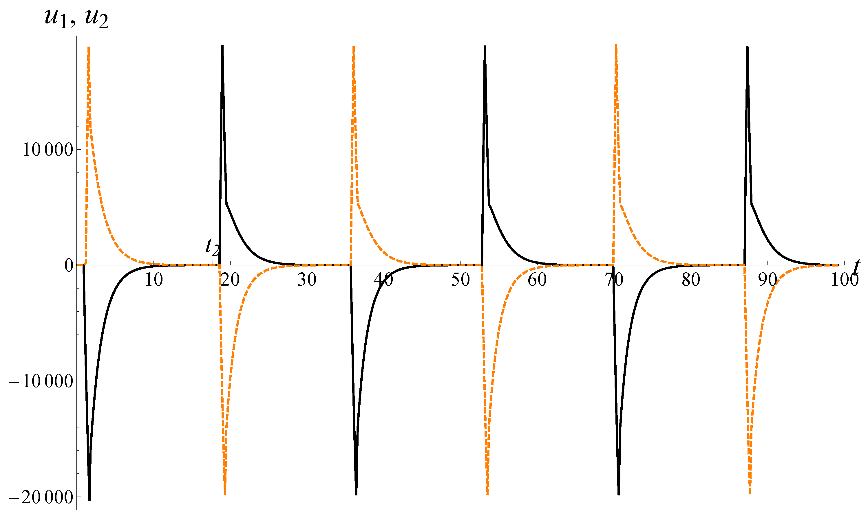
Theorem 2.

Suppose $-\frac{1}{2}<\gamma <0$ and for values of $k_1$ and $x_1$ Assumptions 1, 2, and inequality (20) hold. Suppose Assumption 4 and inequalities (38) hold. Then, for any sufficiently large $\lambda >0$, there exists $t_2=t_2(k_1,x_1)>0$ such that for all $t>t_2$ solution of system (3) satisfies Formulas (36), (37), and (39).

In Figure 2, an example of the solution in the case of $-\frac{1}{2}<\gamma <0$ is shown.

Figure 2. Example of solution. Values of parameters: $T=0.9$, $\gamma =-0.2$, $p=1$, $\lambda$ = 10,000. Black line—$u_1\left(t\right)$, orange dashed line—$u_2\left(t\right)$.

5. Example

In this section, we show how method described in Section 2, Section 3 and Section 4 works in the case when function f satisfies conditions (4) and inequality

$$uf\left(u\right)>0 \mathrm{i}\mathrm{f} 0<\left|u\right|<p$$

(40)

and initial conditions satisfy inequalities

$$\begin{array}{c}kx>0 \mathrm{i}\mathrm{f} \gamma >0,\\ kx<0 \mathrm{i}\mathrm{f} -\frac{1}{2}<\gamma <0\end{array}$$

(41)

(here k and x are defined as in Section 2).

As in Section 2, we construct asymptotics of all solutions of system (3) with initial conditions outside of the strip $|u_j|<p$ ($j=1,2$) and satisfying inequality (41). Let $t_1$ and i be defined as in Section 2. Then, the following lemmas hold.

Lemma 3.

If initial conditions fulfill (41), then functions $u_i\left(t\right)$ and $u_{3-i}\left(t\right)$ do not change their signs on the segment $t\in [t_1,t_1+T]$ and for all $t\in [t_1,t_1+T]$ inequalities

$$\begin{array}{c}{u}_i\left(t\right)u_{3-i}\left(t\right)>0 if\gamma >0,\\ u_i\left(t\right)u_{3-i}\left(t\right)<0 if-\frac{1}{2}<\gamma <0\end{array}$$

(42)

hold.

Proof. 

Consider the case $k=1$. If $\gamma >0$, then $x\ge 1>0$. For these values of k, x, and $\gamma$ system of inequalities,

$$\left\{\begin{array}{c}|k+x|>|x-k|,\hfill \\ e^{-(t-t_1)}\ge e^{-(1+2\gamma )(t-t_1)}\hfill \end{array}\right.$$

(43)

holds. Since $u_i\left(t\right)$ and $u_{3-i}\left(t\right)$ have form (9), $k+x>0$ and (43) holds, then we get that

$$u_i\left(t\right)>0,u_{3-i}\left(t\right)>0$$

(44)

on the interval $t\in [t_1,t_1+T]$. If $-\frac{1}{2}<\gamma <0$, then $x\le -1<0$. This is why we obtain that

$$\left\{\begin{array}{c}|k+x|<|x-k|,\hfill \\ e^{-(t-t_1)}\le e^{-(1+2\gamma )(t-t_1)}.\hfill \end{array}\right.$$

(45)

It follows from (9), $k-x>0$, and (45) that

$$u_i\left(t\right)>0,u_{3-i}\left(t\right)<0$$

(46)

on the interval $t\in [t_1,t_1+T]$.

Consider the case $k=-1$. If $\gamma >0$, then $x\le -1<0$. Then, from (9), $k+x<0$, and (43), we obtain that

$$u_i\left(t\right)<0,u_{3-i}\left(t\right)<0$$

(47)

on the interval $t\in [t_1,t_1+T]$. In addition, in the case $-\frac{1}{2}<\gamma <0$, we get that $x\ge 1>0$ and from (9), $k-x>0$, and (45), we get

$$u_i\left(t\right)<0,u_{3-i}\left(t\right)>0$$

(48)

on the interval $t\in [t_1,t_1+T]$.

It follows from (44), (46)–(48) that inequalities (42) hold. □

Lemma 4.

If function $u_i\left(t\right)$ comes into the strip $|u_i\left(t\right)|<p$ at the point $t=t_1$, then (1) x satisfies inequality

$$\left|x\right|\le |1+1/\gamma |;$$

(49)

(2) function $u_i$ is in the strip $|u_i\left(t\right)|<p$ for all $t\in (t_1,t_1+T]$.

Proof. 

It follows from (9) that

$$u_i^{\prime }\left(t\right)=-\frac{(k+x)p}{2}{e}^{-(t-t_1)}-(1+2\gamma )\frac{(k-x)p}{2}{e}^{-(1+2\gamma )(t-t_1)},$$

(50)

therefore

$$u_i^{\prime }\left(t_1\right)=-\left(\frac{k+x}{2}p+(1+2\gamma )\frac{k-x}{2}p\right).$$

Consider the case $k=1$. For $k=1$ value, $u_i\left(t_1\right)$ is equal to p. If this function comes into the strip $|u_i\left(t\right)|<p$ at the point $t=t_1$, then derivative $u_i^{\prime }\left(t_1\right)$ is non-positive. For $k=1$ inequality, $u_i^{\prime }\left(t_1\right)\le 0$ is equivalent to $1+\gamma \ge \gamma x$. It follows from condition (41) that $\gamma x>0$ in the case $k=1$. Thus, in the case $k=1$, inequality (49) holds.

Consider the case $k=-1$. For $k=-1$ value $u_i\left(t_1\right)=-p$ and if this function comes into the strip $|u_i\left(t\right)|<p$ at the point $t=t_1$, then derivative $u_i^{\prime }\left(t_1\right)$ is non-negative. For $k=-1$ condition, $u_i^{\prime }\left(t_1\right)\ge 0$ is equivalent to inequality $-1-\gamma \le \gamma x$. From (41), we get that $\gamma x<0$, so inequality (49) is true in this case, too.

It follows from (41) and (49) that in the case $\gamma >0$ system of inequalities

$$\left\{\begin{array}{c}|k+x|\ge \left|\right(1+2\gamma \left)\right(x-k\left)\right|,\hfill \\ e^{-(t-t_1)}>e^{-(1+2\gamma )(t-t_1)}\hfill \end{array}\right.$$

(51)

holds and in the case $-\frac{1}{2}<\gamma <0$ system of inequalities

$$\left\{\begin{array}{c}|k+x|\le \left|\right(1+2\gamma \left)\right(x-k\left)\right|,\hfill \\ e^{-(t-t_1)}<e^{-(1+2\gamma )(t-t_1)}\hfill \end{array}\right.$$

(52)

is true on the interval $t\in (t_1,t_1+T]$

Using (50)–(52), and (41), we obtain that

$$\begin{array}{c}{u}_i^{\prime }\left(t\right)<0 \mathrm{i}\mathrm{f} k=1,\\ u_i^{\prime }\left(t\right)>0 \mathrm{i}\mathrm{f} k=-1\end{array}$$

(53)

on the interval $t\in (t_1,t_1+T]$. Combining (44), (46)–(48) with (53), we get that function $u_i\left(t\right)$ is in the strip $|u_i\left(t\right)|<p$ for all $t\in (t_1,t_1+T]$. □

Lemma 5.

If function f satisfies (4) and (40), initial conditions satisfy (41) and

$$\left|x\right|<|1+1/\gamma |,$$

(54)

then Assumptions 1–4 hold.

Proof. 

Consider some function $f\left(u\right)$, satisfying conditions (4) and (40).

Let us prove that for this function Assumption 1 holds. From Lemmas 3 and 4, we obtain that $u_i\left(t\right)$ is in the strip $|u_i\left(t\right)|<p$ and it does not change sign on the interval $t\in (t_1,t_1+T]$. This is why from condition (40) we get that the first summands in $A(k,x,t,t_1)$ and $B(k,x,t,t_1)$ are non-zero. Thus, from formulas (44), (46)–(48), and assumption (40), we obtain that the following inequalities hold

$$\begin{array}{ccc}A(k,x,t,t_1)>0,B(k,x,t,t_1)>0\hfill & \mathrm{i}\mathrm{f}& \hfill k=1,\gamma >0\\ A(k,x,t,t_1)>0,B(k,x,t,t_1)<0\hfill & \mathrm{i}\mathrm{f}& \hfill k=1,-\frac{1}{2}<\gamma <0\\ A(k,x,t,t_1)<0,B(k,x,t,t_1)<0\hfill & \mathrm{i}\mathrm{f}& \hfill k=-1,\gamma >0\\ A(k,x,t,t_1)<0,B(k,x,t,t_1)>0\hfill & \mathrm{i}\mathrm{f}& \hfill k=-1,-\frac{1}{2}<\gamma <0\end{array}$$

(55)

on the interval $t\in (t_1+T,t_1+2T]$. Thus, we have proved that under condition (40) functions $A(k,x,t,t_1)$ and $B(k,x,t,t_1)$ are non-zero on the interval $t\in (t_1+T,t_1+2T]$. If $t^{*}=t_1+T$, then $A(k,x,t^{*},t_1)=B(k,x,t^{*},t_1)=0$. Derivatives ${\displaystyle \frac{{\partial }^{j}A(k,x,t,t_1)}{\partial t^j}}{|}_{t=t_1+T}=0$ for $j=1,2$ and derivatives ${\displaystyle \frac{{\partial }^{j}B(k,x,t,t_1)}{\partial t^j}}{|}_{t=t_1+T}=0$ for $j=1,2,3$. Expressions

$${\displaystyle \frac{{\partial }^{3}A(k,x,t,t_1)}{\partial t^3}}{|}_{t=t_1+T}=2f^{″}\left(kp\right){\left(\frac{k+x}{2}p+(1+2\gamma )\frac{k-x}{2}p\right)}^2$$

and

$${\displaystyle \frac{{\partial }^{4}B(k,x,t,t_1)}{\partial t^4}}{|}_{t=t_1+T}=2\gamma f^{″}\left(kp\right){\left(\frac{k+x}{2}p+(1+2\gamma )\frac{k-x}{2}p\right)}^2,$$

are non-zero: under condition (54) last factor in these derivatives is non-zero and $f^{″}\left(kp\right)\ne 0$ because of (4) (if $x=\pm (1+1/\gamma )$, then for all $j\in \mathbb{N}$ expressions ${\displaystyle \frac{{\partial }^{j}A(k,x,t,t_1)}{\partial t^j}}{|}_{t=t_1+T}$ and ${\displaystyle \frac{{\partial }^{j}B(k,x,t,t_1)}{\partial t^j}}{|}_{t=t_1+T}$ equal zero). Consequently, Assumption 1 holds under condition (54). This assumption holds for $x=\pm k+o\left(1\right)$ at $\lambda \to +\infty$, so Assumptions 3 and 4 hold.

Since the system of inequalities (55) is true for $t=t_1+2T$, then Assumption 2 holds. □

Note that if function $u_i\left(t\right)$ comes to the strip $|u_i\left(t\right)|<p$, then x satisfies inequality (49), and for all x such that (54) hold, Assumption 1 is true. Thus, only for two values of parameter $x:$$x_{1,2}=\pm (1+1/\gamma )$ is Assumption 1 false.

Lemma 6.

If function f satisfies (4) and (40), then inequalities (26) and (31) are true in the case $\gamma >0$ and inequalities (33) and (38) hold in the case $-\frac{1}{2}<\gamma <0$.

Proof. 

It follows from Lemma 5 that $A(k,x,t_1+2T,t_1)$ and $B(k,x,t_1+2T,t_1)$ have the same sign in the case $\gamma >0$ and the opposite signs in the case $-\frac{1}{2}<\gamma <0$. Therefore, in the case $\gamma >0$ ($-\frac{1}{2}<\gamma <0$) inequality (26) (inequality (33) respectively) holds for all $n=1,2,3,\dots$. Thus, inequalities (31) and (38) are fulfilled because they are equivalent to Assumption 2 and conditions (26) and (33) for $n=2,3,\dots$. □

Thus, we have proved that all assumptions in Theorems 1 and 2 are true if function f satisfies (4) and (40) and for $x_1$ conditions (41) and (54) hold. Therefore, for class of functions f considered in this section, the following theorems are true.

Theorem 3.

Suppose $\gamma >0$ and inequalities (41) and $x_1\ne \pm (1+1/\gamma )$ hold. Then, for any sufficiently large $\lambda >0$ there exists $t_2=t_2(k_1,x_1)>0$ such that for all $t>t_2$ solution of system (3) satisfies Formulas (29), (30) and (32).

Theorem 4.

Suppose $-\frac{1}{2}<\gamma <0$ and inequalities (41) and $x_1\ne \pm (1+1/\gamma )$ hold. Then, for any sufficiently large $\lambda >0$ there exists $t_2=t_2(k_1,x_1)>0$ such that for all $t>t_2$ solution of system (3) satisfies Formulas (36), (37) and (39).

Remark 1.

If $x_1=\pm (1+1/\gamma )$, then Assumption 1 is not true, so Theorems 3 and 4 are not proven. However, probably, they are true because for all initial conditions in the neighborhood of these values they are true.

Consider the map (28). If we take set $\left\{1\right\}\times [1,1+1/\gamma -\delta ]$ (where $\delta$ is a small positive constant ($0<\delta <1/\gamma$)) of pairs $(k,x)$, then it follows from Lemmas 3–6 that the image of this set under the map (28) is set $\left\{1\right\}\times [1,1+a]$, where $a=o\left(1\right)$ at $\lambda \to +\infty$. Therefore, there exists at least one fixed point of the operator of translation along the trajectories and positive relaxation cycle of system (3) corresponds to this fixed point (if $k_1$ and $x_1$ fulfill (41) and function f satisfies (40), then in the case of positive coupling solution of system (3) does not change its sign). Similarly, there exists at least one negative relaxation cycle of system (3) in the case of positive coupling.

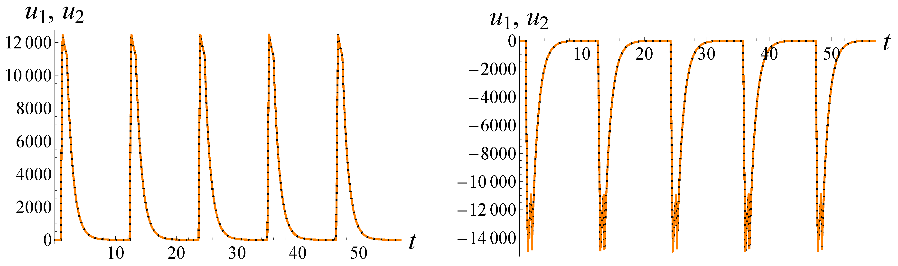
In Figure 3, there are examples of two coexisting relaxation cycles of system (3).

Figure 3. Two coexisting relaxation cycles of the system (3). Values of parameters: $T=1$, $\gamma =0.4$, $p=1$, $\lambda$ = 10,000. Black line—$u_1\left(t\right)$, orange dashed line—$u_2\left(t\right)$.

If $-\frac{1}{2}<\gamma <0$, then it follows from (35) that $x_{n+1}=-k_{n+1}+o\left(1\right)$ at $\lambda \to +\infty$. It follows from Lemmas 3–6 that for all $(k_n,x_n)\in \{-1\}\times [1,1+1/\gamma -\delta ]$ and $(k_n,x_n)\in \left\{1\right\}\times [-1-1/\gamma +\delta ,-1]$ Theorem 4 is true. Therefore, there exists at least one $q\in \mathbb{N}$, such that image of the set $\{-1\}\times [1,1+1/\gamma -\delta ]$ (or $\left\{1\right\}\times [-1-1/\gamma +\delta ,-1]$) under the q-th iteration of map (35) belongs to the set $\{-1\}\times [1,1+1/\gamma -\delta ]$ (or $\left\{1\right\}\times [-1-1/\gamma +\delta ,-1]$ respectively). Thus, in the case of $-\frac{1}{2}<\gamma <0$, there exists at least one relaxation cycle.

Thus, the following statement holds.

Corollary 5.

Suppose conditions (4) and (40) are true. Then, in the case $\gamma >0$, there exists at least two relaxation cycles of system (3) and in the case of $-\frac{1}{2}<\gamma <0$ there exists at least one relaxation cycle of system (3).

6. Dependence of Dynamics of System (3) on the Sign of Coupling

In this section, we show how asymptotics and difference $t_{n+1}-t_n$ (analog of period) of solutions of system (3) depends on the value $\gamma$ in the case $\gamma >0$ and in the case $-\frac{1}{2}<\gamma <0$ (in this section below, we discuss only such solutions of system (3) for those assumptions of Theorem 1 or 2 fulfill).

First, consider the case $\gamma >0$. From Formulas (29), (30), and (32), we obtain that components $u_1\left(t\right)$ and $u_2\left(t\right)$ have the same leading terms of asymptotics on the interval $t\in [t_2,+\infty )$ and that these leading terms of asymptotics do not depend on $\gamma$. Thus, from Formulas (9), (10), (12), (29), (30) and (32), we obtain that the leading term of asymptotics of solution of system (3) depends on $\gamma$ only for $t\in [0,t_2]$ (see Figure 4). From Corollary 4, we get that in the case $\gamma >\frac{1}{2}$ difference $u_1\left(t\right)-u_2\left(t\right)$ has order $o\left(1\right)$ at $\lambda \to +\infty$ for all $t\ge t_2$, so we may say that in the case $\gamma >\frac{1}{2}$ oscillators $u_1\left(t\right)$ and $u_2\left(t\right)$ “synchronize” (for smaller values of $\gamma$ oscillators $u_1\left(t\right)$ and $u_2\left(t\right)$ may “synchronize”, too, but in the case $\gamma >\frac{1}{2}$ they must “synchronize”).

Figure 4. Solutions of system (3) for different values of parameter $\gamma$. Values of parameters: $T=2$, $p=1.5$, $\lambda =1000$, $k=1$, $x=3$, (a) $\gamma =0.2$; (b) $\gamma =0.6$; (c) $\gamma =1$; (d) $\gamma =1.5$. Black line—$u_1\left(t\right)$, orange dashed line—$u_2\left(t\right)$.

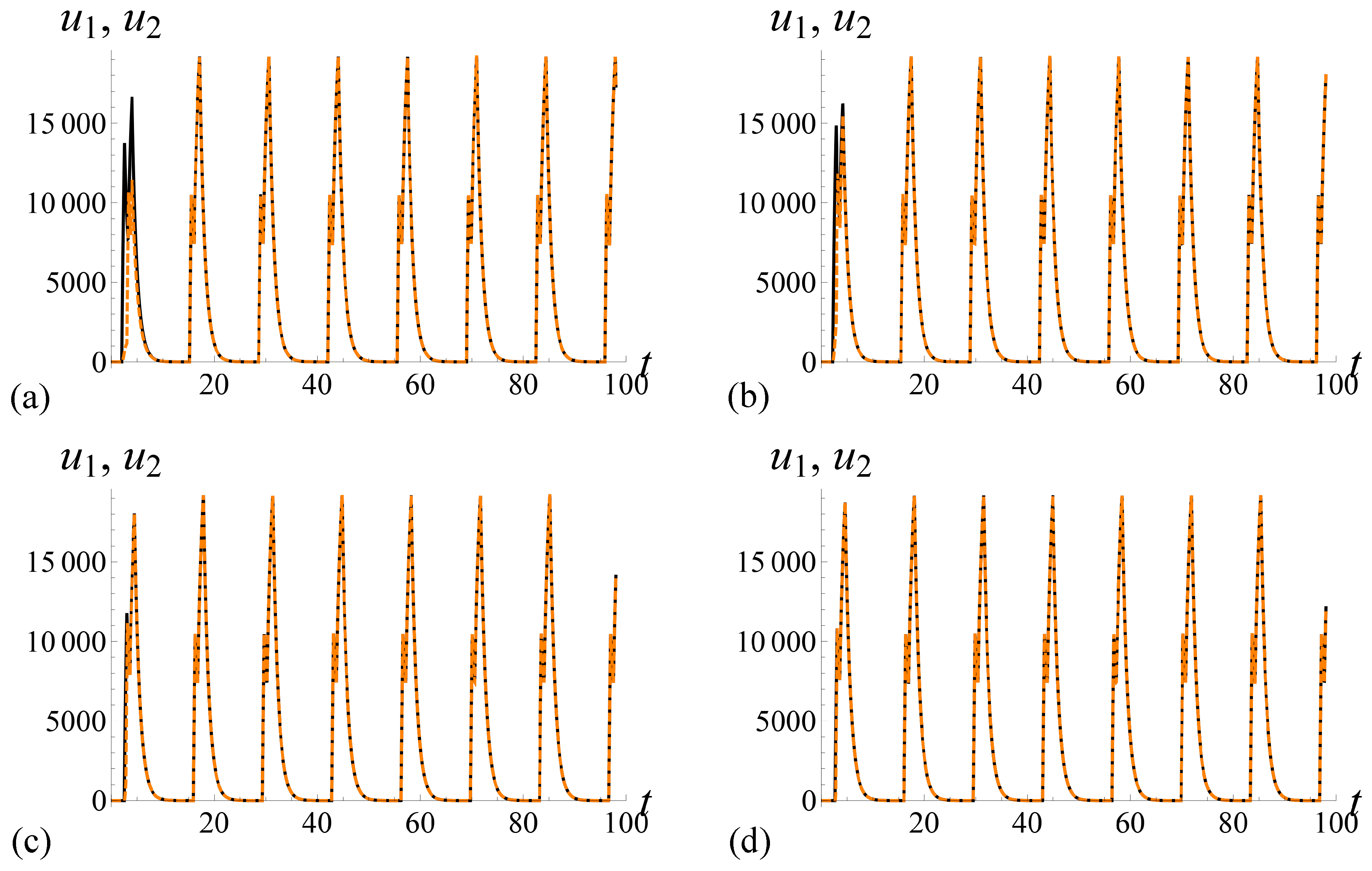
The leading term of asymptotics of the difference $t_{n+1}-t_n$ does not depend on $\gamma$, too.

Figure 4 illustrates dependence of solutions of system (3) on $\gamma$ in the case $\gamma >0$. There are solutions of system (3) with identical function F, parameters $\lambda$ and T, and initial conditions for different parameters $\gamma$ in Figure 4.

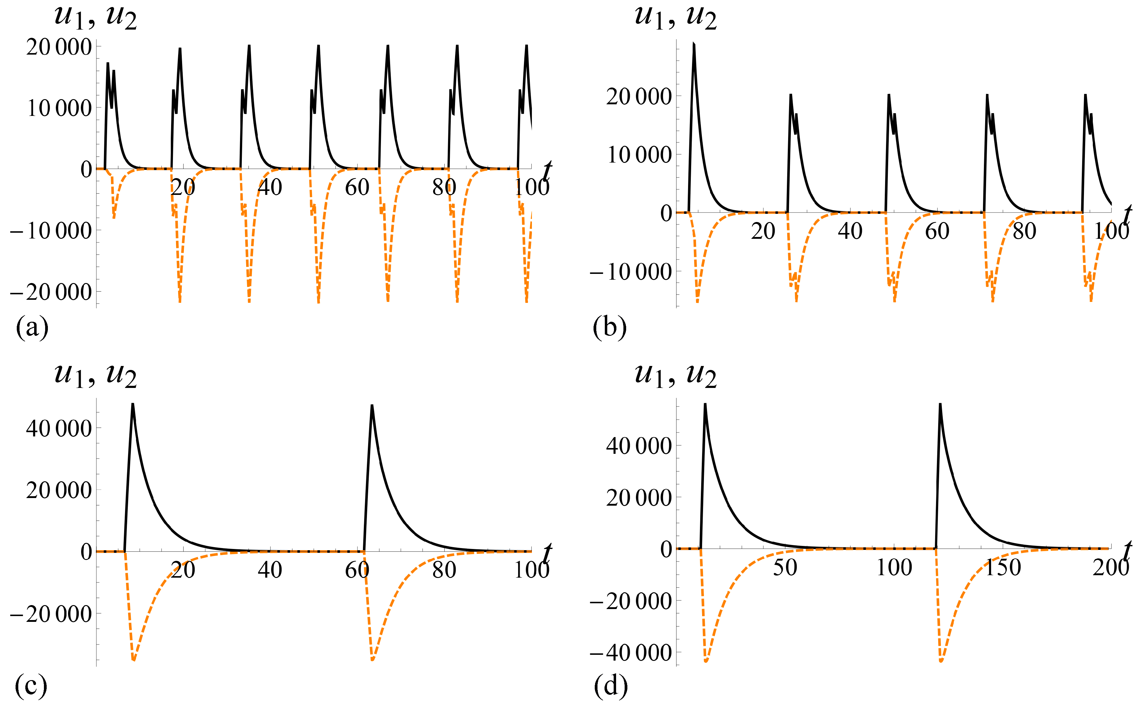
Now, consider the case $-\frac{1}{2}<\gamma <0$.

From (9), (10), (12), (36), (37), and (39), we get that asymptotics of solutions of system (3) depends crucially on the value of parameter $\gamma$ for all $t\ge 0$ in the case $-\frac{1}{2}<\gamma <0$ and that oscillators $u_1\left(t\right)$ and $u_2\left(t\right)$ are not close to each other (the leading terms of their asymptotics are different for all $t\ge t_2$).

It follows from (34) that difference $t_{n+1}-t_n$ increases with the decreasing of parameter $\gamma$ (see Figure 5).

Figure 5. Solutions of system (3) for different values of parameter $\gamma$. Values of parameters: $T=2$, $p=1.5$, $\lambda =1000$, $k=1$, $x=-4$, (a) $\gamma =-0.1$; (b) $\gamma =-0.25$; (c) $\gamma =-0.4$; (d) $\gamma =-0.45$. Black line—$u_1\left(t\right)$, orange dashed line—$u_2\left(t\right)$.

Thus, asymptotics and shape of solution and difference $t_{n+1}-t_n$ depend crucially on the value of $\gamma$ in the case $-\frac{1}{2}<\gamma <0$ (see Figure 5).

Figure 5 illustrates the dependence of solutions of system (3) on $\gamma$ in the case $-\frac{1}{2}<\gamma <0$. Solutions of system (3) with identical function F, parameters $\lambda$ and T, and initial conditions for different parameters $\gamma$ are presented in Figure 5.

7. Conclusions

In this paper, we have studied the nonlocal dynamics of a system of two coupled generators with delayed feedback and dependence of solutions on the value of coupling.

For a wide set of initial conditions from the phase space of system (3) using method of steps and special constructed finite dimensional map, we get asymptotics of relaxation solutions. We obtain relaxation cycles of system (3).

We prove that the dynamics of system (3) are qualitatively different in case $\gamma >0$ and case $-\frac{1}{2}<\gamma <0$: in the case $\gamma >0$, there exists a moment of time $t_2$ after that both components of solution have the same leading term of asymptotics and this leading term does not depend on $\gamma$ if $t>t_2$, generators $u_1\left(t\right)$ and $u_2\left(t\right)$ “synchronize” if $\gamma >\frac{1}{2}$; in the case of $-\frac{1}{2}<\gamma <0$, the leading term of asymptotics and shape of solution depend on $\gamma$, oscillators $u_1\left(t\right)$ and $u_2\left(t\right)$ are not close to each other; the leading term of asymptotics of the value $t_{n+1}-t_n$ (this value serves us an analog of period) increase with decreasing of the value $\gamma$ in the case $-\frac{1}{2}<\gamma <0$ and remains unchanged with changing $\gamma$ in the case $\gamma >0$.

The method of research used in this paper is applicable for systems of higher dimensions (case of n identically diffusion coupled oscillators, where $n>2$) and for systems of n ($n\ge 2$) coupled oscillators with other types of coupling.