A Generator of Bivariate Distributions: Properties, Estimation, and Applications

Abstract

In 2020, El-Morshedy et al. introduced a bivariate extension of the Burr type X generator (BBX-G) of distributions, and Muhammed presented a bivariate generalized inverted Kumaraswamy (BGIK) distribution. In this paper, we propose a more flexible generator of bivariate distributions based on the maximization process from an arbitrary three-dimensional baseline distribution vector, which is of interest for maintenance and stress models, and expands the BBX-G and BGIK distributions, among others. This proposed generator allows one to generate new bivariate distributions by combining non-identically distributed baseline components. The bivariate distributions belonging to the proposed family have a singular part due to the latent component which makes them suitable for modeling two-dimensional data sets with ties. Several distributional and stochastic properties are studied for such bivariate models, as well as for its marginals, conditional distributions, and order statistics. Furthermore, we analyze its copula representation and some related association measures. The EM algorithm is proposed to compute the maximum likelihood estimations of the unknown parameters, which is illustrated by using two particular distributions of this bivariate family for modeling two real data sets.

1. Introduction

Gumbel [1], Freund [2], and Marshall and Olkin [3] in their pioneering papers developed bivariate exponential distributions. Since then, an extensive amount of work has been done on these models and their different generalizations, which have played a crucial role in the construction of multivariate distributions and modeling in a wide variety of applications, such as physic, economy, biology, health, engineering, computer science, etc. Several continuous bivariate distributions can be found in Balakrishnan and Lai [4], and some generalizations and multivariate extensions have been studied by Franco and Vivo [5], Kundu and Gupta [6], Franco et al. [7], Gupta et al. [8], Kundu et al. [9], among others, and recently by Muhammed [10], Franco et al. [11], and El-Morshedy et al. [12], also see the references cited therein.

Kundu and Gupta [13] introduced a bivariate generalized exponential (BGE) distribution by using the trivariate reduction technique with generalized exponential (GE) random variables, which is based on the maximization process between components with a latent random variable, suitable for modeling of some stress and maintenance models. This procedure has also been applied in the literature to generate other bivariate distributions, for example, the bivariate generalized linear failure rate (BGLFR) given by Sarhan et al. [14], the bivariate log-exponentiated Kumaraswamy (BlogEK) introduced by Elsherpieny et al. [15], the bivariate exponentiated modified Weibull extension (BEMWE) given by El-Gohary et al. [16], the bivariate inverse Weibull (BIW) studied by Muhammed [17] and Kundu and Gupta [18], the bivariate Dagum (BD) provided by Muhammed [19], the bivariate generalized Rayleigh (BGR) depicted by Sarhan [20], the bivariate Gumbel-G (BGu-G) presented by Eliwa and El-Morshedy [21], the bivariate generalized inverted Kumaraswamy (BGIK) given by Muhammed [10], and the bivariate Burr typeX-G (BBX-G) proposed by El-Morshedy et al. [12]. Some associated inferential issues have been discussed in these articles, and all of them are based on considering the same kind of baseline components. In each of these bivariate models, the baseline components belong to the proportional reversed hazard rate (PRH) family with a certain underlying distribution (Gupta et al. [22] and Di Crescenzo [23]). It is worth mentioning that Kundu and Gupta [24] extended the BGE model by using components within the PRH family, called a bivariate proportional reversed hazard rate (BPRH) family, and a multivariate extension of the BPRH model was studied by Kundu et al. [9].

The main aim of this paper is to provide a more flexible generator of bivariate distributions based on the maximization process from an arbitrary three-dimensional baseline continuous distribution vector, i.e., not necessarily identical continuous distributions. Hence, this proposed generator allows researchers and practitioners to generate new bivariate distributions even by combining non-identically distributed baseline components, which may be interpreted as a stress model or as a maintenance model. We refer to the bivariate models from this generator as the generalized bivariate distribution (GBD) family, which contains as special cases the aforementioned bivariate distributions. Note that a two-dimensional random variable $(X_1,X_2)$, belonging to the GBD family, has dependent components due to a latent factor, and its joint cumulative distribution function (cdf) is not absolutely continuous, i.e., the joint cdf is a mixture of an absolutely continuous part and a singular part due to the positive probability of the event $X_1=X_2$, whereas the line $x_1=x_2$ has two-dimensional Lebesgue measure zero. In general, the maximum likelihood estimation (MLE) of the unknown parameters a GBD model cannot be obtained in closed form, and we propose using an EM algorithm to compute the MLEs of such parameters.

The rest of the paper is organized as follows. The construction of the GBD family is given in Section 2, and we obtain its decomposition in absolutely continuous and singular parts and its joint probability density function (pdf). In Section 3, several special bivariate models are presented. The cdf and pdf of the marginals and conditional distributions are derived in Section 4, as well as for its order statistics. Some dependence and two-dimensional ageing properties for the GBD family, and stochastic properties of their marginals and order statistics are studied in Section 5, as well as its copula representation and some related association measures. The EM algorithm is proposed in Section 6, which is applied in Section 7, for illustrative purposes, to find the MLEs of particular models of the GBD family in the analysis of two real data sets. Finally, the multivariate extension is discussed in Section 8, as well as the concluding remarks. Some of the proofs are relegated to Appendix A for a fluent presentation of the results, and some technical details of the applications can be found in Appendix B.

2. The GBD Family

In this section, we define the generalized bivariate distribution family as a generator system from any three-dimensional baseline continuous distribution, and then we provide its joint cdf, decomposition, and joint pdf.

Let $U_1$, $U_2$, and $U_3$ be mutually independent random variables with any continuous distribution functions $F_{U_1}$, $F_{U_2}$ and $F_{U_3}$, respectively. Let $X_1=max(U_1,U_3)$ and $X_2=max(U_2,U_3)$. Then, the random vector $(X_1,X_2)$ is said to be a GBD model with baseline distribution vector $(F_{U_1},F_{U_2},F_{U_3})$.

Theorem 1.

Let $(X_1,X_2)$ be a GBD model with baseline distribution vector $(F_{U_1},F_{U_2},F_{U_3})$, then its joint cdf is given by

$$F(x_1,x_2)=F_{U_1}\left(x_1\right)F_{U_2}\left(x_2\right)F_{U_3}\left(z\right),$$

(1)

where $z=min(x_1,x_2)$, for all $x_1,x_2\in \mathbb{R}$.

Proof. 

It is immediate since

$$\begin{array}{cc}\hfill F(x_1,x_2)& =P(X_1\le x_1,X_2\le x_2)=P(max(U_1,U_3)\le x_1,max(U_2,U_3)\le x_2)\hfill \\ \hfill & =P(U_1\le x_1,U_2\le x_2,U_3\le min(x_1,x_2))=F_{U_1}\left(x_1\right)F_{U_2}\left(x_2\right)F_{U_3}(min(x_1,x_2)).\hfill \end{array}$$

□

For instance, a stress model may lead to the GBD family, as in Kundu and Gupta [13]. Suppose a two-component system where each component is subject to an individual independent stress, say $U_1$ and $U_2$, respectively. The system has an overall stress $U_3$ which has been equally transmitted to both the components, independent of their individual stresses. Then, the observed stress for each component is the maximum of both, individual and overall stresses, i.e., $X_1=max(U_1,U_3)$ and $X_2=max(U_2,U_3)$, and $(X_1,X_2)$ is a GBD model.

Analogously, a GBD model is also plausible for a maintenance model. Suppose a system has two components, and it is assumed that each component has been maintained independently and there is also an overall maintenance. Due to component maintenance, the lifetime of the individual component is increased by a random time, say $U_1$ and $U_2$ respectively, and, because of the overall maintenance, the lifetime of each component is increased by another random time $U_3$. Then, the increased lifetime of each component is the maximum of both individual and overall maintenances, $X_1=max(U_1,U_3)$ and $X_2=max(U_2,U_3)$, respectively.

As mentioned before, a bivariate model belonging to the GBD family does not have an absolutely continuous cdf. Let us see now the decomposition of a GBD model as a mixture of bivariate absolutely continuous and singular cdfs, the proof is provided in Appendix A.

Theorem 2.

Let $(X_1,X_2)$ be a GBD model with baseline distribution vector $(F_{U_1},F_{U_2},F_{U_3})$. Then,

$$F(x_1,x_2)=\alpha F_s(x_1,x_2)+(1-\alpha )F_{ac}(x_1,x_2)$$

(2)

where

$$F_s(x_1,x_2)=\frac{1}{\alpha }{\int }_{-\infty }^z{F}_{U_1}\left(u\right)F_{U_2}\left(u\right)d{F}_{U_3}\left(u\right)$$

(3)

and

$$F_{ac}(x_1,x_2)=\frac{1}{1-\alpha }\left(F_{U_1}\left(x_1\right)F_{U_2}\left(x_2\right)F_{U_3}\left(z\right)-{\int }_{-\infty }^z{F}_{U_1}\left(u\right)F_{U_2}\left(u\right)d{F}_{U_3}\left(u\right)\right)$$

(4)

with $z=min(x_1,x_2)$, are the singular and absolutely continuous parts, respectively, and

$$\alpha ={\int }_{-\infty }^{\infty }{F}_{U_1}\left(u\right)F_{U_2}\left(u\right)d{F}_{U_3}\left(u\right).$$

In addition, due to the singular part $F_s$ in (2), the GBD family does not have a pdf with respect to the two-dimensional Lebesgue measure even when the distribution functions $F_{U_1}$, $F_{U_2}$, and $F_{U_3}$ are absolutely continuous. However, it is possible to construct a joint pdf for $(X_1,X_2)$ through a mixture between a pdf with respect to the two-dimensional Lebesgue measure and a pdf with respect to the one-dimensional Lebesgue measure (the proof is provided in Appendix A).

Theorem 3.

If $(X_1,X_2)$ is a GBD model with joint cdf given by (1), then the joint pdf with respect to μ, the measure associated with F, is

$$f(x_1,x_2)=\left\{\begin{array}{cc}{f}_1(x_1,x_2),\hfill & \mathit{if}{x}_1<x_2\hfill \\ f_2(x_1,x_2),\hfill & \mathit{if}{x}_1>x_2\hfill \\ f_0\left(x\right),\hfill & \mathit{if}{x}_1=x_2=x,\hfill \end{array}\right.$$

where

$$f_i(x_1,x_2)=f_{U_j}\left(x_j\right)\left(f_{U_i}\left(x_i\right)F_{U_3}\left(x_i\right)+F_{U_i}\left(x_i\right)f_{U_3}\left(x_i\right)\right),withi\ne j\in \{1,2\},$$

and

$$f_0\left(x\right)=f_{U_3}\left(x\right)F_{U_1}\left(x\right)F_{U_2}\left(x\right),$$

when the pdf $f_{U_i}$ of $U_i$ exists, $i=1,2,3$.

3. Special Cases

In this section, we derive new bivariate models from Theorem 1, taking into account particular baseline distribution vectors $(F_{U_1},F_{U_2},F_{U_3})$.

Note that, if the baseline components $U_i$s belong to the same distribution family, say $F_U$, then the proposed generator provides novel extended bivariate versions of that distribution $F_U$. Furthermore, under certain restrictions on the underlying parameters of each $U_i$, bivariate distributions given in the literature are obtained. From now on, it is assumed that all parameters of each $F_{U_i}$ are positive unless otherwise mentioned.

Extended bivariate generalized exponential model. A random variable U follows a GE distribution, $U\sim GE(\theta ,\lambda )$ (see Gupta and Kundu [25]), if its cdf is given by

$$F_{GE}(u;\theta ,\lambda )={\left(1-e^{-\lambda u}\right)}^{\theta },\mathrm{for}u>0.$$

If $U_i\sim GE({\theta }_i,{\lambda }_i)$ $i=1,2,3$, then the GBD model with the GE baseline distribution vector is an extended BGE model with $\mathit{\theta }=({\theta }_1,{\theta }_2,{\theta }_3)$ and $\mathit{\lambda }=({\lambda }_1,{\lambda }_2,{\lambda }_3)$ parameter vectors, denoted as $(X_1,X_2)\sim EBGE(\mathit{\theta },\mathit{\lambda })$, and its joint cdf is

$$F_{EBGE}(x_1,x_2)=F_{GE}(x_1;{\theta }_1,{\lambda }_1)F_{GE}(x_2;{\theta }_2,{\lambda }_2)F_{GE}(z;{\theta }_3,{\lambda }_3),\mathrm{for}{x}_1>0,x_2>0,$$

where $z=min(x_1,x_2)$.

As a particular case, if $\lambda ={\lambda }_i$, $i=1,2,3$, $(X_1,X_2)\sim BGE(\mathit{\theta },\lambda )$ given by Kundu and Gupta [13].

Extended bivariate proportional reversed hazard rate model. If $U_i\sim PRH\left({\theta }_i\right)$ with base distribution $F_{B_i}$ $i=1,2,3$, i.e., its cdf can be expressed as $F_{U_i}=F_{B_i}^{{\theta }_i}$ (see Gupta et al. [22] and Di Crescenzo [23]), then the GBD model with PRH baseline distribution vector provides an extended BPRH model, $(X_1,X_2)\sim EBPRH(\mathit{\theta },\mathit{\lambda })$, with $\mathit{\theta }=({\theta }_1,{\theta }_2,{\theta }_3)$ parameter vector of the PRH components and $\mathit{\lambda }=({\lambda }_1,{\lambda }_2,{\lambda }_3)$ parameter vector of the underlying distributions $F_{B_i}$’s. From (1), its joint cdf is given by

$$F_{EBPRH}(x_1,x_2)=F_{B_1}^{{\theta }_1}(x_1;{\lambda }_1)F_{B_2}^{{\theta }_2}(x_2;{\lambda }_2)F_{B_3}^{{\theta }_3}(z;{\lambda }_3),\mathrm{for}{x}_1>0,x_2>0,$$

where $z=min(x_1,x_2)$.

In particular, if the PRH components have the same base distribution, $F_B=F_{B_i}$ $i=1,2,3$, then $(X_1,X_2)\sim BPRH(\mathit{\theta },\lambda )$ with baseline distribution $F_B(·;\lambda )$ introduced by Kundu and Gupta [24].

Extended bivariate generalized linear failure rate model. It is said that a random variable U follows a GLFR distribution, $U\sim GLFR(\theta ,\lambda ,\gamma )$ (see Sarhan and Kundu [26]), if its cdf is given by

$$F_{GLFR}(u;\theta ,\lambda ,\gamma )={\left(1-exp\left(-\lambda u-\frac{\gamma }{2}{u}^2\right)\right)}^{\theta },\mathrm{for}u>0.$$

If $U_i\sim GLFR({\theta }_i,{\lambda }_i,{\gamma }_i)$ $i=1,2,3$, then the GBD model with GLFRs baseline distribution vector is an extended BGLFR model, $(X_1,X_2)\sim EBGLFR(\mathit{\theta },\mathit{\lambda },\mathit{\gamma })$, with parameters $\mathit{\theta }=({\theta }_1,{\theta }_2,{\theta }_3)$, $\mathit{\lambda }=({\lambda }_1,{\lambda }_2,{\lambda }_3)$, and $\mathit{\gamma }=({\gamma }_1,{\gamma }_2,{\gamma }_3)$, having joint cdf

$$F_{EBGLFR}(x_1,x_2)=F_{GLFR}(x_1;{\theta }_1,{\lambda }_1,{\gamma }_1)F_{GLFR}(x_2;{\theta }_2,{\lambda }_2,{\gamma }_2)F_{GLFR}(z;{\theta }_3,{\lambda }_3,{\gamma }_3),\mathrm{for}{x}_1>0,x_2>0,$$

where $z=min(x_1,x_2)$.

When ${\lambda }_i=\lambda$ and ${\gamma }_i=\gamma$, $i=1,2,3$, it is obtained that $(X_1,X_2)\sim BGLFR(\mathit{\theta },\lambda ,\gamma )$ given by Sarhan et al. [14].

Extended bivariate log-exponentiated Kumaraswamy model. Let U be a random variable with logEK distribution, $U\sim logEK(\theta ,\lambda ,\gamma )$ (see Lemonte et al. [27]), then its cdf

$$F_{logEK}(u;\theta ,\lambda ,\gamma )={\left(1-{\left(1-{\left(1-e^{-u}\right)}^{\lambda }\right)}^{\gamma }\right)}^{\theta },\mathrm{for}u>0.$$

If $U_i\sim logEK({\theta }_i,{\lambda }_i,{\gamma }_i)$ $i=1,2,3$, then the GBD model with logEKs baseline distribution vector is an extended BlogEK model, $(X_1,X_2)\sim EBlogEK(\mathit{\theta },\mathit{\lambda },\mathit{\gamma })$ with parameters $\mathit{\theta }=({\theta }_1,{\theta }_2,{\theta }_3)$, $\mathit{\lambda }=({\lambda }_1,{\lambda }_2,{\lambda }_3)$, and $\mathit{\gamma }=({\gamma }_1,{\gamma }_2,{\gamma }_3)$, and its joint cdf is given by

$$F_{EBlogEK}(x_1,x_2)=F_{logEK}(x_1;{\theta }_1,{\lambda }_1,{\gamma }_1)F_{logEK}(x_2;{\theta }_2,{\lambda }_2,{\gamma }_2)F_{logEK}(z;{\theta }_3,{\lambda }_3,{\gamma }_3),\mathrm{for}{x}_1>0,x_2>0,$$

where $z=min(x_1,x_2)$.

Clearly, it can be seen that $(X_1,X_2)\sim BlogEK(\mathit{\theta },\lambda ,\gamma )$ given by Elsherpieny et al. [15], when ${\lambda }_i=\lambda$ and ${\gamma }_i=\gamma$, $i=1,2,3$.

Extended bivariate exponentiated modified Weibull extension model. A random variable U follows an EMWE distribution, $U\sim EMWE(\theta ,\alpha ,\beta ,\lambda )$ (see Sarhan and Apaloo [28]), if its cdf can be expressed as

$$F_{EMWE}(u;\theta ,\alpha ,\beta ,\lambda )={\left(1-exp\left(\alpha \lambda \left(1-e^{{(u/\alpha )}^{\beta }}\right)\right)\right)}^{\theta },\mathrm{for}u>0.$$

If $U_i\sim EMWE({\theta }_i,{\alpha }_i,{\beta }_i,{\lambda }_i)$ $i=1,2,3$, then the GBD model with EMWEs baseline distribution vector is an extended BEMWE model, $(X_1,X_2)\sim EBEMWE(\mathit{\theta },\mathit{\alpha },\mathit{\beta },\mathit{\lambda })$ with $\mathit{\theta }=({\theta }_1,{\theta }_2,{\theta }_3)$ and $\mathit{\alpha }=({\alpha }_1,{\alpha }_2,{\alpha }_3)$, $\mathit{\beta }=({\beta }_1,{\beta }_2,{\beta }_3)$, and $\mathit{\lambda }=({\lambda }_1,{\lambda }_2,{\lambda }_3)$ parameter vectors, and its joint cdf is given by

$$F_{EBEMWE}(x_1,x_2)=F_{EMWE}(x_1;{\theta }_1,{\alpha }_1,{\beta }_1,{\lambda }_1)F_{EMWE}(x_2;{\theta }_2,{\alpha }_2,{\beta }_2,{\lambda }_2)F_{EMWE}(z;{\theta }_3,{\alpha }_3,{\beta }_3,{\lambda }_3),$$

for $x_1>0$ and $x_2>0$, where $z=min(x_1,x_2)$.

Note that, if ${\alpha }_i=\alpha$, ${\beta }_i=\beta$ and ${\lambda }_i=\lambda$, $i=1,2,3$, then $(X_1,X_2)\sim BEMWE(\mathit{\theta },\alpha ,\beta ,\lambda )$ given by El-Gohary et al. [16].

Extended bivariate inverse Weibull model. The cdf of the IW distribution (e.g., see Keller et al. [29]) is defined by

$$F_{IW}(u;\theta ,\lambda )=e^{-\lambda u^{-\theta }},\mathrm{for}u>0.$$

If $U_i\sim IW({\theta }_i,{\lambda }_i)$ $i=1,2,3$, then the GBD model with IWs baseline distribution vector is an extended BIW model with $\mathit{\theta }=({\theta }_1,{\theta }_2,{\theta }_3)$ and $\mathit{\lambda }=({\lambda }_1,{\lambda }_2,{\lambda }_3)$ parameter vectors, denoted as $(X_1,X_2)\sim EBIW(\mathit{\theta },\mathit{\lambda })$, and its joint cdf can be written as

$$F_{EBIW}(x_1,x_2)=e^{-{\lambda }_1{x}_1^{-{\theta }_1}-{\lambda }_2{x}_2^{-{\theta }_2}-{\lambda }_3{z}^{-{\theta }_3}},\mathrm{for}{x}_1>0,x_2>0,$$

where $z=min(x_1,x_2)$.

In particular, $(X_1,X_2)\sim BIW(\theta ,\mathit{\lambda })$ studied by Muhammed [17] and Kundu and Gupta [18], when ${\theta }_i=\theta$ for $i=1,2,3$.

Extended bivariate Dagum model. It is said that a random variable U follows a Dagum distribution [30], $U\sim D(\theta ,\lambda ,\gamma )$, if its cdf is given by

$$F_D(u;\theta ,\lambda ,\gamma )={(1+\lambda u^{-\gamma })}^{-\theta },\mathrm{for}u>0.$$

If $U_i\sim D({\theta }_i,{\lambda }_i,{\gamma }_i)$ $i=1,2,3$, then the GBD model with Dagum baseline distribution vector is an extended BD model with $\mathit{\theta }=({\theta }_1,{\theta }_2,{\theta }_3)$, $\mathit{\lambda }=({\lambda }_1,{\lambda }_2,{\lambda }_3)$ and $\mathit{\gamma }=({\gamma }_1,{\gamma }_2,{\gamma }_3)$ parameter vectors, denoted as $(X_1,X_2)\sim EBD(\mathit{\theta },\mathit{\lambda },\mathit{\gamma })$, having joint cdf

$$F_{EBD}(x_1,x_2)=F_D(x_1;{\theta }_1,{\lambda }_1,{\gamma }_1)F_D(x_2;{\theta }_2,{\lambda }_2,{\gamma }_2)F_D(z;{\theta }_3,{\lambda }_3,{\gamma }_3),\mathrm{for}{x}_1>0,x_2>0,$$

where $z=min(x_1,x_2)$.

Note that, when ${\lambda }_i=\lambda$ and ${\gamma }_i=\gamma$ for $i=1,2,3$, it is simplified to the model $(X_1,X_2)\sim BD(\mathit{\theta },\lambda ,\gamma )$ defined by Muhammed [19].

Extended bivariate generalized Rayleigh model. The cdf of the GR distribution, also called Burr type X model [31], is

$$F_{GR}(u;\theta ,\lambda )={\left(1-e^{-{\left(\lambda u\right)}^2}\right)}^{\theta },\mathrm{for}u>0.$$

If $U_i\sim GR({\theta }_i,{\lambda }_i)$ $i=1,2,3$, then the GBD model with a GR baseline distribution vector is an extended BGR model with $\mathit{\theta }=({\theta }_1,{\theta }_2,{\theta }_3)$ and $\mathit{\lambda }=({\lambda }_1,{\lambda }_2,{\lambda }_3)$ parameter vectors, $(X_1,X_2)\sim EBGR(\mathit{\theta },\mathit{\lambda })$, with joint cdf

$$F_{EBGR}(x_1,x_2)=F_{GR}(x_1;{\theta }_1,{\lambda }_1)F_{GR}(x_2;{\theta }_2,{\lambda }_2)F_{GR}(z;{\theta }_3,{\lambda }_3),\mathrm{for}{x}_1>0,x_2>0,$$

where $z=min(x_1,x_2)$.

Hence, if ${\lambda }_i=\lambda$, $i=1,2,3$, it is obtained that $(X_1,X_2)\sim BGR(\mathit{\theta },\lambda )$ given by Sarhan [20].

Extended bivariate Gumbel-G model. Alzaatrech et al. [32] proposed a transformed-transformer method for generating families of continuous distributions. From such method, it is said that a random variable U follows a Gumbel-G model, $U\sim Gu$-$G(\theta ,\alpha ,\mathit{\lambda })$ if its cdf can be expressed as

$$F_{Gu-G}(u;G,\theta ,\alpha ,\mathit{\lambda })=exp\left(-\theta {\left(\frac{1-G(u;\mathit{\lambda })}{G(u;\mathit{\lambda })}\right)}^{\alpha }\right),\mathrm{for}u>0$$

where G is the transformer distribution with parameter vector $\mathit{\lambda }$. If $U_i\sim Gu$-$G({\theta }_i,{\alpha }_i,{\mathit{\lambda }}_i)$ $i=1,2,3$, then the GBD model with Gu-Gs baseline distribution vector is an extended BGu-G model, $(X_1,X_2)\sim EBGu$-$G(\mathit{\theta },\mathit{\alpha },{\mathit{\lambda }}_G)$, with parameters $\mathit{\theta }=({\theta }_1,{\theta }_2,{\theta }_3)$, $\mathit{\alpha }=({\alpha }_1,{\alpha }_2,{\alpha }_3)$, and ${\mathit{\lambda }}_G=({\mathit{\lambda }}_1,{\mathit{\lambda }}_2,{\mathit{\lambda }}_3)$, where ${\mathit{\lambda }}_G$ encompasses all parameter vectors of G in each baseline component. Thus, its joint cdf is given by

$$F_{EBGu-G}(x_1,x_2)=F_{Gu-G}(x_1;G,{\theta }_1,{\alpha }_1,{\mathit{\lambda }}_1)F_{Gu-G}(x_2;G,{\theta }_2,{\alpha }_2,{\mathit{\lambda }}_2)F_{Gu-G}(z;G,{\theta }_3,{\alpha }_3,{\mathit{\lambda }}_3),$$

for $x_1>0$, $x_2>0$, where $z=min(x_1,x_2)$.

In particular, when ${\alpha }_i=\alpha$ and ${\mathit{\lambda }}_i=\mathit{\lambda }$ for $i=1,2,3$, $(X_1,X_2)\sim BGu$-$G(\mathit{\theta },\alpha ,\mathit{\lambda })$ given by Eliwa and El-Morshedy [21].

Extended bivariate generalized inverted Kumaraswamy model. A random variable U is said to be a GIK distribution defined by Iqbal et al. [33], if its cdf is given by

$$F_{GIK}(u;\theta ,\alpha ,\gamma )={\left(1-{(1+u^{\gamma })}^{-\alpha }\right)}^{\theta },\mathrm{for}u>0.$$

If $U_i\sim GIK({\theta }_i,{\alpha }_i,{\gamma }_i)$ $i=1,2,3$, then the GBD model with GIKs baseline distribution vector is an extended BGIK model, $(X_1,X_2)\sim EBGIK(\mathit{\theta },\mathit{\alpha },\mathit{\gamma })$, with parameters $\mathit{\theta }=({\theta }_1,{\theta }_2,{\theta }_3)$, $\mathit{\alpha }=({\alpha }_1,{\alpha }_2,{\alpha }_3)$, and $\mathit{\gamma }=({\gamma }_1,{\gamma }_2,{\gamma }_3)$, and its joint cdf can be written as

$$F_{EBGIK}(x_1,x_2)=F_{GIK}(x_1;{\theta }_1,{\alpha }_1,{\gamma }_1)F_{GIK}(x_2;{\theta }_2,{\alpha }_2,{\gamma }_2)F_{GIK}(z;{\theta }_3,{\alpha }_3,{\gamma }_3),\mathrm{for}{x}_1>0,x_2>0,$$

where $z=min(x_1,x_2)$.

It is straightforward to see that $(X_1,X_2)\sim BGIK(\mathit{\theta },\alpha ,\gamma )$ analyzed by Muhammed [10] when $\alpha ={\alpha }_i$ and $\gamma ={\gamma }_i$ for $i=1,2,3$.

Extended bivariate Burr type X-G model. From the transformed-transformer method of Alzaatrech et al. [32], it is said that a random variable U follows a Burr X-G model, $U\sim BX$-$G(\theta ,\mathit{\lambda })$ if its cdf can be expressed as

$$F_{BX-G}(u;G,\theta ,\mathit{\lambda })={\left(1-exp\left(-{\left(\frac{G(u;\mathit{\lambda })}{1-G(u;\mathit{\lambda })}\right)}^2\right)\right)}^{\theta },\mathrm{for}u>0$$

where $\mathit{\lambda }$ is the parameter vector of the transformer distribution G.

If $U_i\sim BX$-$G({\theta }_i,{\mathit{\lambda }}_i)$ $i=1,2,3$, then the GBD model with BX-Gs baseline distribution vector is an extended BBX-G model, $(X_1,X_2)\sim EBBX$-$G(\mathit{\theta },{\mathit{\lambda }}_G)$, with parameters $\mathit{\theta }=({\theta }_1,{\theta }_2,{\theta }_3)$, and ${\mathit{\lambda }}_G=({\mathit{\lambda }}_1,{\mathit{\lambda }}_2,{\mathit{\lambda }}_3)$, where ${\mathit{\lambda }}_G$ encompasses all parameter vectors of G in each baseline component. Then, its joint cdf can be expressed as

$$F_{EBBX-G}(x_1,x_2)=F_{BX-G}(x_1;{\theta }_1,{\mathit{\lambda }}_1)F_{BX-G}(x_2;{\theta }_2,{\mathit{\lambda }}_2)F_{BX-G}(z;{\theta }_3,{\mathit{\lambda }}_3),\mathrm{for}{x}_1>0,x_2>0,$$

where $z=min(x_1,x_2)$.

In particular, if $\mathit{\lambda }={\mathit{\lambda }}_i$ for $i=1,2,3$, then $(X_1,X_2)\sim BBX$-$G(\mathit{\theta },\mathit{\lambda })$ introduced by El-Morshedy et al. [12].

GBD models from different baseline components. In addition, a GBD model can be derived from baseline components $U_i$s belonging to different distribution families, which allows one to generate new bivariate distributions.

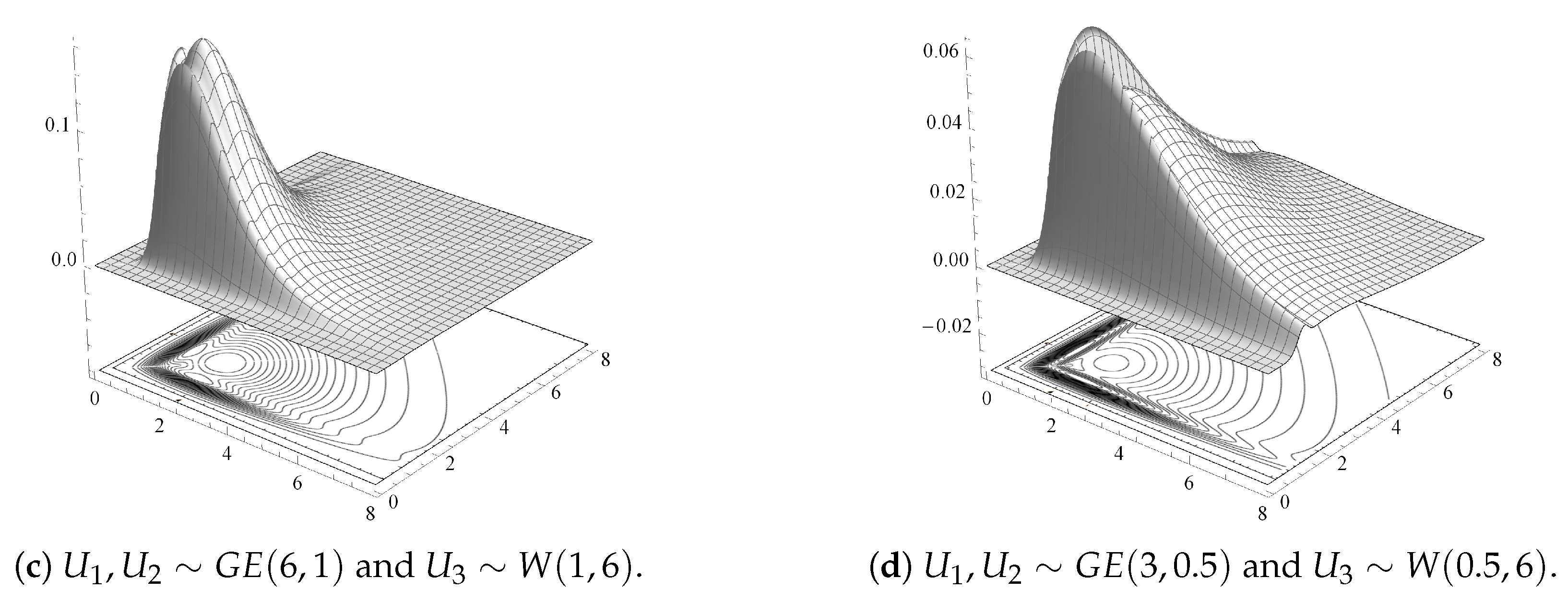
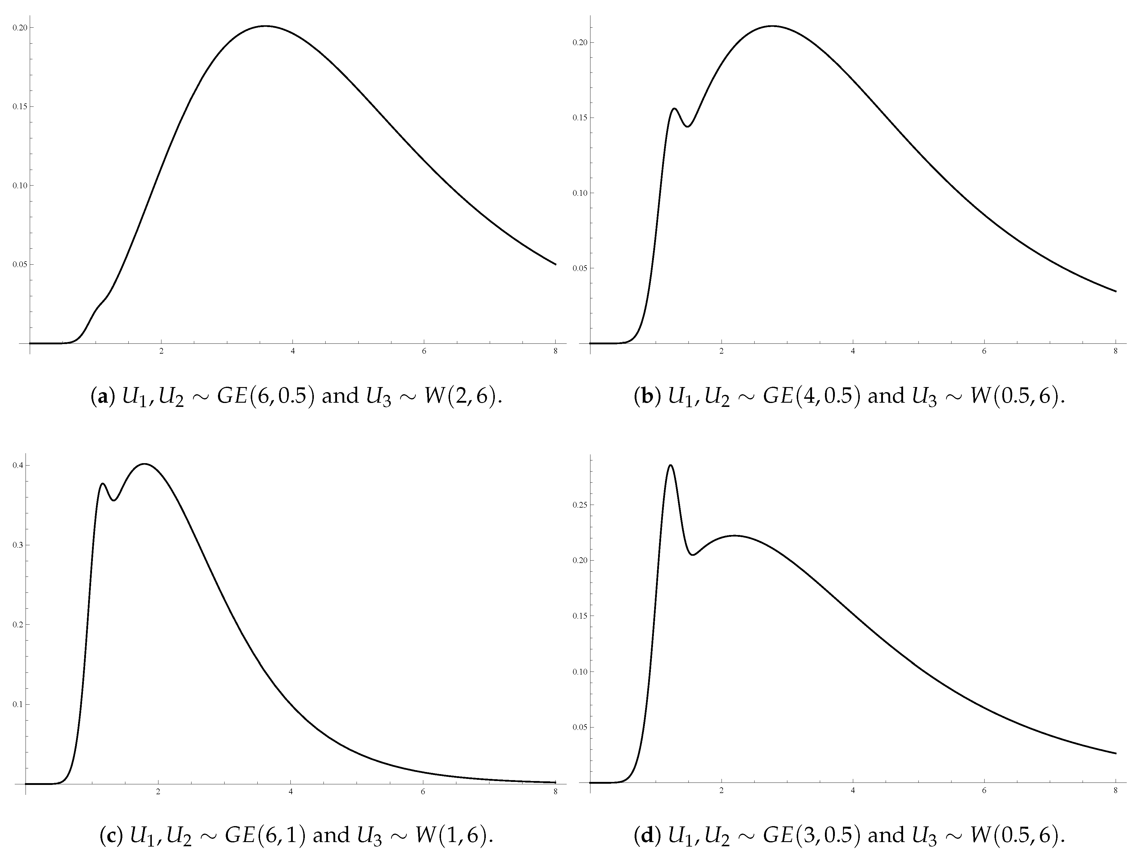
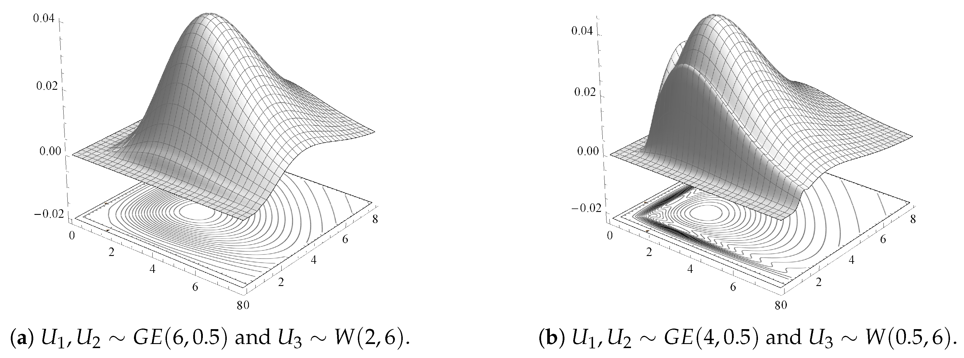
For illustrative purposes, Figure 1a–d display 3D surfaces of different joint pdfs given by Theorem 3, along with their contour plots. Here, $U_1$ and $U_2$ are taken identically distributed $GE(\theta ,\lambda )$ with different shape and scale parameter values, and $U_3$ having a Weibull distribution with scale parameter ${\lambda }_3$ and shape parameter $\alpha =6$, $W({\lambda }_3,6)$.

Figure 1 shows that some of these GBD models are multi-modal bivariate models. It indicates a variety of shapes for the GBD family depending on the different baseline distribution components and for different parameter values.

4. Distributional Properties

Here, we derive the marginal and conditional distributions of the GBD family, and the order statistics. Furthermore, some properties for particular baseline distribution vectors are provided.

4.1. Marginal and Conditional Distributions

From Theorem 1, it is easy to obtain the marginal cdfs of the components $X_i$’s, which can be written as

$$F_{X_i}\left(x_i\right)=F_{U_i}\left(x_i\right)F_{U_3}\left(x_i\right),\mathrm{with}i=1,2,$$

(5)

and, when the pdf $f_{U_i}$ of $U_i$ exists, $i=1,2,3$, the corresponding pdfs are given by

$$f_{X_i}\left(x_i\right)=f_{U_i}\left(x_i\right)F_{U_3}\left(x_i\right)+F_{U_i}\left(x_i\right)f_{U_3}\left(x_i\right),\mathrm{with}i=1,2.$$

(6)

For instance, we shall now suppose that $U_i$s have PRH distributions, in order to provide some preservation results of the PRH property on the marginals, and its closure under exponentiation of the underlying distributions.

Proposition 1.

If $(X_1,X_2)$ has a GBD model formed by $U_i\sim PRH\left({\theta }_i\right)$ with baseline distribution $F_{B_i}$ ($i=1,2,3$), then $X_i\sim PRH({\theta }_i+{\theta }_3)$ with base distribution $F_{B_i^{*}}=F_{B_i}^{{\theta }_i/({\theta }_i+{\theta }_3)}{F}_{B_3}^{{\theta }_3/({\theta }_i+{\theta }_3)}$. Moreover, when the base distribution is common, $F_B=F_{B_i}$, then $X_i$s also have the same baseline distribution $F_B$.

Proof. 

It immediately follows from (5) and the EBPRH model, since $F_{U_i}=F_{B_i}^{{\theta }_i}$. □

Corollary 1.

If $U_i\sim PRH\left({\theta }_i\right)$ with base distribution $F_{B_i}$, having $F_{B_i}\sim PRH\left({\lambda }_i\right)$ with base distribution $F_{{\tilde{B}}_i}$ ($i=1,2,3$), then $X_i\sim PRH({\theta }_i{\lambda }_i+{\theta }_3{\lambda }_3)$ with base distribution $F_{B_i^{*}}=F_{{\tilde{B}}_i}^{{\theta }_i{\lambda }_i/({\theta }_i{\lambda }_i+{\theta }_3{\lambda }_3)}{F}_{{\tilde{B}}_3}^{{\theta }_3{\lambda }_3/({\theta }_i{\lambda }_i+{\theta }_3{\lambda }_3)}$. Moreover, if $F_{\tilde{B}}=F_{{\tilde{B}}_i}$ ($i=1,2,3$), then $X_i$s also have the same base distribution $F_{\tilde{B}}$.

In addition, Figure 2 displays the plots of the marginal pdfs of the GBD models depicted in Figure 1a–d.

Note that Figure 2a–d show some bimodal shapes for the marginal pdfs given by (6) of the GBD models represented in Figure 1a–d, which also exhibit some multi-modal shapes of the joint pdfs. In this setting, Proposition 1 might be used to generate bimodal distributions from the marginals of the GBD family by mixing different baseline distribution components as in Figure 1.

Furthermore, we provide some results about the conditional distributions of a GBD model whose proof can be found in Appendix A.

Theorem 4.

If $(X_1,X_2)$ has a GBD model with baseline distribution vector $(F_{U_1},F_{U_2},F_{U_3})$, then

1. 

The conditional distribution of $X_i$ given $X_j\le x_j$ ($i\ne j$), say $F_{i|X_j\le x_j}$, is an absolutely continuous cdf given by

$$F_{i|X_j\le x_j}\left(x_i\right)=\left\{\begin{array}{cc}{F}_{U_i}\left(x_i\right)\frac{F_{U_3}\left(x_i\right)}{F_{U_3}\left(x_j\right)},\hfill & if{x}_i<x_j\hfill \\ F_{U_i}\left(x_i\right),\hfill & if{x}_i\ge x_j\hfill \end{array}\right..$$

2. 

The conditional pdf of $X_i$ given $X_j=x_j$ ($i\ne j$), say $f_{i|X_j=x_j}$, is a convex combination of an absolutely continuous cdf and a degenerate cdf given by

$$f_{i|X_j=x_j}\left(x_i\right)={\alpha }_j{I}_{x_j}\left(x_i\right)+(1-{\alpha }_j)f_{i|x_j,ac}\left(x_i\right),$$

where $I_{x_j}$ is the indicator function of the given point $x_j$, and $f_{i|x_j,ac}$ is the absolutely continuous part

$$f_{i|X_j=x_j,ac}\left(x_i\right)=\frac{1}{1-{\alpha }_j}\left\{\begin{array}{cc}{f}_{X_i}\left(x_i\right)\frac{f_{U_j}\left(x_j\right)}{f_{X_j}\left(x_j\right)},\hfill & if{x}_i<x_j\hfill \\ f_{U_i}\left(x_i\right),\hfill & if{x}_i>x_j\hfill \\ 0,\hfill & if{x}_i=x_j\hfill \end{array}\right.$$

and the mixing weight ${\alpha }_j$ is constant with respect to $x_i$

$${\alpha }_j=F_{U_1}\left(x_j\right)F_{U_2}\left(x_j\right)\frac{f_{U_3}\left(x_j\right)}{f_{X_j}\left(x_j\right)}.$$

4.2. Minimum and Maximum Order Statistics

Now, we provide the cdfs of the maximum and minimum order statistics of a GBD model, which may be interpreted as the lifetimes of parallel and series systems based on the components of $(X_1,X_2)$.

Theorem 5.

If $T_1=min(X_1,X_2)$ and $T_2=max(X_1,X_2)$ of a GBD model $(X_1,X_2)$ with baseline distribution vector $(F_{U_1},F_{U_2},F_{U_3})$, then their cdfs are given by

$$F_{T_1}\left(x\right)=F_{U_3}\left(x\right)F_{U_{1:2}}\left(x\right)\mathit{and}{F}_{T_2}\left(x\right)=F_{U_{3:3}}\left(x\right)$$

(7)

where $U_{1:2}=min(U_1,U_2)$ and $U_{3:3}=max(U_1,U_2,U_3)$.

Proof. 

It is trivial from (1) and (5) by taking into account that $F_{T_2}\left(x\right)=F(x,x)$ and $F_{T_1}\left(x\right)=F_{X_1}\left(x\right)+F_{X_2}\left(x\right)-F_{T_2}\left(x\right)$. □

The pdfs $f_{T_1}$ and $f_{T_2}$ of the minimum and maximum statistics can be readily obtained by differentiation of (7).

Furthermore, the PRH property is preserved by the maximum order statistic of a GBD model, which is immediately derived from Theorem 5.

Corollary 2.

If $U_i\sim PRH\left({\theta }_i\right)$ with baseline distribution $F_{B_i}$ ($i=1,2,3$), then $T_2\sim PRH\left(\theta \right)$ with base $F_{B_{\left(2\right)}}=F_{B_1}^{{\theta }_1/\theta }{F}_{B_2}^{{\theta }_2/\theta }{F}_{B_3}^{{\theta }_3/\theta }$ and $\theta ={\theta }_1+{\theta }_2+{\theta }_3$. Moreover, when $F_B=F_{B_i}$ ($i=1,2,3$), then $T_2$ also has the same base distribution $F_B$.

5. Dependence and Stochastic Properties

In this section, we study various dependence and stochastic properties on the GBD family, its marginals and order statistics, and its copula representation. Notions of dependence and ageing for bivariate distributions can be found in Lai and Xie [34] and Balakrishnan and Lai [4]; see also Shaked and Shantikumar [35] for univariate and multivariate stochastic orders.

5.1. GBD Model

Proposition 2.

If $(X_1,X_2)\sim GBD$ model, then $(X_1,X_2)$ is positive quadrant dependent (PQD).

Proof. 

From (1) and (5), it is readily obtainable that $F(x_1,x_2)\ge F_{X_1}\left(x_1\right)F_{X_2}\left(x_2\right)$, which is equivalent to say that all random vector $(X_1,X_2)$, having a GBD model, is PQD. □

An immediate consequence of the PQD property is that $Cov(X_1,X_2)>0$. Other important bivariate dependence properties are the following, whose proofs are provided in Appendix A.

Proposition 3.

Let $(X_1,X_2)$ be a random vector having a GBD model:

1. 

$(X_1,X_2)$ is left tail decreasing (LTD).

2. 

$(X_1,X_2)$ is left corner set decreasing (LCSD).

3. 

Its joint cdf F is totally positive and of order 2 ($T{P}_2$).

Proof. 

Note that F is $T{P}_2$ is equivalent to $(X_1,X_2)$ is LCSD, which implies LTD (e.g., see Balakrishnan and Lai [4]). Thereby, we only have to prove (3). From the definition of $T{P}_2$ property, it is equivalent to check that the following inequality holds:

$$\frac{F\left(\mathit{x}\right)F\left({\mathit{x}}^{\prime }\right)}{F(\mathit{x}\vee {\mathit{x}}^{\prime })F(\mathit{x}\wedge {\mathit{x}}^{\prime })}\le 1,$$

(8)

for all $\mathit{x}$ and ${\mathit{x}}^{\prime }$, where $\mathit{x}\vee {\mathit{x}}^{\prime }=(max(x_1,x_1^{\prime }),max(x_2,x_2^{\prime }))$, and $\mathit{x}\wedge {\mathit{x}}^{\prime }=(min(x_1,x_1^{\prime }),min(x_2,x_2^{\prime }))$. Hence, from (1), the inequality (8) can be expressed as

$$\frac{F_{U_3}\left(u\right)F_{U_3}\left(v\right)}{F_{U_3}\left(w\right)F_{U_3}\left(y\right)}\le 1,$$

where $u=x_1\wedge x_2$, $v=x_1^{\prime }\wedge x_2^{\prime }$, $w=(x_1\vee x_1^{\prime })\wedge (x_2\vee x_2^{\prime })$ and $y=u\wedge v$. Moreover, one can observe that $y\le u\vee v=max(u,v)\le w$.

Therefore, when $u\le v$, i.e., $y=u\le v\le w$, the inequality (8) can be simplified as follows:

$$\frac{F_{U_3}\left(v\right)}{F_{U_3}\left(w\right)}\le 1,$$

which is trivial, since $v\le w$ and $F_{U_3}$ is a cdf. An analogous development follows for $u>v$, which completes the proof. □

Let us see now some results related to the reversed hazard gradient of a random vector from the GBD family, which is defined as an extension of the univariate case, see Domma [36],

$$r\left(\mathit{x}\right)=(r_1\left(\mathit{x}\right),r_2\left(\mathit{x}\right))=\left(\frac{\partial }{\partial x_1},\frac{\partial }{\partial x_2}\right)lnF(x_1,x_2)$$

where each $r_i\left(\mathit{x}\right)$ represents the reversed hazard function of $\left(X_i\right|X_j\le x_j)$, $i\ne j=1,2$, and assuming that F is differentiable. In addition, it is said that $(X_1,X_2)$ has a bivariate decreasing (increasing) reversed hazard gradient, BDRHG (BIRHG), if all components $r_i$s are decreasing (increasing) functions in the corresponding variables.

Proposition 4.

If $(X_1,X_2)$ has a GBD model with baseline distribution vector $(F_{U_1},F_{U_2},F_{U_3})$, then its reversed hazard gradient $r\left(\mathit{x}\right)$ is given by

$$r_i\left(\mathit{x}\right)=\left\{\begin{array}{cc}{r}_{U_i}\left(x_i\right)+r_{U_3}\left(x_i\right),\hfill & if{x}_i<x_j\hfill \\ r_{U_i}\left(x_i\right),\hfill & if{x}_i\ge x_j\hfill \end{array}\right.$$

for $i\ne j=1,2$, when the reversed hazard function of $U_i$, $r_{U_i}=f_{U_i}/F_{U_i}$ exists, $i=1,2,3$.

Proof. 

The proof is straightforward from the definition of reversed hazard rate function corresponding to the conditional cdf $F_{i|X_j\le x_j}$ given by (1) of Theorem 4. □

Theorem 6.

Let $(X_1,X_2)$ be a random vector having a GBD model. If $U_i$s have decreasing reversed hazard functions (DRH), then $(X_1,X_2)\in BDRHG$.

Proof. 

It is straightforward from Proposition 4. □

Note that Theorem 6 provides the closure of the DRH property under the formation of a GBD model. Thus, the bivariate extension of a DRH distribution $F_U$ generated by the GBD family is BDRHG.

Nevertheless, it does not hold for the increasing reversed hazard (IRH) property, since both $r_i\left(\mathit{x}\right)$ given in Proposition 4 have a negative jump discontinuity at $x_i=x_j$ for $i\ne j=1,2$. Therefore, if $U_i\in IRH$, then $(X_1,X_2)$ cannot be BIRHG.

Finally, we present some interesting stochastic ordering results between bivariate random vectors of GBD type.

Theorem 7.

Let $\mathit{X}=(X_1,X_2)$ and $\mathit{Y}=(Y_1,Y_2)$ have GBD models with baseline distribution vectors $(F_{U_1},F_{U_2},F_{U_3})$ and $(F_{V_1},F_{V_2},F_{V_3})$, respectively. If $U_i{\le }_{st}{V}_i$ ($i=1,2,3$), then $\mathit{X}{\le }_{lo}\mathit{Y}$.

Proof. 

The result immediately follows from the stochastic ordering between components and (1), since $U_i{\le }_{st}{V}_i$ is equivalent to $F_{U_i}\left(x\right)\ge F_{V_i}\left(x\right)$, and the lower orthant ordering is defined by the inequality $F_X\left(\mathit{x}\right)\ge F_Y\left(\mathit{x}\right)$ for all $\mathit{x}=(x_1,x_2)$. □

Corollary 3.

Let $\mathit{X}\sim EBPRH(\mathit{\theta },\mathit{\lambda })$ and $\mathit{Y}\sim EBPRH({\mathit{\theta }}^{*},{\mathit{\lambda }}^{*})$ with base distributions $F_{B_i}$ and $F_{B_i^{*}}$ ($i=1,2,3$), respectively. If ${\theta }_i\le {\theta }_i^{*}$ and $F_{B_i}{\le }_{st}{F}_{B_i^{*}}$ ($i=1,2,3$), then $\mathit{X}{\le }_{lo}\mathit{Y}$.

Proof. 

It is obvious that $F_{B_i}^{{\theta }_i}\left(x_i\right)\ge F_{B_i}^{{\theta }_i^{*}}\left(x_i\right)\ge F_{B_i^{*}}^{{\theta }_i^{*}}\left(x_i\right)$, i.e., $U_i{\le }_{st}{V}_i$, and then the proof readily follows from Theorem 7. □

Remark 1.

From Corollary 3, if both EBPRH models are based on a common base distribution vector, $F_{B_i}=F_{B_i^{*}}$ ($i=1,2,3$), then it is only necessary that ${\theta }_i\le {\theta }_i^{*}$ to hold the lower orthant ordering.

5.2. Marginals and Order Statistics

Now, we study some stochastic properties of the marginals and the minimum and maximum order statistics of the GBD model.

Firstly, from (5) and (6), the reversed hazard function of the marginal $X_i$s can be expressed as

$$r_{X_i}\left(x\right)=\frac{f_{X_i}\left(x\right)}{F_{X_i}\left(x\right)}=r_{U_i}\left(x\right)+r_{U_3}\left(x\right),i=1,2.$$

(9)

Therefore, the DRH (IRH) property is preserved to the marginals.

Theorem 8.

If $(X_1,X_2)$ has a GBD model formed by $U_i\in DRH$ ($i=1,2,3$), then $X_i\in DRH$ ($i=1,2$).

Remark 2.

Note that the IRH distributions have upper bounded support [37]. Thus, if any $U_i$ is not upper bounded, its reversed hazard function is always decreasing at the end, and then the marginal cannot be IRH. Therefore, it is necessary that $U_i\in IRH$ ($i=1,2,3$) and they have the same upper bounds to be $X_i\in IRH$ ($i=1,2$).

Example 1.

Suppose $U_i$s have extreme value distributions of type 3 with a common support, $U_i\sim EV3(\beta ,{\lambda }_i,k_i)$, whose cdf is defined by

$$F_{U_i}\left(u\right)=exp\left(-{\lambda }_i{(\beta -u)}^{k_i}\right),\mathit{for}u\le \beta$$

and $F_{U_i}\left(u\right)=1$ otherwise. Its reversed hazard function is given by

$$r_{U_i}\left(u\right)={\lambda }_i{k}_i{(\beta -u)}^{k_i-1},\mathsf{for}u\in (-\infty ,\beta ],$$

which is increasing (decreasing) in its support for $k_i\le (\ge )1$. Thus, if $k_i\le (\ge )1$ ($i=1,2,3$), then $U_i\in IRH\left(DRH\right)$, and, consequently, $X_i\in IRH\left(DRH\right)$ ($i=1,2$).

Example 2.

If $(X_1,X_2)$ has an EBGE model, then its marginals are $DRH$, since $r_{X_i}$ given by (9) is the sum of two decreasing functions because of each $U_i\sim GE({\theta }_i,{\lambda }_i)$ is a $PRH\left({\theta }_i\right)$ with exponential baseline distribution

$$r_{U_i}\left(u\right)={\theta }_i{r}_{Exp\left({\lambda }_i\right)}\left(u\right)=\frac{{\theta }_i{\lambda }_i}{e^{{\lambda }_{i}u}-1},$$

which is evidently a decreasing function. Here, $Exp\left(\lambda \right)$ denotes an exponential random variable with mean $1/\lambda$.

Remark 3.

From (9), when the $U_i$s have a common distribution $F_U$, then the marginals $X_i\sim PRH\left(2\right)$ with base distribution $F_U$. Therefore, $r_{X_i}\left(x\right)=2r_U\left(x\right)$ has the same monotonicity. In particular, if $F_U\in DRH\left(IRH\right)$, then $X_i\in DRH\left(IRH\right)$.

Remark 4.

From (9), if $U_i\sim PRH\left({\theta }_i\right)$ with the same base distribution $F_B$, then $X_i\sim PRH({\theta }_i+{\theta }_3)$ with base $F_B$, i.e., $r_{X_i}\left(x\right)=({\theta }_i+{\theta }_3)r_B\left(x\right)$. Thus, Remark 3 also holds by using $F_B$ instead of $F_U$.

Secondly, the mean inactivity time (MIT), also called mean waiting time [37], of a random variable X is defined as

$$m_X\left(x\right)=E(x-X|X\le x)={\int }_{-\infty }^x\frac{F_X\left(y\right)}{F_X\left(x\right)}dy.$$

Thus, from (5), the MIT of the marginal $X_i$s of a GBD model can be derived by

$$m_{X_i}\left(x\right)=\frac{1}{F_{U_i}\left(x\right)F_{U_3}\left(x\right)}{\int }_{-\infty }^x{F}_{U_i}\left(y\right)F_{U_3}\left(y\right)dy,i=1,2.$$

(10)

Here, we shall focus on two particular cases of GBD models, having baseline components with monotonous MIT, which is preserved by the marginals.

Example 3.

Suppose $U_i\sim Exp\left(\lambda \right)$, then its MIT can be expressed as

$$m_{U_i}\left(u\right)=\frac{u}{1-e^{-\lambda u}}-\frac{1}{\lambda },$$

which is an increasing MIT function (IMIT), i.e., $U_i\in IMIT$. From (10), we obtain the MIT function of the marginals $X_i$s for the bivariate exponential version of GBD type,

$$m_{X_i}\left(x\right)=\frac{(2\lambda x-3+4e^{-\lambda x})-e^{-2\lambda x}}{2\lambda {(1-e^{-\lambda x})}^2}.$$

Then, upon differentiation, $m_{X_i}^{\prime }\left(x\right)$ has the same sign as the expression $1-e^{-2\lambda x}-2\lambda x{e}^{-\lambda x}$, which is positive, and therefore $X_i\in IMIT$ ($i=1,2$).

Example 4.

Suppose $U_i\sim EV3(\beta ,{\lambda }_i,k=2)$, then its MIT can be expressed as

$$m_{U_i}\left(u\right)=\frac{1}{e^{-{\lambda }_i{(\beta -u)}^2}}{\int }_{-\infty }^u{e}^{-{\lambda }_i{(\beta -y)}^2}dy=\frac{\Phi (u;\mu ,{\sigma }_i)}{\varphi (u;\mu ,{\sigma }_i)},\mathrm{for}u\le \beta$$

where $\Phi (u;\mu ,{\sigma }_i)$ and $\varphi (u;\mu ,{\sigma }_i)$ are the cdf and pdf of a normal model with $\mu =\beta$ and ${\sigma }_i=\frac{1}{\sqrt{2{\lambda }_i}}$, respectively. Moreover, taking into account that a random variable and its standardized version have PRH functions, and the standard normal distribution has the DRH property [38], we obtain that $U_i\in IMIT$.

Upon considering the cdf of $U_i$s and (5), the marginal $X_i\sim EV3(\beta ,{\lambda }_i+{\lambda }_3,2)$ ($i=1,2$). Thus, their MIT can be written as

$$m_{X_i}\left(x\right)=\frac{\Phi (x;\mu ,{\tilde{\sigma }}_i)}{\varphi (x;\mu ,{\tilde{\sigma }}_i)},\mathrm{for}x\le \beta$$

where ${\tilde{\sigma }}_i=\frac{1}{\sqrt{2({\lambda }_i+{\lambda }_3)}}$ for $i=1,2$, and, consequently, $X_i\in IMIT.$

On the other hand, the following stochastic orderings among the three baseline components of two GBD models are preserved by their corresponding marginals. The proof immediately follows from the definitions of the stochastic orderings.

Theorem 9.

Let $(X_1,X_2)$ and $(Y_1,Y_2)$ have GBD models with base distribution vectors $(F_{U_1},F_{U_2},F_{U_3})$ and $(F_{V_1},F_{V_2},F_{V_3})$, respectively.

1. 

If $U_i{\le }_{st}{V}_i$ ($i=1,2,3$), then $X_i{\le }_{st}{Y}_i$ ($i=1,2$).

2. 

If $U_i{\le }_{rh}{V}_i$ ($i=1,2,3$), then $X_i{\le }_{rh}{Y}_i$ ($i=1,2$).

Finally, we discuss some stochastic properties of the minimum and maximum order statistics of the GBD family. In this setting, from (7), the reversed hazard function of the maximum statistic $T_2$ of $(X_1,X_2)$ of GBD type is determined by the sum of the reversed hazard rates of the baseline distribution vector:

$$r_{T_2}\left(x\right)=r_{U_1}\left(x\right)+r_{U_2}\left(x\right)+r_{U_3}\left(x\right)$$

(11)

when the pdf $f_{U_i}$ of $U_i$ exists, $i=1,2,3$. Hence, it is immediate the following result.

Theorem 10.

If $U_i\in DRH\left(IRH\right)$ ($i=1,2,3$), then $T_2\in DRH\left(IRH\right)$.

Example 5.

Suppose $U_i\sim EV3(\beta ,{\lambda }_i,k_i)$ ($i=1,2,3$). Then, the reversed hazard function of $T_2$ is given by

$$r_{T_2}\left(x\right)=\sum _{i=1}^3{\lambda }_i{k}_i{(\beta -x)}^{k_i-1},$$

and, therefore, if every $k_i\le (\ge )1$, $i=1,2,3$, then $r_{T_2}$ is increasing (decreasing) in x, i.e., $T_2\in IRH\left(DRH\right)$.

Example 6.

If $U_i\sim GE({\theta }_i,{\lambda }_i)$, then the maximum statistic of the EBGE model is $DRH$, $T_2\in DRH$, since (11) is the sum of three decreasing functions.

Remark 5.

When $U_i$s have a common distribution $F_U$, the GBD model has a maximum statistic whose cdf is $F_U$ cube, and (11) can be written as $r_{T_2}\left(x\right)=3r_U\left(x\right)$. In particular, if $F_U\in DRH\left(IRH\right)$, then $T_2\in DRH\left(IRH\right)$.

Remark 6.

From Corollary 2, if $U_i\sim PRH\left({\theta }_i\right)$ with the same base distribution $F_B$, $T_2\sim PRH\left(\theta \right)$ with base $F_B$ and $\theta ={\theta }_1+{\theta }_2+{\theta }_3$, i.e., $r_{T_2}\left(x\right)=\theta r_B\left(x\right)$. Thus, $T_2\in DRH\left(IRH\right)$ if and only if $F_B\in DRH\left(IRH\right)$.

Furthermore, the MIT of the maximum statistic of a GBD model $(X_1,X_2)$ can be derived by

$$m_{T_2}\left(x\right)=\frac{1}{F_{U_1}\left(x\right)F_{U_2}\left(x\right)F_{U_3}\left(x\right)}{\int }_{-\infty }^x{F}_{U_1}\left(y\right)F_{U_2}\left(y\right)F_{U_3}\left(y\right)dy,$$

for each specific baseline distribution vector $(F_{U_1},F_{U_2},F_{U_3})$, when the integral exists. For instance, we will consider a particular case, similar to one used in Example 4.

Example 7.

Suppose $(X_1,X_2)$ has a GBD model with $U_i\sim PRH\left({\theta }_i\right)$ and base distributions $F_{B_i}\sim EV3(\beta ,{\lambda }_i,k=2)$ for $i=1,2,3$, then each component $U_i\sim EV3(\beta ,{\theta }_i{\lambda }_i,2)$, and consequently, $U_i\in IMIT$ for $i=1,2,3$. Moreover, from Corollary 2, the maximum statistic $T_2\sim EV3(\beta ,{\theta }^{*},2)$ with ${\theta }^{*}={\theta }_1{\lambda }_1+{\theta }_2{\lambda }_2+{\theta }_3{\lambda }_3$. Thus, $T_2\in IMIT$ which is obtained along the same line as Example 4, since

$$m_{T_2}\left(x\right)=\frac{\Phi (x;\beta ,{\left(2{\theta }^{*}\right)}^{-1/2})}{\varphi (x;\beta ,{\left(2{\theta }^{*}\right)}^{-1/2})},\mathit{for}x\le \beta .$$

Regarding the minimum statistic $T_1$ of $(X_1,X_2)$ of GBD type, some preservation results are also obtained based on its reversed hazard rate $r_{T_1}$, the proofs are given in Appendix A, and from (7) $r_{T_1}$ can be written as

$$r_{T_1}\left(x\right)=r_{U_{1:2}}\left(x\right)+r_{U_3}\left(x\right).$$

(12)

Theorem 11.

If $U_i\in DRH$ ($i=1,2,3$) and $U_{1:2}{\le }_{rh}{U}_i$ ($i=1,2$), then $T_1\in DRH$.

Corollary 4.

If $U_i\in DRH$ ($i=1,2,3$) and $U_1{=}_{st}{U}_2$, then $T_1\in DRH$.

Example 8.

Suppose $U_i\sim GE(\theta ,\lambda )$ for $i=1,2$ and $U_3\sim GE({\theta }_3,{\lambda }_3)$, then $U_i\in DRH$, and, consequently, $T_1\in DRH$ from Corollary 4.

Remark 7.

Note that, when $U_i$s have a common distribution $F_U$, (12) can be expressed as $r_{T_1}\left(x\right)=r_U\left(x\right)(3-2/(2-F_U\left(x\right)))$, and from Corollary 4, it is immediate to have that, if $F_U\in DRH$, then $T_1\in DRH$.

Theorem 12.

Let $(X_1,X_2)$ be a GBD model. Then, $T_1{\le }_{rh}{T}_2$.

Proof. 

From (11) and (12), the statement is equivalent to $r_{U_{1:2}}\left(x\right)\le r_{U_{2:2}}\left(x\right)$, which readily follows from Theorem 1.B.56 of Shaked and Shanthikumar [35], since the baseline components $U_i$s are independent. □

5.3. Copula and Related Association Measures

Let us see now the copula representation of the GBD family and some related dependence measures of interest in the analysis of two-dimensional data.

It is well known that the dependence between the random variables $X_1$ and $X_2$ is completely described by the joint cdf $F(x_1,x_2)$, and it is often represented by a copula which describes the dependence structure in a separate form from the marginal behaviour. In this setting, from Sklar’s theorem (e.g., see [39]), if its marginal cdfs $F_{X_i}$s are absolutely continuous, then the joint cdf has a unique copula representation for

$$F(x_1,x_2)=C\left(F_{X_1}\left(x_1\right),F_{X_2}\left(x_2\right)\right),$$

and reciprocally, if $F_{X_i}^{-1}$ is the inverse function of $F_{X_i}$ ($i=1,2$), then there exists a unique copula C in ${[0,1]}^2$, such that

$$C(u_1,u_2)=F\left(F_{X_1}^{-1}\left(u_1\right),F_{X_2}^{-1}\left(u_2\right)\right).$$

Now, we can derive the copula representation for the joint cdf of the GBD family as a function of its base distribution vector $(F_{U_1},F_{U_2},F_{U_3})$. In order to do this, by using (5), the joint cdf (1) can be expressed as

$$F(x_1,x_2)=F_{X_1}\left(x_1\right)F_{X_2}\left(x_2\right)\frac{F_{U_3}(min(x_1,x_2))}{F_{U_3}\left(x_1\right)F_{U_3}\left(x_2\right)}$$

and taking $u_i=F_{X_i}\left(x_i\right)$, the associated copula for an arbitrary base distribution vector $(F_{U_1},F_{U_2},F_{U_3})$ can be written as

$$C(u_1,u_2)=u_1{u}_2\frac{min(A_1\left(u_1\right),A_2\left(u_2\right))}{A_1\left(u_1\right)A_2\left(u_2\right)},$$

(13)

where

$$A_i\left(u_i\right)=F_{U_3}\left({(F_{U_i}\times F_{U_3})}^{-1}\left(u_i\right)\right),i=1,2,$$

which allows us to give an additional result.

Theorem 13.

Let $\mathit{X}=(X_1,X_2)$ and $\mathit{Y}=(Y_1,Y_2)$ be two GBD models with baseline distribution vectors $(F_{U_1},F_{U_2},F_{U_3})$ and $(F_{V_1},F_{V_2},F_{V_3})$, respectively. If $\mathit{X}$ and $\mathit{Y}$ have the same associated copula and $U_i{\le }_{st}{V}_i$, then $\mathit{X}{\le }_{st}\mathit{Y}$.

Proof. 

It is immediate by using Theorem 6.B.14 of Shaked and Shanthikumar [35] and (5), since $U_i{\le }_{st}{V}_i$ implies $X_i{\le }_{st}{Y}_i$. □

Corollary 5.

Let $\mathit{X}=(X_1,X_2)$ and $\mathbf{Y}=(Y_1,Y_2)$ be two GBD models with common baseline distributions, $F_U$ and $F_V$, respectively. If $U{\le }_{st}V$, then $\mathit{X}{\le }_{st}\mathit{Y}$.

Note that (13) provides a general formula to establish the specific copula upon considering two particular continuous and increasing bijective functions $A_1$ and $A_2$ from $[0,1]$ onto $[0,1]$. Fang and Li [40] analyzed some stochastic orderings for an equivalent copula representation to (13) with interesting applications in network security and insurance. In the last section, we shall use the bivariate copula representation (13) to discuss the multivariate extension of the GBD family.

Furthermore, (13) may be considered a generalization of the Marshall–Olkin copula, as displayed in the following results whose proofs are omitted.

Corollary 6.

If $(X_1,X_2)$ has a GBD model with a common base distribution $F_U$, then the copula representation of its joint cdf is

$$C(u_1,u_2)=min(u_1{u}_2^{1/2},u_1^{1/2}{u}_2).$$

Corollary 7.

If $(X_1,X_2)$ has a GBD model with PRHs baseline distribution vector of the same base $F_B$, i.e., $(X_1,X_2)\sim BPRH({\theta }_1,{\theta }_2,{\theta }_3)$, then the copula representation of its joint cdf is

$$C(u_1,u_2)=min\left(u_1{u}_2^{{\theta }_2/({\theta }_2+{\theta }_3)},u_1^{{\theta }_1/({\theta }_1+{\theta }_3)}{u}_2\right).$$

Some association measures for a bivariate random vector $(X_1,X_2)$ of GBD type can be derived from the dependence structure described by the general expression (13) for each particular pair of continuous and increasing bijective functions $A_1$ and $A_2$ determined by the specific baseline distribution vector. For instance, for the special GBD models given in Corollaries 6 and 7, the measures of dependence namely Kendall’s tau, Spearman’s rho, Blomqvist’s beta, and tail dependence coefficients, see Nelsen [39] among others, can be calculated as follows.

Kendall’s tau. The Kendall’s $\tau$ is defined as the probability of concordance minus the probability of discordance between two pairs of independent and identically distributed random vectors, $(X_1,X_2)$ and $(Y_1,Y_2)$, as follows:

$$\tau =P\left((X_1-Y_1)(X_2-Y_2)>0\right)-P\left((X_1-Y_1)(X_2-Y_2)<0\right),$$

and it can be calculated through its copula representation $C(u_1,u_2)$ by

$$\tau =4E\left(C({\mathcal{U}}_1,{\mathcal{U}}_2)\right)-1=1-4{\int \int }_{{[0,1]}^2}\frac{\partial C(u_1,u_2)}{\partial u_1}\frac{\partial C(u_1,u_2)}{\partial u_2}d{u}_{1}d{u}_2$$

(14)

with ${\mathcal{U}}_i$s uniform $[0,1]$ random variables whose joint cdf is C.

For example, if $(X_1,X_2)$ has a GBD model with a common baseline $F_U$, upon substituting from the copula of Corollary 6 in (14), it is easy to check that Kendall’s $\tau =1/3$.

Analogously, from the copula given in Corollary 7 of the GBD model for $PRH\left({\theta }_i\right)$ components with a common base $F_B$, the Kendall’s $\tau$ coefficient (14) can be written as

$$\tau =\frac{{\theta }_3}{{\theta }_1+{\theta }_2+{\theta }_3}.$$

Spearman’s rho. The Spearman’s $\rho$ coefficient measures the dependence by three pairs of independent and identically distributed random vectors, $(X_1,X_2)$, $(Y_1,Y_2)$ and $(Z_1,Z_2)$. It is defined as

$$\rho =3\left(P((X_1-Y_1)(X_2-Z_2)>0)-P((X_1-Y_1)(X_2-Z_2)<0)\right),$$

which can be computed by its copula representation $C(u_1,u_2)$ by

$$\rho =12E\left({\mathcal{U}}_1{\mathcal{U}}_2\right)-3.$$

(15)

Thus, if there is a common base distribution as in Corollary 6, the Spearman’s $\rho$ coefficient between $X_1$ and $X_2$ is $\rho =3/7$.

In the case of $U_i\sim PRH\left({\theta }_i\right)$ with a common base distribution $F_B$, from (15) and Corollary 7, this association measure is

$$\rho =\frac{3{\theta }_3}{2{\theta }_1+2{\theta }_2+3{\theta }_3}$$

which coincides with one obtained by Kundu et al. [9] for this specific GBD model, $(X_1,X_2)\sim BPRH({\theta }_1,{\theta }_2,{\theta }_3)$. As remarked by Kundu et al. [9] for the BPRH model, both coefficients, $\tau$ and $\rho$, vary between 0 and 1 as ${\theta }_3$ varies from 0 to ∞.

Blomqvist’s Beta. The Blomqvist’s $\beta$ coefficient, also called the medial correlation coefficient, is defined as the probability of concordance minus the probability of discordance between $(X_1,X_2)$ and its median point, say $(m_1,m_2)$, taking the following form:

$$\beta =P\left((X_1-m_1)(X_2-m_2)>0\right)-P\left((X_1-m_1)(X_2-m_2)<0\right)=4F(m_1,m_2)-1,$$

and from the copula of its joint cdf F, it can be expressed as

$$\beta =4C(1/2,1/2)-1.$$

(16)

In the case of Corollary 6, it is immediate that the medial correlation coefficient between $X_1$ and $X_2$ is $\beta =\sqrt{2}-1$ when it follows a GBD model with a common baseline distribution.

In the other case, from Corollary 7, the Blomqvist’s $\beta$ coefficient (16) is also readily obtainable between the marginals of a BPRH model:

$$\beta =\left\{\begin{array}{cc}{2}^{{\theta }_3/({\theta }_2+{\theta }_3)},\hfill & \mathrm{if}{\theta }_1\le {\theta }_2\hfill \\ 2^{{\theta }_3/({\theta }_1+{\theta }_3)},\hfill & \mathrm{if}{\theta }_1>{\theta }_2,\hfill \end{array}\right.$$

which takes values between 0 and 1 as ${\theta }_3$ varies from 0 to ∞.

Tail Dependence. The tail dependence measures the association of extreme events in both directions, the upper (lower) tail dependence ${\lambda }_U$ (${\lambda }_L$) provides an asymptotical association measurement in the upper (lower) quadrant tail of a bivariate random vector, given by (if it exists)

$${\lambda }_U\left({\lambda }_L\right)=\underset{u\to 1^{-}\left(0^{+}\right)}{lim}P\left(X_2>(\le )F_{X_2}^{-1}\left(u\right)|X_1>(\le )F_{X_1}^{-1}\left(u\right)\right).$$

Similar to the above association coefficients, the tail dependence indexes can be calculated from the copula representation $C(u_1,u_2)$ of the joint cdf of $(X_1,X_2)$, as follows:

$${\lambda }_U=2-\underset{u\to 1^{-}}{lim}\frac{1-C(u,u)}{1-u}\mathrm{and}{\lambda }_L=\underset{u\to 0^{+}}{lim}\frac{C(u,u)}{u}.$$

(17)

In particular, if $(X_1,X_2)$ follows a GBD model with a common baseline distribution, upon substituting from the copula of Corollary 6 in (17), it is easy to check that ${\lambda }_L=0$ and ${\lambda }_U=1/2$.

In the case of $U_i\sim PRH\left({\theta }_i\right)$ with the same base, from (17) and Corollary 7, it is clear that the tail dependence indexes of the BPRH model are ${\lambda }_L=0$ and

$${\lambda }_U=\left\{\begin{array}{cc}\frac{{\theta }_3}{{\theta }_2+{\theta }_3},\hfill & \mathrm{if}{\theta }_1\le {\theta }_2\hfill \\ \frac{{\theta }_3}{{\theta }_1+{\theta }_3},\hfill & \mathrm{if}{\theta }_1>{\theta }_2,\hfill \end{array}\right.$$

which takes values between 0 and 1 as ${\theta }_3$ varies from 0 to ∞.

6. Maximum Likelihood Estimation

In this section, we address the problem of computing the maximum likelihood estimations (MLEs) of the unknown parameters based on a random sample. The problem can be formulated as follows. Suppose $\{(x_{1i},x_{2i});i=1,\dots ,n\}$ is a random sample of size n from a GBD model, where it is assumed that, for $j=1,2,3$, $U_j$ has the pdf $f_{U_j}(u;{\mathit{\theta }}_j)$ and ${\mathit{\theta }}_j$ is of dimension $p_j$. The objective is to estimate the unknown parameter vector $\mathit{\theta }=({\mathit{\theta }}_1,{\mathit{\theta }}_2,{\mathit{\theta }}_3)$. We use the following partition of the sample:

$$I_1=\{i:x_{1i}<x_{2i}\},I_2=\{i:x_{1i}>x_{2i}\},I_0=\{i:x_{1i}=x_{2i}=x_i\}.$$

Based on the above observations, the log-likelihood function becomes

$$\ell \left(\mathit{\theta }\right)=\sum _{i\in I_0}ln{f}_0(x_i;\mathit{\theta })+\sum _{i\in I_1}ln{f}_1(x_{1i},x_{2i};\mathit{\theta })+\sum _{i\in I_2}ln{f}_2(x_{1i},x_{2i};\mathit{\theta }),$$

where $f_0(x_i;\mathit{\theta })$, $f_1(x_{1i},x_{2i};\mathit{\theta })$, $f_2(x_{1i},x_{2i};\mathit{\theta })$ have been defined in Theorem 3.

Here, it is difficult to compute the MLEs of the unknown parameter vector $\mathit{\theta }$ by solving a $p_1+p_2+p_3$ optimization problem. To avoid that, we suggest using the EM algorithm, and the basic idea is based on considering a random sample of size n from $(U_1,U_2,U_3)$, instead of the random sample of size n from $(X_1,X_2)$. From the observed sample $\{(x_{1i},x_{2i}\}$, the sample $\{(u_{1i},u_{2i},u_{3i});i=1,\dots ,n\}$ has missing values as shown in

Table 1. Relation between $(x_{1i},x_{2i})$ and $(u_{1i},u_{2i},u_{3i})$.

${\mathit{I}}_{\mathit{k}}$	Ordering of ${\mathit{U}}_{\mathit{j}}$	${\mathit{X}}_1$	${\mathit{X}}_2$	Missing
$I_0$	$u_{1i}<u_{2i}<u_{3i}$	$u_{3i}$	$u_{3i}$	$u_{1i}$, $u_{2i}$
$I_0$	$u_{2i}<u_{1i}<u_{3i}$	$u_{3i}$	$u_{3i}$	$u_{1i}$, $u_{2i}$
$I_1$	$u_{1i}<u_{3i}<u_{2i}$	$u_{3i}$	$u_{2i}$	$u_{1i}$
$I_1$	$u_{3i}<u_{1i}<u_{2i}$	$u_{1i}$	$u_{2i}$	$u_{3i}$
$I_2$	$u_{2i}<u_{3i}<u_{1i}$	$u_{1i}$	$u_{3i}$	$u_{2i}$
$I_2$	$u_{3i}<u_{2i}<u_{1i}$	$u_{2i}$	$u_{1i}$	$u_{3i}$

. It is immediate that the MLEs of ${\mathit{\theta }}_1$, ${\mathit{\theta }}_2$ and ${\mathit{\theta }}_3$ can be obtained by solving the following three optimization problems of dimensions $p_1$, $p_2$ and $p_3$, respectively,

$${\ell }_j\left({\mathit{\theta }}_j\right)=\sum _{i=1}^{n}ln{f}_{U_j}(u_{ji};{\mathit{\theta }}_j);j=1,2,3,$$

which are computationally more tractable.

From Table 1, if, $i\in I_0$, then $u_{3i}$ is known, and $u_{1i}$ and $u_{2i}$ are unknown. Similarly, if $i\in I_1$ ($i\in I_2$), then $u_{2i}$ ($u_{1i}$) and $max\{u_{1i},u_{3i}\}$ ($max\{u_{2i},u_{3i}\}$) are known. Hence, in the E-step of the EM algorithm, the ‘pseudo’ log-likelihood function is formed by replacing the missing $u_{ji}$ by its expected value, $u_{jim}\left(\mathit{\theta }\right)$, for $i=1,\dots ,n$ and $j=1,2,3$:

• If $i\in I_0$, then

  $$u_{jim}\left(\mathit{\theta }\right)=E\left(U_j\right|U_j<x_i)=\frac{1}{F_{U_j}\left(x_i\right)}{\int }_{-\infty }^{x_i}u{f}_{U_j}\left(u\right)du,j=1,2.$$
• If $i\in I_1$ and $j,k\in \{1,3\},j\ne k$, then

  $$\begin{array}{cc}\hfill u_{jim}\left(\mathit{\theta }\right)& =E\left(U_j\right|max\{U_1,U_3\}=x_{1i})\hfill \\ \hfill & =x_{1i}P(U_j>U_k)+P(U_j<U_k)\frac{1}{F_{U_j}\left(x_{1i}\right)}{\int }_{-\infty }^{x_{1i}}u{f}_{U_j}\left(u\right)du\hfill \\ \hfill & =x_{1i}{\int }_{-\infty }^{\infty }{f}_{U_j}\left(u\right)F_{U_k}\left(u\right)du+\frac{1}{F_{U_j}\left(x_{1i}\right)}{\int }_{-\infty }^{\infty }{f}_{U_k}\left(u\right)F_{U_j}\left(u\right)du{\int }_{-\infty }^{x_{1i}}u{f}_{U_j}\left(u\right)du.\hfill \end{array}$$
• If $i\in I_2$ and $j,k\in \{2,3\},j\ne k$, then

  $$\begin{array}{cc}\hfill u_{jim}\left(\mathit{\theta }\right)& =E\left(U_j\right|max\{U_2,U_3\}=x_{2i})\hfill \\ \hfill & =x_{2i}P(U_j>U_k)+P(U_j<U_k)\frac{1}{F_{U_j}\left(x_{2i}\right)}{\int }_{-\infty }^{x_{2i}}u{f}_{U_j}\left(u\right)du\hfill \\ \hfill & =x_{2i}{\int }_{-\infty }^{\infty }{f}_{U_j}\left(u\right)F_{U_k}\left(u\right)du+\frac{1}{F_{U_j}\left(x_{2i}\right)}{\int }_{-\infty }^{\infty }{f}_{U_k}\left(u\right)F_{U_j}\left(u\right)du{\int }_{-\infty }^{x_{2i}}u{f}_{U_j}\left(u\right)du.\hfill \end{array}$$

Therefore, we propose the following EM algorithm to compute the MLEs of $\mathit{\theta }$. Suppose at the k-th iteration of the EM algorithm, the value of $\mathit{\theta }$ is ${\mathit{\theta }}^{\left(k\right)}=({\mathit{\theta }}_1^{\left(k\right)},{\mathit{\theta }}_2^{\left(k\right)},{\mathit{\theta }}_3^{\left(k\right)}$), then the following steps can be used to compute ${\mathit{\theta }}^{(k+1)}$:

E-step

• At the k-th step for $i\in I_0$, obtain the missing $u_{1i}$ and $u_{2i}$ as $u_{1im}\left({\mathit{\theta }}^{\left(k\right)}\right)$ and $u_{2im}\left({\mathit{\theta }}^{\left(k\right)}\right)$, respectively. For $i\in I_1$ obtain the missing $u_{1i}$ and $u_{3i}$ as $u_{1im}\left({\mathit{\theta }}^{\left(k\right)}\right)$ and $u_{3im}\left({\mathit{\theta }}^{\left(k\right)}\right)$, respectively. Similarly, for $i\in I_2$, obtain the missing $u_{2i}$ and $u_{3i}$ as $u_{2im}\left({\mathit{\theta }}^{\left(k\right)}\right)$ and $u_{3im}\left({\mathit{\theta }}^{\left(k\right)}\right)$, respectively.
• Form the ’pseudo’ log-likelihood function as ${\ell }_s^{\left(k\right)}\left(\mathit{\theta }\right)={\ell }_{1s}^{\left(k\right)}\left({\mathit{\theta }}_1\right)+{\ell }_{2s}^{\left(k\right)}\left({\mathit{\theta }}_2\right)+{\ell }_{3s}^{\left(k\right)}\left({\mathit{\theta }}_3\right)$, where

  $$\begin{array}{cc}\hfill {\ell }_{1s}^{\left(k\right)}\left({\mathit{\theta }}_1\right)& =\sum _{i\in I_0}ln{f}_{U_1}(u_{1im}\left({\mathit{\theta }}^{\left(k\right)}\right);{\mathit{\theta }}_1)+\sum _{i\in I_1}ln{f}_{U_1}(u_{1im}\left({\mathit{\theta }}^{\left(k\right)}\right);{\mathit{\theta }}_1)+\sum _{i\in I_2}ln{f}_{U_1}(u_{1i};{\mathit{\theta }}_1)\hfill \\ \hfill {\ell }_{2s}^{\left(k\right)}\left({\mathit{\theta }}_2\right)& =\sum _{i\in I_0}ln{f}_{U_2}(u_{2im}\left({\mathit{\theta }}^{\left(k\right)}\right);{\mathit{\theta }}_2)+\sum _{i\in I_1}ln{f}_{U_2}(u_{2i};{\mathit{\theta }}_2)+\sum _{i\in I_2}ln{f}_{U_2}(u_{2im}\left({\mathit{\theta }}^{\left(k\right)}\right);{\mathit{\theta }}_2)\hfill \\ \hfill {\ell }_{3s}^{\left(k\right)}\left({\mathit{\theta }}_3\right)& =\sum _{i\in I_0}ln{f}_{U_3}(u_{3i};{\mathit{\theta }}_3)+\sum _{i\in I_1}ln{f}_{U_3}(u_{3im}\left({\mathit{\theta }}^{\left(k\right)}\right);{\mathit{\theta }}_3)+\sum _{i\in I_2}ln{f}_{U_3}(u_{3im}\left({\mathit{\theta }}^{\left(k\right)}\right);{\mathit{\theta }}_3).\hfill \end{array}$$

M-step

• ${\mathit{\theta }}^{(k+1)}=({\mathit{\theta }}_1^{(k+1)},{\mathit{\theta }}_2^{(k+1)},{\mathit{\theta }}_3^{(k+1)})$ can be obtained by maximizing ${\ell }_{1s}^{\left(k\right)}\left({\mathit{\theta }}_1\right)$, ${\ell }_{2s}^{\left(k\right)}\left({\mathit{\theta }}_2\right)$ and ${\ell }_{3s}^{\left(k\right)}\left({\mathit{\theta }}_3\right)$ with respect to ${\mathit{\theta }}_1$, ${\mathit{\theta }}_2$ and ${\mathit{\theta }}_3$, respectively.

Mainly for illustrative purposes, two particular GBD models will be applied in the next section to show the usefulness of the above EM algorithm. Firstly, we shall consider a GBD model with baseline components having the same distribution type and different underlying parameters. Secondly, we shall use a GBD model with baseline components from different distribution families. The technical details of both of them can be found in Appendix B.

7. Data Analysis

In this section, we present the analysis of two-dimensional data sets in order to show how the proposed EM algorithm can be applied to fit particular GBD models. For that, we shall suppose the following two models described in Appendix B: Model I is the GBD model with the exponential baseline distributions and different underlying parameters, $U_j\sim Exp\left({\lambda }_j\right)$ ($j=1,2,3$). Model II is the GBD model with baseline components from Weibull and generalized exponential distributions, $U_1\sim W({\lambda }_1,{\alpha }_1)$, $U_2\sim W({\lambda }_2,{\alpha }_2)$ and $U_3\sim GE({\alpha }_3,{\lambda }_3)$.

7.1. Soccer Data

We have analyzed a UEFA Champion’s League data set [41], played during the seasons 2004–2005 and 2005–2006. This set represents the soccer data where at least one goal has been scored by a kick goal (penalty kick, foul kick or any other direct kick) by any team and one goal has been scored by the home team. Here, in the bivariate data, $(X_1,X_2)$, $X_1$ represents the time in minutes of the first kick goal and $X_2$ represents the time in minutes scored by the home team. Clearly, all possibilities exist in the data set, namely $X_1<X_2$, $X_1>X_2$ and $X_1=X_2$.

Meintanis [41] analyzed this data set using the Marshall–Olkin bivariate exponential model. The marginals of the Marshall–Olkin bivariate exponential distribution are exponential, and then they have constant hazard functions. A preliminary data analysis indicated that the empirical hazard function of both the marginals are increasing and their reversed hazard functions are decreasing. Hence, it may not be proper to use the Marshall–Olkin bivariate exponential model to analyze this data.

Example 9.

In order to use Model I, we have started the initial guess as ${\lambda }_1^{\left(0\right)}={\lambda }_2^{\left(0\right)}={\lambda }_3^{\left(0\right)}=1$. The algorithm stops after eight iterations, the final estimates and the associated 95% confidence intervals are ${\widehat{\lambda }}_1=0.03126(\pm 0.01121)$, ${\widehat{\lambda }}_2=0.04630(\pm 0.01563)$ and ${\widehat{\lambda }}_3=0.04269(\pm 0.01875)$, with $-257.8871$ being the pseudo log-likelihood value. To check whether it has converged to the maximum or not, the performance of the EM algorithm may be compared with the experimental results obtained by using a quasi-Newton method for solving constrained nonlinear optimization problem, which have been summarized in Appendix C as well as the corresponding ones to the subsequent examples.

One natural question is whether Model I fits the bivariate data or not. We have computed the Kolmogorov–Smirnov (KS) distances with the corresponding p-values between the empirical and fitted cdfs for the marginals and the maximum order statistic. The results are reported in

Table 2. Goodness-of-fit results for UEFA Champion’s League data.

GBD Model	KS (p-Value)
	${\mathit{X}}_1$	${\mathit{X}}_2$	$max\{{\mathit{X}}_1,{\mathit{X}}_2\}$	AIC	BIC
Model I	0.1491 (0.3830)	0.1099 (0.7622)	0.1530 (0.3517)	604.8663	609.6990
Model II	0.0976 (0.8719)	0.0839 (0.9565)	0.1139 (0.7228)	708.5430	718.2085

, and, from them, we cannot reject the null hypothesis that this data are coming from the GBD model with exponential baseline distributions.

Example 10.

Let us consider now Model II. We have started the EM algorithm with the initial guesses as ${\alpha }_1^{\left(0\right)}={\alpha }_2^{\left(0\right)}={\alpha }_3^{\left(0\right)}=1$, ${\lambda }_1^{\left(0\right)}=0.03$, ${\lambda }_2^{\left(0\right)}=0.05$ and ${\lambda }_3^{\left(0\right)}=0.04$. The algorithm converges in nineteen iterations, the final estimates and the associated 95% confidence intervals are ${\widehat{\alpha }}_1=1.2987(\pm 0.3124)$, ${\widehat{\lambda }}_1=0.0097(\pm 0.0005)$, ${\widehat{\alpha }}_2=0.8047(\pm 0.2823)$, ${\widehat{\lambda }}_2=0.0093(\pm 0.0021)$, ${\widehat{\alpha }}_3=1.0037(\pm 0.2879)$, ${\widehat{\lambda }}_3=0.0369(\pm 0.008)$, with $-201.1141$ being the pseudo log-likelihood value.

The KS distances with the corresponding p-values for the marginals and the maximum statistic are reported in Table 2. Thus, based on the p-values, we can say that the GBD model with two baseline Weibull distributions and the third GE one fits the data reasonably well.

Summarizing, it is clear that both of the GBD models provide a good fit to the given data set and the EM algorithm also works quite effectively in both the cases. Now, to compare Models I and II of Examples 9 and 10, which provide a better fit, we compute the Akaike’s information criterion (AIC) and Bayesian information criterion (BIC) values and they are also presented in Table 2. Therefore, based on the AIC and BIC values, it is clear that Model I provides a better fit than Model II to the UEFA Champion’s League data set.

7.2. Diabetic Retinopathy Data

Let us consider now the diabetic retinopathy data set [42], available in the R package “SurvCor” [43]. Such data were investigated by the National Eye Institute to assess the effect of laser photocoagulation in delaying the onset of severe visual loss such as blindness in 197 patients with diabetic retinopathy. For each patient, one eye was randomly selected for laser photocoagulation and the other was given no treatment, being used as the control. The times to blindness in both eyes were recorded in months and the censoring was caused by death, dropout, or the end of the study.

For illustrative purposes, we have considered those patients for which complete data are available. Here, $X_1$ denotes the time to the blindness of the untreated or control eye and $X_2$ denotes the time to blindness of the treated eye. Out of 197 patients, we have complete information of $X_1$ and $X_2$ for 38 patients.

Example 11.

As in Example 9, we have used Model I to analyze the data set. In this case, we have also used the same initial guess as ${\lambda }_1^{\left(0\right)}={\lambda }_2^{\left(0\right)}={\lambda }_3^{\left(0\right)}=1$. We have used the proposed EM algorithm, the iteration stops after 14 iterations, and the estimates of unknown parameters and the corresponding 95% confidence intervals are ${\widehat{\lambda }}_1=0.0653(\pm 0.0175)$, ${\widehat{\lambda }}_2=0.0737(\pm 0.0210)$ and ${\widehat{\lambda }}_3=0.1345(\pm 0.3879)$, with $-172.2314$ being the associated pseudo log-likelihood value.

The KS distances with the corresponding p-values between the empirical and fitted cdfs for the marginals and the maximum statistic are presented in

Table 3. Goodness-of-fit results for diabetic retinopathy data.

GBD Model	KS (p-Value)
	${\mathit{X}}_1$	${\mathit{X}}_2$	$max\{{\mathit{X}}_1,{\mathit{X}}_2\}$	AIC	BIC
Model I	0.1033 (0.8244)	0.1848 (0.1598)	0.1229 (0.6310)	585.9757	590.8884
Model II	0.0920 (0.8960)	0.0952 (0.8706)	0.1152 (0.6778)	592.1515	601.9770

.

Example 12.

As in Example 10, we have analyzed the data set by using Model II. We have started the EM algorithm with the initial guesses ${\alpha }_1^{\left(0\right)}={\alpha }_2^{\left(0\right)}={\alpha }_3^{\left(0\right)}=1$, ${\lambda }_1^{\left(0\right)}=0.06$, ${\lambda }_2^{\left(0\right)}=0.07$ and ${\lambda }_3^{\left(0\right)}=0.13$. The algorithm stops after 27 iterations, the final estimates and the corresponding 95% confidence intervals are ${\widehat{\alpha }}_1=1.0937(\pm 0.2563)$, ${\widehat{\lambda }}_1=0.0447(\pm 0.0146)$, ${\widehat{\alpha }}_2=0.5851(\pm 0.1345)$, ${\widehat{\lambda }}_2=0.2369(\pm 0.0763)$, ${\widehat{\alpha }}_3=0.8995(\pm 0.2787)$, ${\widehat{\lambda }}_3=0.1898(\pm 0.0478)$, with $-125.4519$ being the associated pseudo log-likelihood value.

The KS distances with the corresponding p-values for the marginals and the maximum order statistic are presented in Table 3.

From Table 3, we can also say that the estimated GBD models fit the diabetic retinopathy data reasonably well in both the cases. Moreover, we also present the AIC and BIC values of the two models in Table 3. Therefore, based on the AIC and BIC values, it is clear that Model I provides a better fit than Model II for the diabetic retinopathy data.

8. Discussion and Conclusions

In this paper, we have presented the generalized bivariate distribution family by a generator system based on the maximization process from any three-dimensional baseline continuous distribution vector with independent components, providing bivariate models with dependence structure.

For the proposed GBD family, several distributional and stochastic properties have been established. The preservation of the PRH property for the marginals and the maximum order statistic has been obtained. The positive dependence has been shown between both marginals of the GBD models, some results about stochastic orders and on the preservation of the monotonicity of the reversed hazard function and of the mean inactivity time. Furthermore, the copula representation of the GBD model has been discussed, providing a general formula, and some related dependence measures have been also calculated for specific copulas of particular bivariate distributions of the GBD family. In addition, new bivariate distributions can be generated by combining independent baseline components from different distribution families, and several bivariate distributions given in the literature are derived as particular cases of the GBD family.

Note that, even in the simple case, the MLEs cannot be obtained in explicit forms, and it is required solving a multidimensional nonlinear optimization problem. We have proposed using an EM algorithm to compute the MLEs of the unknown parameters, and it is observed that the proposed EM algorithm perform quite satisfactorily in the two data analyses by using two different models of the GBD family. The experimental results summarized in

Table A1. Summary of fitted GBD models for the two real data. EM rows are the parameters estimated with the EM algorithm for maximizing the pseudo log-likelihood function, along with the log-likelihood, AIC and BIC values, and BFGS rows correspond to the results obtained by applying the Broyden–Fletcher–Goldfarb–Shanno algorithm for maximizing the log-likelihood function.

GBD Model	$\mathit{\theta }$						$\mathit{\ell }\left(\mathit{\theta }\right)$	AIC	BIC
	${\mathit{\alpha }}_1$	${\mathit{\lambda }}_1$	${\mathit{\alpha }}_2$	${\mathit{\lambda }}_2$	${\mathit{\alpha }}_3$	${\mathit{\lambda }}_3$
Soccer data
Model I
EM		0.03126		0.04630		0.04269	−299.4331	604.8663	609.6990
BFGS		0.03116		0.04636		0.04283	−299.4328	604.8656	609.6984
Model II
EM	1.2987	0.0097	0.8047	0.0093	1.0037	0.0369	−348.2715	708.5430	718.2085
BFGS	1.3808	0.00698	0.5652	0.25469	1.53813	0.05219	−295.3057	602.6114	612.2770
Diabetic retinopathy data
Model I
EM		0.0653		0.0737		0.1345	−289.9878	585.9757	590.8884
BFGS		0.06290		0.07181		0.14282	−289.9144	585.8288	590.7415
Model II
EM	1.0937	0.0447	0.5851	0.2369	0.8995	0.1898	−290.0758	592.1515	601.9770
BFGS	1.1477	0.03920	0.7917	0.13923	0.41913	0.08272	−285.5795	583.1590	592.9846

disclose such efficiency of the EM algorithm with respect to a conventional numerical iterative procedure of the Newton-type. In more detail, Table A1 presents the experimental results obtained by the Broyden–Fletcher–Goldfarb–Shanno algorithm for maximizing the log-likelihood function, available in the R package “maxLik” [44].

It is worth mentioning that the bivariate copula representation (13) allows us to discuss its multivariate extension. Let $U_i$s for $i=1,\cdots ,q+1$ be a set of $q+1$ mutually independent random variables with any continuous distribution functions, denoting by $F_{U_i}$ the cdf of each $U_i$. Similarly to (1), the joint cdf of the q-dimensional random vector $(X_1,\cdots ,X_q)$ with $X_i=max(X_1,X_2)$ is given by

$$F(x_1,...x_q)=F_{U_{q+1}}(min(x_1,\cdots ,x_q))\prod _{i=1}^q{F}_{U_i}\left(x_i\right)$$

which can be considered as a generator of q-dimensional distribution models, called generalized multivariate distribution (GMD) family with baseline distribution vector $(F_{U_1},...,F_{U_{q+1}})$. Hence, the q-dimensional copula representation of this GMD family can be expressed as

$$C(u_1,...,u_q)=\left(\prod _{i=1}^q{u}_i\right)\frac{{min}_{i=1,...,q}{A}_i\left(u_i\right)}{{\prod }_{i=1}^q{A}_i\left(u_i\right)},$$

where

$$A_i\left(u_i\right)=F_{U_{q+1}}\left({(F_{U_i}\times F_{U_{q+1}})}^{-1}\left(u_i\right)\right),\mathrm{for}i=1,...,q.$$

From these q-dimensional joint cdf and copula, many distributional and stochastic properties established for the GBD family are extensible to the GMD family. Furthermore, by using this generator of multivariate distributions, the special bivariate models given in Section 3 can be easily extended to the multivariate case, which contain multivariate versions of bivariate distributions given in the literature.