Article

Multi-Stage Change Point Detection with Copula Conditional Distribution with PCA and Functional PCA

1
Division of Science and Mathematics, University of Minnesota-Morris, Morris, MN 56267, USA
2
Business School, Zhengzhou University, Zhengzhou 450001, China
*
Author to whom correspondence should be addressed.
Mathematics 2020, 8(10), 1777; https://doi.org/10.3390/math8101777
Submission received: 28 September 2020 / Revised: 9 October 2020 / Accepted: 9 October 2020 / Published: 14 October 2020

Abstract

:
A global uncertainty environment, such as the COVID-19 pandemic, has affected the manufacturing industry severely in terms of supply and demand balancing. So, it is common that one stage statistical process control (SPC) chart affects the next-stage SPC chart. It is our research objective to consider a conditional case for the multi-stage multivariate change point detection (CPD) model for highly correlated multivariate data via copula conditional distributions with principal component analysis (PCA) and functional PCA (FPCA). First of all, we review the current available multivariate CPD models, which are the energy test-based control chart (ETCC) and the nonparametric multivariate change point model (NPMVCP). We extend the current available CPD models to the conditional multi-stage multivariate CPD model via copula conditional distributions with PCA for linear normal multivariate data and FPCA for nonlinear non-normal multivariate data.

1. Introduction

Since Hotelling (1949) proposed Hotelling T 2 statistics for the multivariate statistical process control (SPC), Crosier (1988), Lowry, Woodall, Champ and Rigdon (1992), and Zou and Tsung (2011) have proposed the multivariate versions of the cumulative sum (CUSUM) time-weighted control chart and the exponentially weighted moving average (EWMA) time-weighted SPCs. However, the manufacturing industry is still requiring a modern statistical technique dealing with non-normal high dimensional correlated multivariate data. In order to solve this difficult problem in lights of quality control, [1] proposed SPC charts as a tool for analyzing big data. Furthermore, Reference [2] discussed and compared the conventional SPCs with nonparametric SPCs in terms of the strengths and limitations.
The purpose of our paper is that, under a situation, such as high dimensional correlated variables over the several stage process in a manufacturing industry business, we consider modeling conditional multi-stage manufacturing processes for detecting faults in the several stages for the complex production system. Multi-stage CPD has emerged as a cutting-edge research area at the interface of the engineering and statistical sciences. Over the last two decades, Reference [3,4,5] developed the change point detection (CPD) models with needed pre-knowledge for in-control distribution and nonparametric CPD charts to detect mean, variance, and other distributional shifts. Reference [6] proposed online nonparametric multivariate CPD models. Recently, Reference [7] reviewed previous works focusing on energy divergence test theory and its applications in the CPD. Reference [8] proposed nonparametric multiple change point analysis of multivariate data which used the energy test for applications, such as a sliding window scheme with fixed window size, to detect change points in image data or a change point retrospective analysis. Reference [9,10] developed the ‘ecp’ R package for nonparametric multiple change point analysis of multivariate data. Reference [7] also proposed a nonparametric control chart for detecting multiple change points from multivariate time series, which is energy test-based control chart (ETCC), and compared their method with another nonparametric control chart, called nonparametric multivariate change point (NPMVCP), which was developed by [6]. The advantage of using ETCC by Reference [7] is that ETCC detects the changepoints of the mean and covariance together. Reference [11] also reviewed multi-stage manufacturing processes, and Reference [12] reviewed recent research in a dynamic screening system for sequential process monitoring. In this paper, we want to extend the current available multivariate CPD models into the conditional multi-stage multivariate CPD model via copula conditional distribution. Recently, copula modeling has been popular in biostatistics, economics, and finance because copula functions do not need normal, linear, and independent assumptions. Furthermore, copula approaches to quality control for monitoring the bivariate auto-correlated binary observations have been discussed by Reference [13,14] because copulas do not require any assumptions, such as independence, linearity, and normality, for the residual analysis, and it is possible to look at both the marginal distributions and the joint dependence structure [15].
The layout of the paper is as follows. Section 2 describes principal component analysis (PCA), functional PCA (FPCA), copula definitions, ETCC, and NPMVCP, and Section 3 describes our conditional multi-stage multivariate CPD procedure. Section 4 illustrates our proposed method with a simulated multivariate data and the real exchange currency data in America, Asia, and Europe. Finally, conclusions and future research studies are presented in Section 5.

2. Statistical Methods

We consider a situation, such as high dimensional correlated variables over conditional multi-stage processes. Among several statistical methods for the dimensional reduction of multivariate highly correlated variables, we employ the traditional linear PCA and a nonlinear FPCA in this paper. With the traditional PCA method, we consider normal multivariate data for the conditional multi-stage CPD. With a nonlinear FPCA method, we consider non-normal multivariate data for the conditional multi-stage CPD. For extending single-stage CPD to the conditional multi-stage CPD, we employ the conditional distribution by copula and the nonparametric multivariate control chart for the conditional multi-stage CPD.

2.1. Principal Component Analysis

The traditional linear PCA is one of the popular statistical methods to reduce the dimensionality of multivariate data into a smaller number of uncorrelated variables called principal components (PCs), while keeping variation in the original data.
The SPCs with primary principal components by PCA have been proposed to monitor a class of multivariate quality processes for handling multivariate data with multicollinearity between variables (see Reference [16] for details). We consider the PCA-based multivariate CPD method to demonstrate the model’s flexibility and performance by both a simulation study and a real data illustration based on Reference [7]. If the data follows the normality assumption, then we can use our proposed conditional multi-stage CPD with a linear PCA method.

2.2. Functional Principal Component Analysis

For the dimension reduction of the multivariate highly correlated and non-normal data, we also employ nonlinear FPCA to determine the factors (i.e., principal components). By using non-liner eigenfunctions to explain the variation of the time series and examine the sample covariance structure, FPCA is a better statistical dimension reduction method than the PCA proposed by Reference [17]. In addition, FPCA is the more appropriate statistical method to know the clustering pattern of the time-course data rather than the clustering pattern of the whole data at a certain time. We divide density variations into a set of orthogonal principal component functions that maximize the variance along each component estimating density functions by employing a nonparametric method and extracting common structures from the estimated functions.
The functional form of y i ( t ) is given by the sum of the weighted basis functions, ϕ k ( t ) , across the set of times T.
y i ( t ) = Σ k = 1 K c i k ϕ k ( t ) ,
where K is a number of basis functions. In this study, a Fourier basis is used to represent smooth functions as a basis function due to its flexibility and computational advantages. Here, our goal is to obtain a smooth function which fits well into the observed time series, y i ( t ) . To perform FPCA, we use the ‘fdapace’ R package (Reference [18]). This package is FPCA for sparsely or densely sampled random trajectories and time courses, via the principal analysis by conditional estimation (PACE) algorithm which produces covariance and mean functions, eigenfunctions, and principal component (scores), for both functional data and derivatives for both dense (functional) and sparse (longitudinal) sampling designs. For sparse designs, PACE gives fitted continuous trajectories with confidence bands, even for subjects with few longitudinal observations. Reference [19,20] developed the basic procedure behind the PACE approach for sparse functional data as follows: First, compute the cross-sectional mean μ ^ . Second, compute the cross-sectional covariance surface which is guaranteed to be positive semi-definite. Third, do eigenanalysis on the covariance to estimate the eigenfunctions ϕ ^ and eigenvalues λ ^ . Fourth, employ numerical integration to estimate the corresponding scores η ^ , i.e., η i k ^ = 0 T [ y ( t ) μ ^ ( t ) ] ϕ i ( t ) d t .

2.3. Copula

A copula is defined as a multivariate distribution function defined on the unit [ 0 , 1 ] p , with p the number of marginal distributions. Copula is a flexible function to construct the dependence structure of random variables. In this paper, we consider a bivariate (two-dimensional) copula, where p = 2 . Reference [21] proposed copula function such that any bivariate distribution function, F X Y ( x , y ) , can be represented as a function of its marginal distribution of X and Y, F X ( x ) and F Y ( y ) , as
F X Y ( x , y ) = P ( X x , Y y ) = C ( F X ( x ) , F Y ( y ) , θ ) = C ( U , V , θ ) ,
where we denote U = F X ( x ) and V = F Y ( y ) , which are the continuous cumulative distribution functions of X and Y, and we denote as θ an association parameter of the copula function. Therefore, the copula function describes the dependent mechanism between two random variables by eliminating the influence of the marginal distributions or any monotone transformation of the marginal distributions.
Definition 1.
A p-dimensional copula is a function C : [ 0 , 1 ] p [ 0 , 1 ] with the following properties:
1.
For all ( U 1 , , U p ) [ 0 , 1 ] p , then C ( U 1 , , U p , θ ) = 0 if at least one coordinate of ( U 1 , , U p ) is 0;
2.
C ( 1 , , 1 , U i , 1 , , 1 , θ ) = U i , for all U i [ 0 , 1 ] , ( i = 1 , , p ) ;
3.
C is r-increasing, (see Reference [22]).
Definition 2.
A Gaussian copula is a distribution over [ 0 , 1 ] p . It is constructed from a multivariate normal distribution over R p by using the probability integral transform. For a given correlation matrix R [ 1 , 1 ] p × p , the Gaussian copula with parameter matrix R can be written as
C ( U 1 , , U p , θ ) = Φ R ( Φ 1 ( U 1 ) , , Φ 1 ( U p ) ) ,
where θ is an association parameter of the Gaussian copula function, Φ 1 is the inverse cumulative distribution function of a standard normal, and Φ R is the joint cumulative distribution function of a multivariate normal distribution with mean vector zero and a covariance matrix equal to the correlation matrix R .
Definition 3.
The p-dimensional random vector X = ( X 1 , , X p ) is said to have a (non-singular) multivariate Student-t distribution with ν degrees of freedom, mean vector μ and positive-definite dispersion or scatter matrix Σ, denoted X ~ t p ( ν , μ , Σ ) , if its density is given by
f ( x ) = Γ ν + p 2 Γ ν 2 ( π ν ) p | Σ | 1 + ( x μ ) Σ 1 ( x μ ) ν ν + p 2 .
Note that, in this standard parameterization, c o v ( X ) = ν ν 2 Σ so that the covariance matrix is not equal to Σ and is in fact only defined if ν > 2 . Useful reference for the multivariate t-copula is Reference [23].
Definition 4.
(Archimedean Copula). Let C be an associative, Archimededean copula. Then, there exists a strictly decreasing and convex (hence continuous) function (called the generator) φ : [ 0 , 1 ] [ 0 , + ) with φ ( 1 ) = 0 such that for every pair ( U , V ) in [ 0 , 1 ] × [ 0 , 1 ] ,
C ( U , V , θ ) = φ [ 1 ] ( φ ( U ) + φ ( V ) ) ,
where φ [ 1 ] is the “pseudo-inverse" of φ, given by
φ [ 1 ] ( x ) = φ 1 ( x ) , i f   0 x φ ( 0 ) 0 , i f   φ ( 0 ) < x + .
Table 1 shows the most commonly used Archimedean copula functions, such as Clayton copula, Farlie-Gumbel-Morgenstern (FGM) copula, Frank copula, and Gumbel copula with an association parameter θ of each copula function.
Because of the limited range of the association parameter, θ , in the Clayton copula, FGM copula, and Gumbel copula functions in Table 1, we have difficulty applying the Clayton copula, FGM copula, and Gumbel copula functions to SPC, except for the Frank copula. We employed the Gaussian copula in Definition 1, the t-copula in Definition 2, and one of the Archimedean copula, the Frank copula introduced in Definition 3, for our proposed conditional multi-stage CPD.

2.4. Energy Test-Based Control Chart (ETCC)

Reference [7] proposed a nonparametric CPD model which can simultaneously detect any change of mean, variance, or dependence structure all together in the multivariate distribution. Furthermore, Reference [7] used the maximum energy divergence-based permutation test to screen out the multiple change points for multivariate time series and employs the discrepancy of empirical characteristic functions of two random vectors. The empirical distribution of the test statistic can be obtained by permutation samples. Then, the sequential detection of change points can be performed under the algorithm introduced by the change point model (see Reference [24]) to form an online detection. For a change point detection problem, it is set that the change occurs at τ when the two random vectors { X i R p : X i ~ F , i = 1 , , τ } and { Y j R p : Y j ~ G , j = τ + 1 , , T } have a distribution shift. In a multiple change point case, τ i , i = 1 , 2 , , the changes’ detection can be formulated as
X t ~ F 0 , t τ 1 F 1 , τ 1 < t τ 2 F 2 , τ 2 < t τ 3 F j , τ j < t τ j + 1 .
Because the corresponding characteristic functions of X i and Y j , i.e., f x and f y , are uniquely determined, using the divergence between characteristic functions of the two random vectors to monitor the change is an applicable routine. Reference [25] employed an integrated weighted distance between two characteristic functions, and proved that the larger the distance, the more likely a change may occur between the two random vectors. Reference [7] named a nonparametric CPD model which is a nonparametric control chart as an energy test-based control chart (ETCC). Based on the ETCC, Reference [26] made an R package ‘EnergyOnlineCPM’ which centers on the Phase II nonparametric CPD model to online detect the multiple change points.

2.5. NPMVCP by Holland and Hawkins (2014)

Reference [6] proposed a nonparmatric SPC by employing multivariate rank-based test by Reference [27]. The multivariate CPD model by Reference [24] defines changes in a sequence, X 1 , , X t , as follows:
X i ~ F ( μ ) , i τ F ( μ + σ ) , i > τ ,
and H 0 : σ = 0 , versus H 1 : σ 0 . The test statistics and their asymptotic distribution are given for k { 1 , , t 1 } as:
t k t k r ¯ t ( k ) T Σ ˜ k , t 1 r ¯ t ( k ) d χ d 2 ,   i f   t ,
where Σ ˜ k , t is the pooled sample covariance matrix for the centered rank vector r ¯ t ( k ) computed by using a kernel function. Reference [6] developed the test statistic
r k , t = r ¯ t ( k ) T Σ ^ k , t 1 r ¯ t ( k ) ,
where Σ ^ k , t = t k t k Σ ^ t is the unpooled estimator of the covariance matrix of the centered ranks.

3. Multi-Stage CPD with Copula Conditional Distribution

In this research, we consider the conditional multi-stage multivariate CPD by performing the conditional transformed data by copula functions (Gaussian, t, Frank).
Corollary 1.
For two random variables X 1 and X 2 , we can derive the conditional distribution of X 1 given X 2 , F 1 | 2 ( X 1 | X 2 ) , as follows:
F 1 | 2 ( X 1 | X 2 ) = C ( U 1 , U 2 , θ 12 ) U 2 ,
where θ 12 is an association parameter of the copula function, U 1 = F ( X 1 ) , and U 2 = F ( X 2 ) . Similarly, for two random variables X 2 and X 3 , we can derive the conditional distribution of X 3 given X 2 , F 3 | 2 ( X 3 | X 2 ) , as follows:
F 3 | 2 ( X 3 | X 2 ) = C ( U 2 , U 3 , θ 23 ) U 2 ,
where θ 23 is an association parameter of the copula function, U 2 = F ( X 2 ) , and U 3 = F ( X 3 ) .
Corollary 2.
Assume we have three random variables X 1 , X 2 , X 3 . We can derive the conditional cumulative distribution function as follows:
F 3 | 12 ( X 3 | X 1 , X 2 ) = C ( U 1 , U 2 , U 3 , θ 3 | 12 ) U 1 U 2 ,
where θ 3 | 12 is an association parameter of the copula function, U 1 = F ( X 1 ) , U 2 = F ( X 2 ) , and U 3 = F ( X 3 ) .
The procedures for estimating the parameter of the copula for the conditional distribution function can be defined as follows. The first step is that we employ the empirical CDF approach to transform the observations to uniform distributed data in [0, 1]. (see Reference [28] for details). Because the empirical marginal distributions of U and V are uniform on [ 0 , 1 ] such that they are parameter-free, the rank-based approach allows us to compute joint probabilities without knowing marginal distributions. In this paper, the association parameter estimation for bivariate copulas is computed by using a maximum likelihood estimation method which can be used in the ‘BiCopEst’ function from the ‘CDVine’ R package [29]. The second step is that after the parameters θ i j and θ j k in C ( U i , U j , θ i j ) and C ( U j , U k , θ j k ) are estimated, the conditional CDFs C ( U i , U j , θ ^ i j ) U j = F ( X i | X j ) = U i | j and C ( U j , U k , θ ^ j k ) U j = F ( X k | X j ) = U k | j are computed with the estimates θ ^ i j and θ ^ j k by partial derivatives of C ( U i , U j , θ ^ i j ) and C ( U j , U k , θ ^ j k ) . The third step is that the association parameter θ i k | j of C ( F ( X i | X j ) , F ( X k | X j ) , θ i k | j ) = C ( U i | j , U k | j , θ i k | j ) is estimated by the maximum likelihood estimation method. The last step is that with the estimated parameter θ ^ i k | j , the conditional CDF C ( U i | j , U k | j , θ ^ i k | j ) U i | j = F ( X k | X i , X j ) = U k | i j is computed. By following these procedures, we can make the conditional transformed data with a copula function for conditional multi-stage CPD.
For the dimensional reduction to the smaller number of principal components compared to the number of variables in the whole dataset, we apply PCA or FPCA to each stage dataset ( X i , i = 1 , 2 , 3 ), and, iteratively, we perform PCA or FPCA on each stage dataset( X i , i = 1 , 2 , 3 ) to do a dimensional reduction. Each stage size is n i for i = 1 , 2 , 3 , and we set an equal sample size for each stage ( n 1 = n 2 = n 3 ) for the computation convenience of the copula method such that n = n 1 + n 2 + n 3 for the simulated multivariate data X = ( X 1 , X 2 , X 3 ) . After performing PCA or FPCA with X = ( X 1 , X 2 , X 3 ) , we transform the PCA scores generated from X = ( X 1 , X 2 , X 3 ) to the uniform distribution transformed data Y = ( Y 1 , Y 2 , Y 3 ) by the empirical CDF approach, and then we apply the copula conditional distribution to these Y = ( Y 1 , Y 2 , Y 3 ) , so that the conditional transformed data are generated, such as the Y 1 vector, F ( Y 2 | Y 1 ) vector, and F ( Y 3 | Y 1 , Y 2 ) vector.
Finally, we employ the energy test-based control chart (ETCC, Reference [7]) and nonparametric multivariate change point model (NPMVCP, Reference [6]) of each stage for detecting change points to the Y 1 vector, F ( Y 2 | Y 1 ) vector, and F ( Y 3 | Y 1 , Y 2 ) vector. We propose the conditional multi-stage CPD scheme based on the copula conditional distributions and PCA or FPCA for multivariate correlated data as follows:
  • Apply PCA or FPCA to the simulated multivariate data X = ( X 1 , X 2 , X 3 ) for dimensional reduction to several principal components.
  • Transform the PCA or FPCA scores to the uniform distribution transformed data Y = ( Y 1 , Y 2 , Y 3 ) by the empirical CDF approach.
  • Apply the copula conditional distribution for transforming three-stage multivariate data Y = ( Y 1 , Y 2 , Y 3 ) to two conditional datasets F ( Y 2 | Y 1 ) and F ( Y 3 | Y 1 , Y 2 ) .
  • Apply multivariate CPD methods (ETCC and NPMVCP) to both conditional stages F ( Y 2 | Y 1 ) and F ( Y 3 | Y 1 , Y 2 ) .
  • Detect change points by ETCC and NPMVCP from each F ( Y 2 | Y 1 ) and F ( Y 3 | Y 1 , Y 2 ) .

4. Illustrated Example

In order to illustrate our proposed conditional multi-stage multivariate CPD, we compare our method with recent multivariate CPD models by using simulated multivariate data and real data in Section 4.

4.1. Simulation Study

We want to generate multi-stage simulated multivariate dataset so that a current stage process is affected by the previous stage process and multivariate data have high correlations among variables, we employed the copula dependence method which can express the multi-stage dependence and can make a high correlation structure among variables in each stage. With this simulated dataset, we want to verify our conditional multi-stage CPD scheme by the copula conditional distribution. We generate three stage simulated datasets ( X 1 , X 2 , X 3 ) . We name X 1 as stage 1, X 2 as stage 2, and X 3 as stage 3.
For the dataset X 1 , we simulate the highly correlated multivariate data by using the ‘copula’ R package with the ‘normalCopula’ function for the five variables, and each variable has sample size 400 with the correlation parameters (0.9, 0.8, 0.8, 0.8, 0.7, 0.7, 0.7, 0.6, 0.5, 0.4), specifying that the type of the symmetric positive definite matrix characterizing the elliptical copula is unstructured. For each marginal distribution for the five variables in X 1 , we use three gamma distributions ( X 11 follows gamma distribution with shape parameter (set to 5) and scale parameter (set to 1), X 12 follows gamma distribution with shape parameter (set to 5) and scale parameter (set to 2), and X 13 follows gamma distribution with shape parameter (set to 5) and scale parameter (set to 3)) and two exponential distributions ( X 14 follows exponential distribution with parameter (set to 5) and X 15 follows exponential distribution with parameter (set to 2)).
For the dataset X 2 , we simulate the highly correlated multivariate data by using ‘copula’ R package with the ‘normalCopula’ function for the five variables, and each variable has sample size 400 with the correlation parameters (0.4, 0.5, 0.6, 0.7, 0.7, 0.7, 0.7, 0.6, 0.5, 0.4), specifying that the type of the symmetric positive definite matrix characterizing the elliptical copula is unstructured. For each marginal distribution for the five variables in X 2 , we use three gamma distributions ( X 21 follows gamma distribution with shape parameter (set to 2) and scale parameter (set to 1), X 22 follows gamma distribution with shape parameter (set to 2) and scale parameter (set to 2), and X 23 follows gamma distribution with shape parameter (set to 2) and scale parameter (set to 3)) and two exponential distributions ( X 24 follows exponential distribution with parameter (set to 2), and X 25 follows exponential distribution with parameter (set to 5)).
For the dataset X 3 , we simulate the highly correlated multivariate data by using ‘copula’ R package with ‘normalCopula’ function for the 5 variables and each variable has sample size 400 with the correlation parameters (0.5, 0.5, 0.5, 0.5, 0.5, 0.5, 0.5, 0.5, 0.5, 0.5) to specify the symmetric positive definite matrix characterizing that the elliptical copula is unstructured. For each marginal distribution for five variables in X 3 , we use three gamma distributions ( X 31 follows gamma distribution with shape parameter (set to 3) and scale parameter (set to 1), X 32 follows gamma distribution with shape parameter (set to 3) and scale parameter (set to 2), and X 33 follows gamma distribution with shape parameter (set to 3) and scale parameter (set to 3)) and two exponential distributions ( X 34 follows exponential distribution with parameter (set to 4), and X 35 follows exponential distribution with parameter (set to 3)).
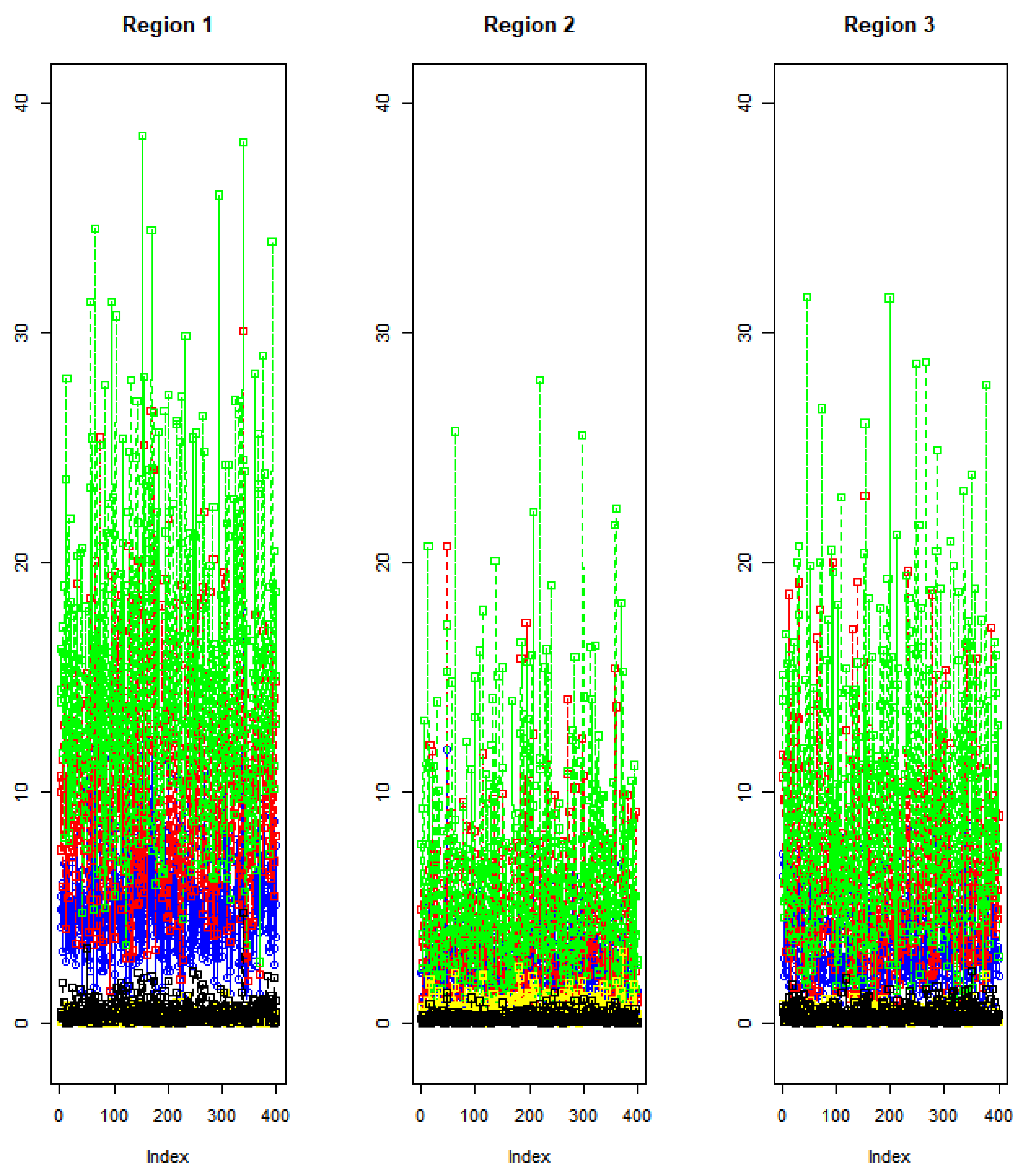
Figure 1 shows the data plots of the three stages ( X 1 , X 2 , X 3 ) . In Figure 1, stage 1 shows bigger spread than stage 2 and stage 3, stage 2 shows smaller spread than stage 1 and stage 3, and stage 3 has bigger spread than stage 2. The correlation matrix with the simulated multivariate data in Table 2 shows high correlations exist among the five variables in X 1 , X 2 , and X 3 .
To perform the change point detection for the conditional multi-stage multivariate highly correlated simulated dataset, we apply PCA or FPCA to the simulated data X = ( X 1 , X 2 , X 3 ) and then generate PCA or FPCA scores to the uniform distribution transformed data Y = ( Y 1 , Y 2 , Y 3 ) by the empirical CDF approach. For FPCA, we employ Fourier basis functions for constructing functional eigenfunctions with K = 7 and T = 433 introduced in Section 2.2, and three eigenfunctions by the FPCA are transformed to the uniform distributed data Y = ( Y 1 , Y 2 , Y 3 ) by the empirical CDF approach. We apply the copula conditional distribution for transforming three-stage multivariate data Y = ( Y 1 , Y 2 , Y 3 ) to two conditional datasets F ( Y 2 | Y 1 ) and F ( Y 3 | Y 1 , Y 2 ) and then apply multivariate CPD methods (ETCC and NPMVCP) to each Y 1 , F ( Y 2 | Y 1 ) and F ( Y 3 | Y 1 , Y 2 ) to detect change points for each stage Y 1 , F ( Y 2 | Y 1 ) and F ( Y 3 | Y 1 , Y 2 ) .
Table 3 shows the PCA variance proportions for X 1 , X 2 and X 3 . Table 4 shows the PCA variance proportions with copula conditional distributions of t-copula, Gaussian copula and Frank copula, F ( Y 2 | Y 1 ) and F ( Y 3 | Y 1 , Y 2 ) . Table 5 shows the change points by both ETCC and NPMVCP with the whole simulated data case and PCA components of the simulated multivariate data. We compare our proposed method with recent methods on multi-stage change point detection of multivariate data. We chose a nonparametric multiple change point analysis of multivariate data developed by Reference [9,10] with ‘ecp’ R package. Table 6 shows change point detections with nonparametric multiple change point analysis of simulated multivariate data with using the command ‘ks.cp3o_delta’ for the change points estimation by pruned objective via the Kolmogorov–Smirnov statistic, and the window size between segments is 30 in the ‘ecp’ R package. Compared with the results of ETCC and NPMVCP in Table 5, James, Zhang, and Matteson (2019) detected more change points with simulated multivariate data for each stage (stage 1, stage 2, stage 3). Table 7 shows the change point detections by both ETCC and NPMVCP with FPCA components of simulated multivariate data. The ETCC and NPMVCP with FPCA components of simulated multivariate data in Table 7 detected more change points with simulated multivariate data for each stage (stage 1, stage 2, stage 3) than the James, Zhang, and Matteson (2019) nonparametric multiple change point method.
For considering the conditional multivariate data, the change point detections by both ETCC and NPMVCP with a copula conditional distribution of the t-copula, Gaussian copula, and Frank copula with PCA components are proposed in this paper. We notice that the performance of our copula-based method depends on the choice of the copula function. But, as we mentioned in Section 2.3, it is difficult to apply many copula functions to SPC because the range of the association parameter, θ , in the Clayton copula, FGM copula, and Gumbel copula functions in Table 1 is restricted so that we had computation difficulty to apply the Clayton copula, FGM copula, and Gumbel copula functions to SPC. Since the range of the association parameter, θ , from the Gaussian copula and the t-copula is θ ( , ) , and the Frank copula is θ ( , ) \ { 0 } , we can compare these copula functions to simulated multivariate data to choose the copula function properly, which is the critical issue about a copula-based CPD method. Table 8 shows the change point detections by both ETCC and NPMVCP with copula conditional distribution of the t-copula, Gaussian copula, and Frank copula with PCA components. From Table 8, we can notice that the change point detections by the three copula functions (Gaussian copula, t-copula, and Frank copula) are slightly different.
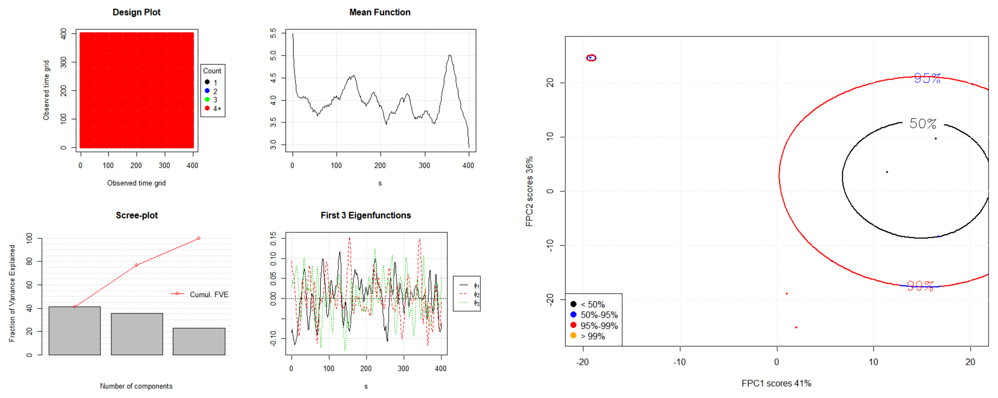
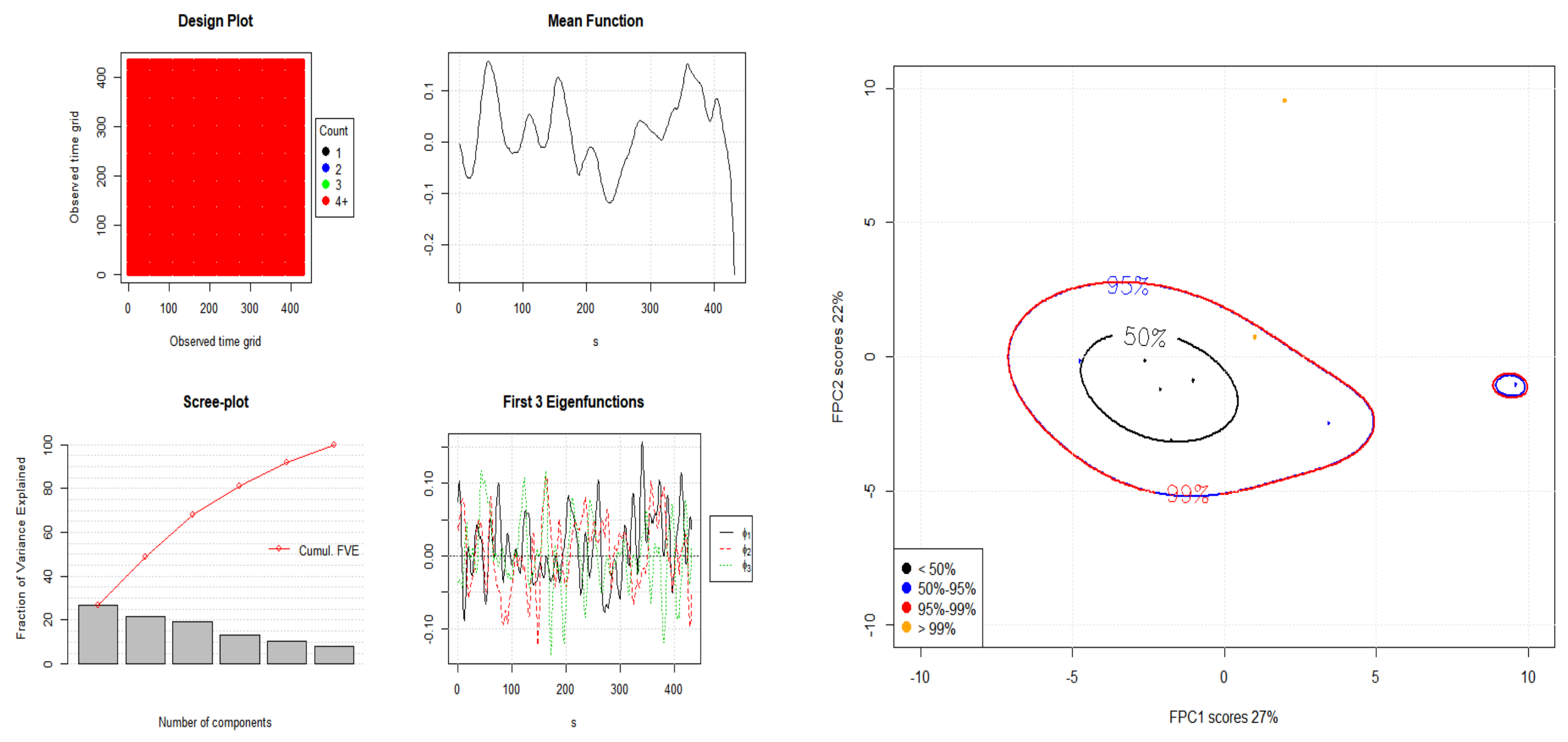
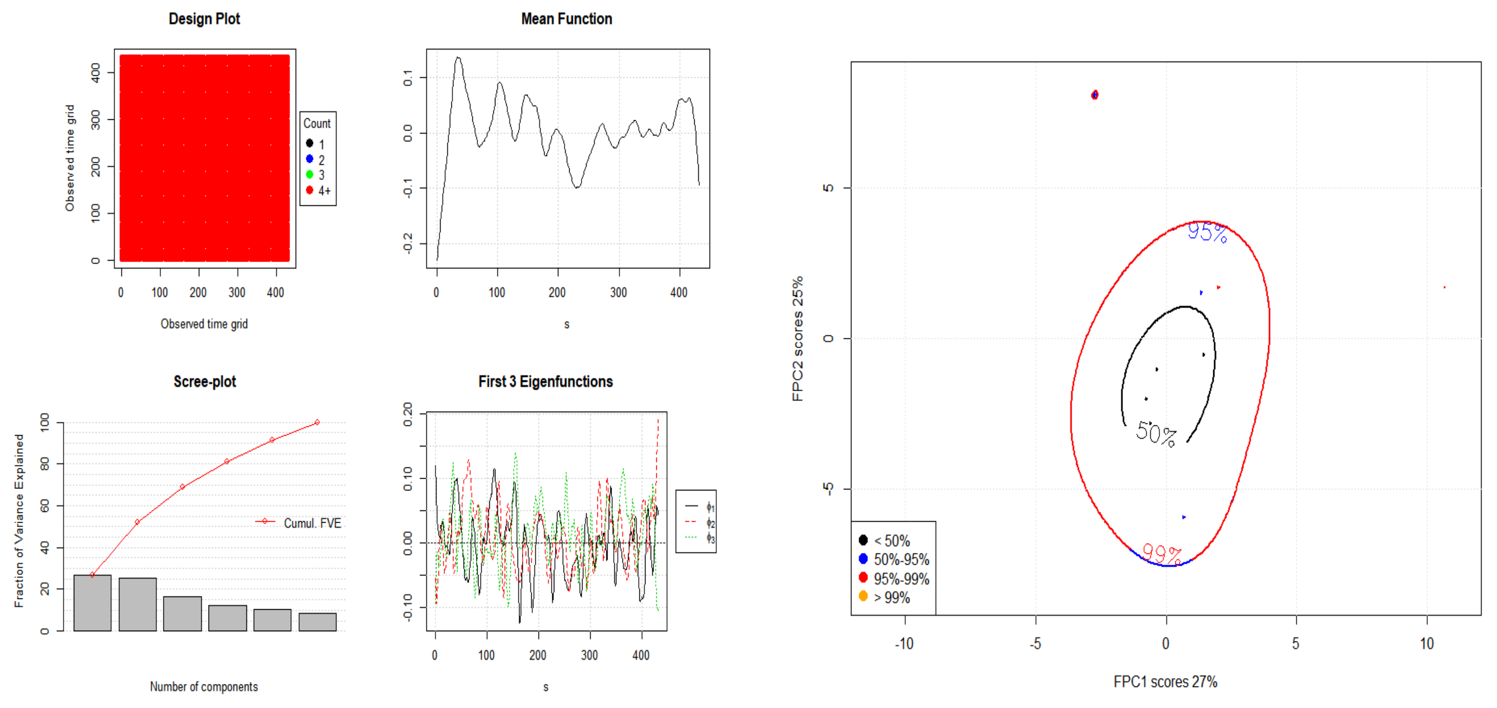
Through the empirical trial and error learning based on the certain manufacturing circumstance, we recommend that industry practitioners compare these copula-based CPD methods and choose a copula function properly. Figure 2, Figure 3 and Figure 4 show the eigenvalues and eigenfunctions of the FPCA plots of X 1 , X 2 , and X 3 . Table 9 shows the change point detections by both ETCC and NPMVCP with a copula conditional distribution of the t-copula, Gaussian copula, and Frank copula with FPCA components. With the simulated multivariate data, we found that the FPCA-based conditional multi-stage multivariate CPD method detected more change points for each stage case rather than the PCA-based conditional multi-stage multivariate CPD method. From Table 9, the FPCA-based conditional multi-stage multivariate CPD method is a promising research area for detecting change points if we can implement the proper copula function empirically.

4.2. Real Data

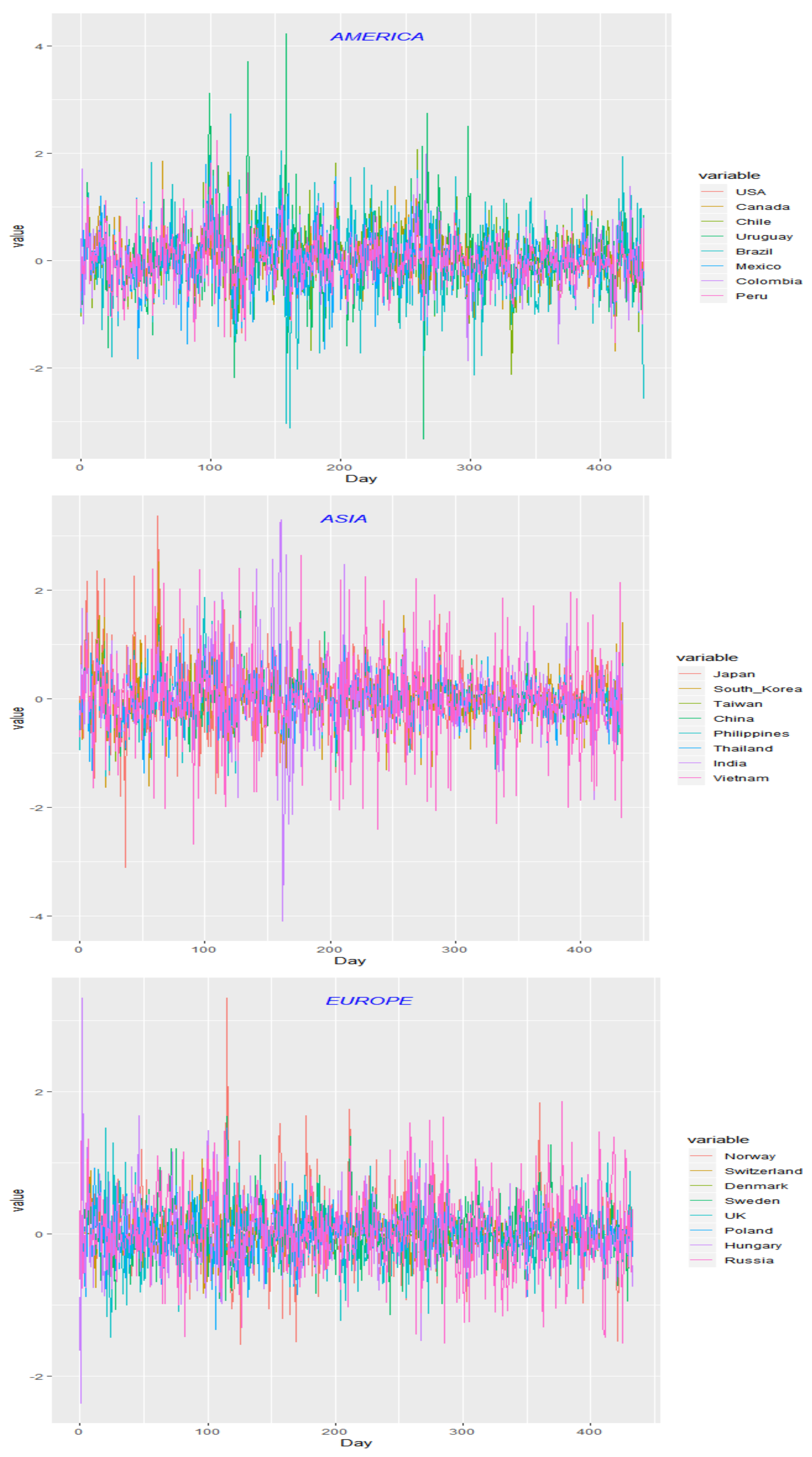
To apply multi-stage multivariate real dataset to our proposed CPD method, we chose daily foreign exchange rates in each continental region which each continental region is financially and economically influenced by another continental region by the time zone difference. Our data set contains daily foreign exchange rates for the twenty four most traded currencies (8 countries in Asia, 8 countries in Europe, and 8 countries in America) against the euro from January 3, 2013 (1/3/2013) to October 6, 2014 (10/6/2014). The data set was retrieved from the currency database retrieval system provided by Professor Werner Antweiler’s website at UBC (University of British Columbia)’s Sauder School of Business, http://fx.sauder.ubc.ca/data.html. We denote S t to be an observed daily foreign exchange rate process in discrete time, t = 1 , , n , and r t = log ( S t / S t 1 ) to be the rates of return of the exchange rates at time t. In particular, we select highest Gross Domestic Product (GDP) to lowest GDP order in each continent so that, in Asia, we select Japan, South Korea, Taiwan, China, Philippines, Thailand, India, and Vietnam; in Europe, we select Norway, Switzerland, Denmark, Sweden, United Kingdom, Poland, Hungary, and Russia; and, in America, we select USA, Canada, Chile, Uruguay, Brazil, Mexico, Columbia, and Peru in Table 10. Figure 5 shows the time plots of the twenty-four currencies in America, Europe, and Asia.
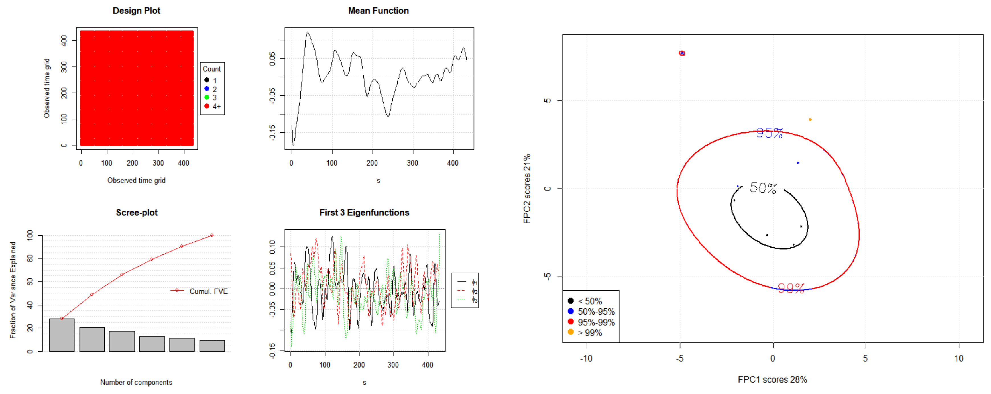
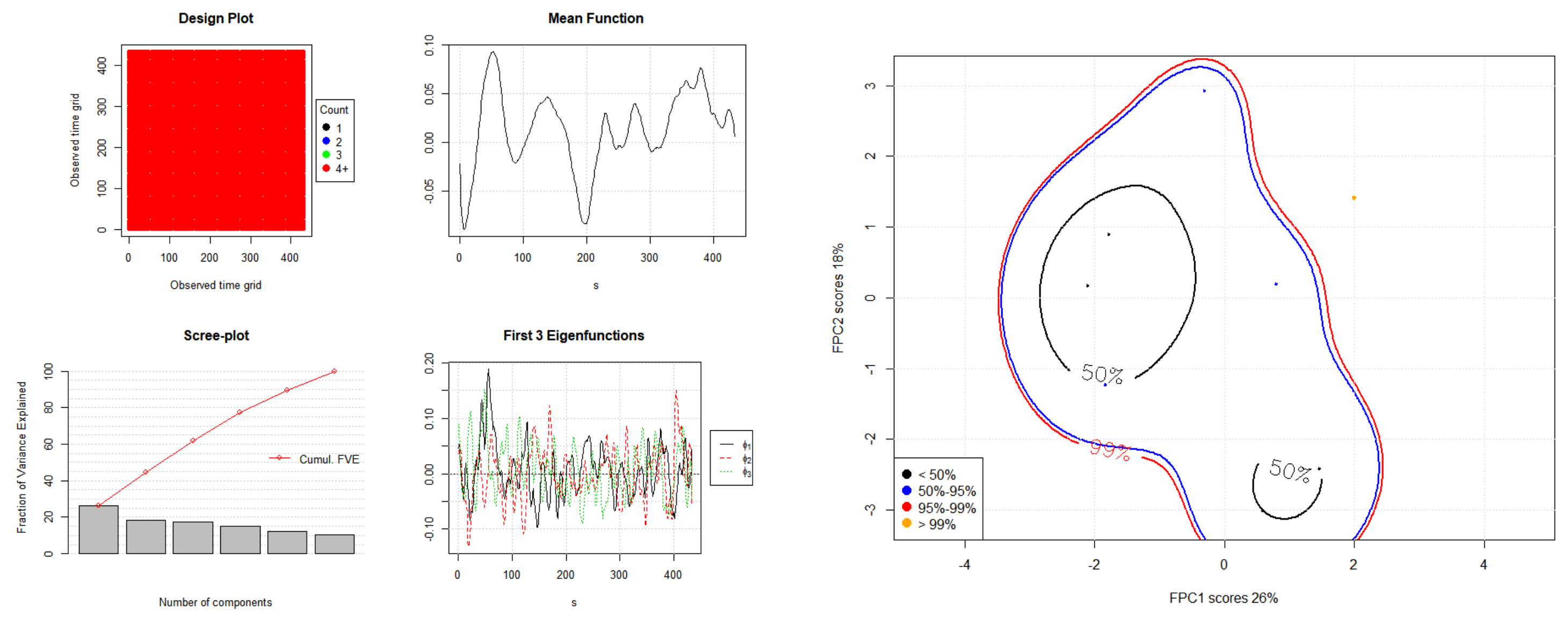
Table 11 shows the correlation matrix with the twenty-four currencies in the period (1/3/2013 to 10/6/2014). We can find that there are high correlations among currencies in Asia and America but not high correlations among currencies in Europe. Table 12 shows the results of PCA variance proportions with real exchange currency data in the period. The result in Table 12 shows that America and Asia have similar PCA component variance proportions but Europe is different from America and Asia in terms of PCA component variance proportions. Table 13 shows PCA variance proportions with copula conditional distributions with t-copula, Gaussian copula, and Frank copula for F(Europe | Asia) and F(America | (Europe, Asia)) of real data. Table 14 shows the change point detection by ETCC and NPMVCP with real exchange currency data and PCA components. Figure 6, Figure 7 and Figure 8 show the eigenvalues and eigenfunctions of FPCA plots of Asia, Europe, and America. Table 15 shows the change points with real exchange currency data by the [9,10] nonparametric multiple change point analysis with the ‘ecp’ R package. Compared with the results of ETCC and NPMVCP in Table 14, Reference [10] detected more change points with real exchange currency data with America, Asia, and Europe (1/3/2013 to 10/6/2014). Table 16 shows change point detections of FPCA components of real exchange currency data with America, Asia, and Europe (1/3/2013 to 10/6/2014). The ETCC and NPMVCP with FPCA components of real data in Table 16 detected more change points with real exchange currency data with America, Asia, and Europe (1/3/2013 to 10/6/2014) than Reference [10] nonparametric multiple change point method. To consider the conditional multivariate real data, the change point detections by ETCC and NPMVCP with copula function of PCA components are shown in Table 17. Table 18 shows change point detection by ETCC and NPMVCP with copula function of FPCA components for real exchange currency data with America, Asia, and Europe (1/3/2013 to 10/6/2014).
For the second real data application, we consider real exchange currency data with America (1/3/2013 to 10/3/2014) and Asia (1/4/2013 to 10/6/2014) because of the time zone difference between America and Asia. Table 19 shows change point detection by ETCC and NPMVCP with real exchange currency data with America (1/3/2013 to 10/3/2014) and Asia (1/4/2013 to 10/6/2014) and the PCA components of the data. Table 20 shows the change point detection with real exchange currency data with America (1/3/2013 to 10/3/2014) and Asia (1/4/2013 to 10/6/2014) by Reference [9,10] nonparametric multiple change point analysis. Compared with the results of ETCC and NPMVCP in Table 19, Reference [10] detected more change points with real exchange currency data with America (1/3/2013 to 10/3/2014) and Asia (1/4/2013 to 10/6/2014). Table 21 shows change point detection by ETCC and NPMVCP with FPCA components of real exchange currency data with America (1/3/2013 to 10/3/2014) and Asia (1/4/2013 to 10/6/2014). The ETCC and NPMVCP with FPCA components of real data in Table 21 detected more change points with real exchange currency data with America (1/3/2013 to 10/3/2014) and Asia (1/4/2013 to 10/6/2014) than [10] nonparametric multiple change point method. We also considered the conditional real data, Asia given America, in terms of time zone difference with America (1/3/2013 to 10/3/2014) and Asia (1/4/2013 to 10/6/2014). Table 22 shows change point detection by ETCC and NPMVCP of the copula conditional distribution and PCA with real exchange currency data of America (1/3/2013 to 10/3/2014) and Asia (1/4/2013 to 10/6/2014). Figure 9 and Figure 10 show the eigenvalues and eigenfunctions of FPCA plots of America (1/3/2013 to 10/3/2014) and Asia (1/4/2013 to 10/6/2014). Table 23 shows change point detection by ETCC and NPMVCP of the copula conditional distribution and FPCA with real exchange currency data of America (1/3/2013 to 10/3/2014) and Asia (1/4/2013 to 10/6/2014). From these two real data examples, we can conclude that the FPCA-based conditional multi-stage multivariate CPD method detected more change points for each stage case rather than the PCA-based conditional multi-stage multivariate CPD method because FPCA is nonlinear PCA, which can be flexible to the real data.
5. Conclusions

We proposed the conditional multi-stage multivariate CPD method by employing PCA or FPCA, copula conditional distribution, and the multivariate CPD models, which are energy test-based control chart (ETCC) and the nonparametric multivariate change point model (NPMVCP). With a simulation study and real data analysis, we showed that our proposed conditional multi-stage multivariate CPD method based PCA and FPCA is useful for detecting change points in the case of a multi-stage sequential process. Furthermore, we can conclude that the FPCA-based conditional multi-stage multivariate CPD method detects more change points compared to the PCA-based conditional multi-stage multivariate CPD method. Future study will employ FPCA with different types of bases to compare Fourier-based FPCA for multi-stage multivariate CPD and also develop a neural network-based multi-stage multivariate CPD method.

Author Contributions

J.-M.K. designed the model, analyzed the data and wrote the paper. N.W. proposed the idea of this paper, formulated the conceptual framework, designed the model, obtained inference and wrote the paper. Y.L. supervised this research, formulated the conceptual framework, designed the model, obtained inference and wrote the paper. All the authors cooperated to revise the paper. All authors have read and agreed to the published version of the manuscript.

Funding

This research was funded by National Natural Science Foundation of China Grant (No. 71672182, No. U1604262 and No. U1904211) and National Social Science Fund of China (No. 20BTJ059).

Conflicts of Interest

The authors declare no conflict of interest.

References

  1. Qiu, P. Statistical process control charts as a tool for analyzing big data. In Big and Complex Data Analysis: Statistical Methodologies and Applications; Ahmem, E., Ed.; Springer: New York, NY, USA, 2017; pp. 123–138. [Google Scholar]
  2. Qiu, P. Some perspectives on nonparametric statistical process control. J. Q. Technol. 2018, 50, 49–65. [Google Scholar] [CrossRef]
  3. Qiu, P.; Hawkins, D. A rank-based multivariate cusum procedure. Technometrics 2001, 43, 120–132. [Google Scholar] [CrossRef]
  4. Qiu, P.; Hawkins, D. A nonparametric multivariate cumulative sum procedure for detecting shifts in all directions. J. R. Stat. Soc. Ser. D Stat. 2003, 52, 151–164. [Google Scholar] [CrossRef]
  5. Ross, G.J.; Tasoulis, D.K.; Adams, N.M. Nonparametric monitoring of data streams for changes in location and scale. Technometrics 2011, 53, 379–389. [Google Scholar] [CrossRef]
  6. Holl, M.; Hawkins, D. A control chart based on a nonparametric multivariate change-point model. J. Q. Technol. 2014, 46, 1975–1987. [Google Scholar] [CrossRef]
  7. Okhrin, O.; Xu, Y.F. A Nonparametric Multivariate Control Chart for High-Dimensional Financial Surveillance. 2017; Submitted under review. [Google Scholar]
  8. Matteson, D.S.; James, N.A. A nonparametric approach for multiple change point analysis of multivariate data. J. Am. Stat. Assoc. 2014, 109, 334–345. [Google Scholar] [CrossRef] [Green Version]
  9. James, N.A.; Matteson, D.S. ecp: An R Package for Nonparametric Multiple Change Point Analysis of Multivariate Data. J. Stat. Softw. 2014, 62, 1–25. [Google Scholar] [CrossRef] [Green Version]
  10. James, N.A.; Zhang, W.; Matteson, D.S. ecp: An R Package for Nonparametric Multiple Change Point Analysis of Multivariate Data. R package, version 3.1.2; 2019. Available online: https://cran.r-project.org/web/packages/ecp/index.html (accessed on 22 August 2019).
  11. Hsu, H.-L.; Ing, C.-K.; Lai, T.L.; Yu, S.-H. Multistage Manufacturing Processes: Innovations in Statistical Modeling and Inference. In Proceedings of the Pacific Rim Statistical Conference for Production Engineering; ICSA Book Series in Statistics; Springer: Singapore, 2018; pp. 67–84. [Google Scholar]
  12. Qiu, P.; You, L. Recent Research in Dynamic Screening System for Sequential Process Monitoring. In Proceedings of the Pacific Rim Statistical Conference for Production Engineering; ICSA Book Series in Statistics; Springer: Singapore, 2018; pp. 85–94. [Google Scholar]
  13. Emura, T.; Long, T.-H.; Sun, L.-H. R routines for performing estimation and statistical process control under copula-based time series models. Commun. Stat. Simul. Comput. 2017, 46, 3067–3087. [Google Scholar] [CrossRef]
  14. Kim, J.-M.; Baik, J.; Reller, M. Control charts of mean and variance using copula Markov SPC and conditional distribution by copula. Commun. Stat. Simul. Comput. 2020. In Press. [Google Scholar] [CrossRef]
  15. Joe, H. Multivariate Models and Multivariate Dependence Concepts; CRC Press: Boca Raton, FL, USA, 1997. [Google Scholar]
  16. Park, K.; Kim, J.-M.; Jung, D. GLM-based statistical control r-charts for dispersed count data with multicollinearity between input variables. Q. Reliab. Eng. Int. 2018, 34, 1103–1109. [Google Scholar] [CrossRef]
  17. Pearson, K. On Lines and Planes of Closest Fit to System of Points in Space. Philos. Mag. 1901, 2, 559–572. [Google Scholar] [CrossRef] [Green Version]
  18. Chen, Y.; Carroll, C.; Dai, X.; Fan, J.; Hadjipantelis, P.Z.; Han, K.; Ji, H.; Lin, S.-C.; Dubey, P.; Mueller, H.-G.; et al. Fdapace: Functional Data Analysis and Empirical Dynamics. R Package. 2019. Available online: https://cran.r-project.org/web/packages/fdapace/index.html (accessed on 17 August 2019).
  19. Liu, B.; Müller, H.-G. Estimating Derivatives for Samples of Sparsely Observed Functions, with Application to Online Auction Dynamics. J. Am. Stat. Assoc. 2009, 104, 704–717. [Google Scholar] [CrossRef]
  20. Yao, F.; Müller, H.-G.; Wang, J.-L. Functional Data Analysis for Sparse Longitudinal Data. J. Am. Stat. Assoc. 2005, 100, 577–590. [Google Scholar] [CrossRef]
  21. Sklar, A. Fonctions de repartition á n dimensions et leurs marges. Publ. Inst. Statist. Univ. Paris 1959, 8, 229–231. [Google Scholar]
  22. Nelsen, R.B. An Introduction to Copulas, 2nd ed.; Springer: Berlin/Heidelberg, Germany, 2013. [Google Scholar]
  23. Demarta, S.; McNeil, A.J. The t copula and related copulas. Int. Stat. Rev. 2005, 73, 111–129. [Google Scholar] [CrossRef]
  24. Hawkins, D.M.; Qiu, P.; Kang, C.W. The changepoint model for statistical process control. J. Q. Technol. 2003, 35, 355–366. [Google Scholar] [CrossRef]
  25. Szekely, G.J.; Rizzo, M.L. Hierarchical clustering via joint between-within distances: Extending Ward’s minimum variance method. J. Classif. 2005, 22, 151–183. [Google Scholar] [CrossRef]
  26. Xu, Y.F. Reference manual: An R package ‘EnergyOnlineCPM’. 2017. Available online: https://sites.google.com/site/EnergyOnlineCPM/ (accessed on 19 March 2020).
  27. Choi, K.; Marden, J. An Approach to Multivariate Rank Tests in Multivariate Analysis of Variance. J. Am. Stat. Assoc. 1997, 92, 1581–1590. [Google Scholar] [CrossRef]
  28. Kim, J.-M.; Hwang, S.Y. Directional Dependence via Gaussian Copula Beta Regression Model with Asymmetric GARCH Marginals. Commun. Stat. Simul. Comput. 2017, 46, 7639–7653. [Google Scholar] [CrossRef]
  29. Brechmann, E.C.; Schepsmeier, U. Modeling Dependence with C- and D-Vine Copulas: The R Package CDVine. J. Stat. Softw. 2013, 52, 1–27. [Google Scholar] [CrossRef] [Green Version]
Figure 1. Plots with simulated multivariate data (region means stage).
Mathematics 08 01777 g001
Figure 2. FPCA Plots of X 1 .
Mathematics 08 01777 g002
Figure 3. FPCA Plots of X 2 .
Mathematics 08 01777 g003
Figure 4. FPCA Plots of X 3 .
Mathematics 08 01777 g004
Figure 5. Twenty-four countries in America, Europe, and Asia (1/3/2013 to 10/6/2014).
Mathematics 08 01777 g005
Figure 6. FPCA plots of Asia (1/3/2013 to 10/6/2014).
Mathematics 08 01777 g006
Figure 7. FPCA lots of Europe (1/3/2013 to 10/6/2014).
Mathematics 08 01777 g007
Figure 8. FPCA plots of America (1/3/2013 to 10/6/2014).
Mathematics 08 01777 g008
Figure 9. FPCA plots of America (1/3/2013 to 10/3/2014).
Mathematics 08 01777 g009
Figure 10. FPCA plots of Asia (1/4/2013 to 10/6/2014).
Mathematics 08 01777 g010
Table 1. Archimedean copula functions.
CopulaCopula Function
FGM C F G M ( U , V , θ ) = U V + θ U V ( 1 U ) ( 1 V ) , θ ( 1 , 1 ]
Clayton C C ( U , V , θ ) = U θ + V θ 1 1 / θ , θ ( 0 , )
Frank C F ( U , V , θ ) = 1 θ log 1 + ( e θ U 1 ) ( e θ V 1 ) e θ 1 , θ R \ { 0 }
Gumbel C G ( U , V , θ ) = exp ( log U ) θ + ( log V ) θ 1 / θ , θ 1
Table 2. Correlation matrix with the simulated multivariate data.Note: X 1 , X 2 and X 3 are vectors.
X 1 X 11 X 12 X 13 X 14 X 15
X 11 10.90050.78730.77620.7778
X 12 0.900510.70810.63990.6988
X 13 0.78730.708110.58580.4561
X 14 0.77620.63990.585810.3780
X 15 0.77780.69880.45610.37801
X 2 X 21 X 22 X 23 X 24 X 25
X 21 10.35010.48430.56440.6425
X 22 0.350110.66260.60100.6890
X 23 0.48430.662610.55590.4614
X 24 0.56440.60100.555910.3409
X 25 0.64250.68900.46140.34091
X 3 X 31 X 32 X 33 X 34 X 35
X 31 10.54090.53250.50970.5043
X 32 0.540910.50070.48430.4783
X 33 0.53250.500710.48110.5467
X 34 0.50970.48430.481110.4540
X 35 0.50430.47830.54670.45401
Table 3. Principal component analysis (PCA) with the simulated multivariate data.
X 1 Comp.1Comp.2Comp.3Comp.4Comp.5
Proportion of Variance0.74620.12290.08410.04090.0059
Cumulative Proportion0.74620.86910.95320.99411.0000
X 2 Comp.1Comp.2Comp.3Comp.4Comp.5
Proportion of Variance0.64870.14940.12020.07070.0111
Cumulative Proportion0.64870.79800.91820.98891.0000
X 3 Comp.1Comp.2Comp.3Comp.4Comp.5
Proportion of Variance0.60990.11570.09810.09120.0851
Cumulative Proportion0.60990.72550.82370.91491.0000
Table 4. PCA variance proportions with simulated multivariate data.
t-CopulaComp.1Comp.2Comp.3
F ( Y 2 | Y 1 ) 0.64870.14940.1202
F ( Y 3 | Y 1 , Y 2 ) 0.60990.11570.0981
Gaussian CopulaComp.1Comp.2Comp.3
F ( Y 2 | Y 1 ) 0.64850.14930.1204
F ( Y 3 | Y 1 , Y 2 ) 0.60990.11550.0982
Frank CopulaComp.1Comp.2Comp.3
F ( Y 2 | Y 1 ) 0.64850.14920.1207
F ( Y 3 | Y 1 , Y 2 ) 0.60950.11530.0985
Table 5. Change point detection by energy test-based control chart (ETCC) and nonparametric multivariate change point (NPMVCP) of PCA with simulated multivariate data.
MethodETCCNPMVCPETCCNPMVCPETCCNPMVCP
X 1 X 2 X 3
Whole data170 191150 186208 264 243 323 368 382193 219 240 304 361 38242 23842 238
PCA Components174174206 218193 218238 296 321238 294 321
Table 6. Change point detection with the James, Zhang, and Matteson (2019) NPMVCP analysis of simulated multivariate data.
Data X 1 X 2 X 3
Change Points85 140 174 241 326 36573 118 160 197 239 318 36150 81 120 155 187 241 279 328
Table 7. Change point detection by ETCC and NPMVCP of functional PCA (FPCA) with simulated multivariate data.
Functional PCA
ETCC
X 1 24 45 68 89 110 131 151 171 191 212 232 252 272 293 313 333 354 375 396
X 2 30 51 71 91 112 133 154 174 194 215 236 257 279 300 320 340 361 382
X 3 21 42 62 82 103 123 144 164 184 208 229 249 269 290 311 332 353 374 397 369 390
NPMVCP
X 1 24 45 68 89 110 130 150 170 191 211 231 251 272 292 312 333 354 375 395
X 2 30 50 70 91 112 133 153 173 194 215 236 257 279 299 319 340 361 381
X 3 21 41 61 82 102 123 143 163 183 208 228 248 269 290 311 332 353 374 397
Table 8. Change point detection by ETCC and NPMVCP of PCA and copulas with simulated multivariate data.
MethodETCCNPMVCPETCCNPMVCP
Copula F ( Y 2 | Y 1 ) F ( Y 3 | Y 1 , Y 2 )
t-Copula212 193 217 369186 192 213 3646 325 327 3315 318 324 331
Gaussian Copula196 209 214 369186 195 213 3646 325 3265 318 324
Frank Copula194 211 215 368186 193 213 36468 296 322 32835 290 316 326
Table 9. Change point detection by ETCC and NPMVCP of FPCA and copulas with simulated multivariate data.
Functional PCA by t-Copula
ETCC
F ( Y 2 | Y 1 ) 11 21 30 38 46 54 61 70 77 85 92 98 102 112 121 131 140 148 156 165 172 181 187 196 200 207
212 219 225 233 241 251 258 266 275 287 294 301 308 313 321 330 337 346 357 365 373 381 390 397
F ( Y 3 | Y 1 , Y 2 ) 11 17 26 32 36 44 49 56 63 70 77 83 88 96 101 109 114 123 129 137 146 151 160 167 175 183 189 197 201
207 216 223 231 239 246 254 265 271 278 286 293 301 308 315 322 330 337 345 353 359 364 372 379 385 394 397
NPMVCP
F ( Y 2 | Y 1 ) 10 20 28 36 45 51 60 69 75 84 90 96 101 110 119 130 138 146 154 162 170 179 185 190 199 205
210 216 224 230 240 249 255 265 274 285 291 300 306 311 320 328 335 345 355 364 370 380 388 395
F ( Y 3 | Y 1 , Y 2 ) 10 15 22 30 35 41 46 55 61 69 75 80 86 94 100 105 113 120 126 136 141 149 159 165 173 181 187 193 199 206
215 221 230 236 244 252 263 270 276 284 290 299 305 314 320 327 335 342 350 357 362 369 375 384 391 396
Functional PCA by Gaussian Copula
ETCC
F ( Y 2 | Y 1 ) 12 21 30 39 48 55 61 71 76 86 96 101 112 120 132 139 147 155 162 172 181 187 192 201 207 213
219 225 232 241 246 253 258 265 275 288 295 302 310 315 320 330 337 346 357 361 367 377 382 390 400
F ( Y 3 | Y 1 , Y 2 ) 14 21 31 41 49 56 65 71 78 81 89 96 101 109 115 123 130 136 146 152 160 168 175 182 189 196 202
209 217 223 232 241 245 255 263 271 278 286 293 300 307 315 323 328 336 345 352 359 363 371 378 385 393
NPMVCP
F ( Y 2 | Y 1 ) 10 20 28 36 45 51 60 69 75 84 95 101 109 119 130 137 145 154 161 170 179 185 190 200 205 210
216 224 230 240 245 251 256 265 274 285 291 300 306 311 319 328 335 345 355 360 366 372 380 388 398
F ( Y 3 | Y 1 , Y 2 ) 12 20 30 40 45 55 61 69 75 80 86 94 100 105 113 120 126 135 140 149 159 165 173 181 187 193 199 206 215 221
230 238 244 253 262 270 276 284 290 298 305 314 320 325 334 341 350 357 362 369 375 384 391
Functional PCA by Frank Copula
ETCC
F ( Y 2 | Y 1 ) 11 22 31 39 43 52 58 63 72 77 85 92 98 102 112 121 130 140 147 156 166 174 181 187 195 201 206
211 217 225 232 241 251 256 266 277 281 286 293 301 308 313 321 331 337 346 356 361 367 375 381 391 400
F ( Y 3 | Y 1 , Y 2 ) 7 16 23 32 41 47 56 64 70 77 83 89 95 103 109 116 122 128 136 142 150 160 167 174 181 188 195 202 209 216
226 231 241 248 255 266 272 278 286 292 300 308 316 323 330 336 344 352 358 363 371 376 386 393
NPMVCP
F ( Y 2 | Y 1 ) 10 20 28 36 41 49 55 61 69 75 84 90 96 101 110 119 129 138 146 154 164 171 179 185 190 200 205 210 216 224
230 240 249 255 265 274 279 285 290 299 305 311 320 328 335 345 355 360 366 372 380 388 398
F ( Y 3 | Y 1 , Y 2 ) 5 14 21 30 40 45 55 61 68 75 80 86 94 100 105 113 120 126 135 140 149 159 165 172 180 187 193 199 206
215 221 230 238 244 252 264 270 276 284 290 299 305 314 320 327 334 341 350 357 362 369 375 384 391
Table 10. Eight countries in Asia, 8 countries in Europe, and 8 countries in America. Order by 2017 GDP.
OrderASIAEUROPEAMERICA
1JAPANNORWAYUSA
2SOUTH KOREASWITZERLANDCANADA
3TAIWANDENMARKCHILE
4CHINASWEDENURUGUAY
5PHILIPPINESUNITED KINGDOMBRAZIL
6THAILANDPOLANDMEXICO
7INDIAHUNGARYCOLUMBIA
8VIETNAMRUSSIAPERU
Table 11. Correlation matrix with real exchange currency data (1/3/2013 to 10/6/2014).
JapanSouth_KoreaTaiwanChinaPhilippinesThailandIndiaVietnam
Japan1.00000.32590.45890.39620.36080.34740.16790.2039
South_Korea0.32591.00000.77890.68450.72090.60150.48520.2849
Taiwan0.45890.77891.00000.87470.79910.72110.49210.3990
China0.39620.68450.87471.00000.74370.69800.45920.4669
Philippines0.36080.72090.79910.74371.00000.69630.56290.3817
Thailand0.34740.60150.72110.69800.69631.00000.51470.3021
India0.16790.48520.49210.45920.56290.51471.00000.2014
Vietnam0.20390.28490.39900.46690.38170.30210.20141.0000
NorwaySwitzerlandDenmarkSwedenUKPolandHungaryRussia
Norway1.0000−0.03880.01630.54490.16740.18870.13850.1701
Switzerland−0.03881.00000.06320.01630.1622−0.1342−0.1332−0.1780
Denmark0.01630.06321.00000.0291−0.00710.04710.07820.0460
Sweden0.54490.01630.02911.00000.07790.14730.17750.1616
UK0.16740.1622−0.00710.07791.00000.00670.03210.2779
Poland0.1887−0.13420.04710.14730.00671.00000.56210.2759
Hungary0.1385−0.13320.07820.17750.03210.56211.00000.2984
Russia0.1701−0.17800.04600.16160.27790.27590.29841.0000
USACanadaChileUruguayBrazilMexicoColombiaPeru
USA10.66300.57460.55120.36080.46180.60700.8030
Canada0.66301.00000.50110.42300.44620.50000.51820.5910
Chile0.57460.50111.00000.28760.54170.63060.66870.6310
Uruguay0.55120.42300.28761.00000.19770.26830.29050.4387
Brazil0.36080.44620.54170.19771.00000.64190.51840.4440
Mexico0.46180.50000.63060.26830.64191.00000.61560.6061
Colombia0.60690.51820.66870.29050.51840.61561.00000.6524
Peru0.80300.59100.63100.43870.44400.60610.65241.0000
Table 12. PCA variance proportions with real exchange currency data (1/3/2013 to 10/6/2014).
AmericaComp.1Comp.2Comp.3Comp.4Comp.5Comp.6Comp.7Comp.8
Standard deviation2.16241.03330.77310.69970.59730.57710.57000.3931
Proportion of Variance0.58450.13350.07470.06120.04460.04160.04060.0193
Cumulative Proportion0.58450.71790.79260.85380.89840.94010.98071.0000
AsiaComp.1Comp.2Comp.3Comp.4Comp.5Comp.6Comp.7Comp.8
Standard deviation2.17420.94410.89960.75100.63110.51540.49170.3202
Proportion of Variance0.59090.11140.10120.07050.04980.03320.03020.0128
Cumulative Proportion0.59090.70230.80350.87400.92380.95700.98721.0000
EuropeComp.1Comp.2Comp.3Comp.4Comp.5Comp.6Comp.7Comp.8
Standard deviation1.46921.16651.05441.02160.94220.75600.68690.6277
Proportion of Variance0.26980.17010.13900.13050.11100.07140.05900.0492
Cumulative Proportion0.26980.43990.57890.70940.82030.89180.95081.0000
Table 13. PCA variance proportions with copulas of real data (1/3/2013 to 10/6/2014).
t-CopulaComp.1Comp.2Comp.3Comp.4Comp.5Comp.6Comp.7Comp.8
F(Europe|Asia)0.24600.16900.13600.12800.10900.08600.06900.0570
F(America|(Europe, Asia))0.30800.16300.13000.10300.09000.07700.07000.0590
Gaussian CopulaComp.1Comp.2Comp.3Comp.4Comp.5Comp.6Comp.7Comp.8
F(Europe|Asia)0.24600.17100.13600.12800.10900.08500.06900.0550
F(America|(Europe, Asia))0.31900.16000.13100.10000.08900.07600.06800.0560
Frank CopulaComp.1Comp.2Comp.3Comp.4Comp.5Comp.6Comp.7Comp.8
F(Europe|Asia)0.24700.17200.13600.12700.10900.08500.06900.0550
F(America|(Europe, Asia))0.31800.15900.13100.10000.09000.07600.06900.0570
Table 14. Change point detection by ETCC and NPMVCP with real exchange currency data (1/3/2013 to 10/6/2014).
DataAsiaEuropeAmerica
MethodETCCNPMVCPETCCNPMVCPETCCNPMVCP
Whole Data347306106 340106 304103 353103 302
PCA Scores344175109 341106 304103 127 342103 126 302
Table 15. Change point detection with the James, Zhang, and Matteson (2019) nonparametric multiple change point analysis of real exchange currency data (1/3/2013 to 10/6/2014).
DataAsiaEuropeAmerica
Change Points53 83 128 166 231 273 310 359 39636 96 126 163 227 257 287 329 39041 71 107 146 200 254 284 314 357 388
Table 16. Change point detection by ETCC and NPMVCP of FPCA with real exchange currency data (1/3/2013 to 10/6/2014).
FPCA
ETCC
Asia21 41 62 83 103 123 143 164 184 205 225 246 267 287 308 328 349 369 390 411 433
Europe21 41 61 82 103 124 145 165 185 205 226 246 267 286 307 327 347 367 388 409 430
America21 41 64 85 106 126 146 166 186 206 227 248 269 290 310 331 351 372 393 414 369 390
NPMVCP
Asia20 41 62 82 102 122 143 163 184 204 225 246 266 287 307 328 348 369 390 410 433
Europe20 40 61 82 103 124 144 164 184 205 225 245 265 286 306 326 346 367 388 409 429
America20 40 64 85 105 125 145 165 185 206 227 248 269 289 310 330 351 372 393 413
Table 17. Change point detection by ETCC and NPMVCP of PCA and copulas with real exchange currency data (1/3/2013 to 10/6/2014).
PCA ScoresF(Europe|Asia)F(America|(Europe, Asia))
MethodETCCNPMVCPETCCNPMVCP
t-Copula00103103
Gaussian Copula00103103
Frank Copula635742 10331 103
Table 18. Change point detection by ETCC and NPMVCP of FPCA and copulas with real exchange currency data (1/3/2013 to 10/6/2014).
Functional PCA by t-Copula
ETCC
F(Europe|Asia)11 17 25 31 40 47 52 60 70 78 88 94 99 106 114 122 131 140 142 150 157 166 173 178 185 192 199 206 214
221 231 238 243 252 259 264 270 277 284 291 298 305 312 322 328 337 343 349 356 362 367 372 378 384 390 395 403 411 417 425 431
F(America|(Europe, Asia))11 20 27 34 43 52 60 67 73 79 86 93 101 106 113 121 130 138 148 156 163 171 179 187 194 202 211 217 226
235 243 252 262 270 276 286 295 303 314 322 331 340 350 357 367 376 386 395 401 408 413 422 427
NPMVCP
F(Europe|Asia)9 16 21 30 39 45 50 58 69 77 85 92 98 104 112 120 130 135 141 148 156 163 169 176 183 190 197 204 212 219
228 236 242 249 255 262 268 275 282 288 295 302 310 319 327 336 341 348 353 359 364 370 375 381 387 393 402 409 416 424 429
F(America|(Europe, Asia))9 17 23 32 42 49 58 65 72 77 85 91 99 105 111 119 128 136 146 155 160 169 178 184 192 201 208 216 224
233 241 249 261 266 274 285 292 302 312 320 330 338 347 356 364 374 385 393 400 405 411 419 426
Functional PCA by Gaussian Copula
ETCC
F(Europe|Asia)11 17 26 32 39 50 60 70 79 87 95 100 107 114 122 131 137 143 150 158 165 172 178 186 192 198 206 213 221
228 237 242 250 256 263 270 277 284 291 297 306 312 320 329 336 343 349 356 361 368 372 378 384 390 396 404 412 417 425
F(America|(Europe, Asia))10 19 27 35 44 53 60 67 75 85 93 101 107 116 123 132 138 150 157 162 170 180 188 195 203 211 218 225 235
242 250 259 266 275 287 296 303 313 321 332 340 349 358 366 376 381 389 395 402 412 420 428
NPMVCP
F(Europe|Asia)9 16 21 30 39 46 58 69 77 85 92 98 104 112 120 130 135 141 148 156 163 169 176 184 190 197 204 212 219 226
234 241 248 254 262 268 275 282 288 295 302 310 318 327 335 341 348 353 359 364 370 375 381 387 393 402 409 416 424
F(America|(Europe, Asia))9 17 23 33 42 50 58 65 73 82 91 99 105 114 120 129 136 148 155 160 169 178 186 193 201 208 216 224
233 241 249 258 265 274 285 292 302 311 320 330 338 347 356 364 374 379 386 393 400 410 418 426
Functional PCA by Frank Copula
ETCC
F(Europe|Asia)11 18 24 31 41 49 57 63 71 79 88 95 101 107 114 122 130 138 143 150 158 166 170 177 186 192 199 207 214 221
229 237 243 251 256 263 269 277 285 290 297 303 312 321 329 337 349 355 361 366 372 378 382 390 395 403 411 417 425 432
F(America|(Europe, Asia))11 18 26 33 44 52 59 67 73 79 87 93 101 106 114 122 129 139 147 157 163 171 180 187 196 202 212 218 226
235 243 251 261 268 275 282 288 293 301 307 314 322 330 337 345 350 358 366 376 380 390 395 401 410 415 422 429
NPMVCP
F(Europe|Asia)9 16 21 30 39 46 55 61 69 77 86 92 98 104 112 120 130 135 141 148 156 163 169 176 184 190 197 204 212 219
227 234 241 248 254 261 267 275 282 288 295 301 310 319 327 336 347 353 359 364 370 375 381 387 393 402 409 416 424 429
F(America|(Europe, Asia))9 17 24 32 42 49 58 65 72 77 85 91 99 105 112 119 128 137 146 155 161 169 178 184 193 201 209 216 224 233
241 249 260 265 274 280 285 291 298 305 312 320 329 335 340 347 356 364 374 379 386 393 400 406 412 420 427
Table 19. Change point detection by ETCC and NPMVCP with real exchange currency data of America (1/3/2013 to 10/3/2014) and Asia (1/4/2013 to 10/6/2014).
DataAmericaAsia
MethodETCCNPMVCPETCCNPMVCP
Whole Data103 127 345103 126 30236 108 124 35430 103 123 306
PCA Scores106 125 147 354104 124 144 302346305
Table 20. Change point detection with the James, Zhang, and Matteson (2019) nonparametric multiple change point analysis with real exchange currency data of America (1/3/2013 to 10/3/2014) and Asia (1/4/2013 to 10/6/2014).
DataAmericaAsia
Change Points58 95 125 188 223 280 314 40235 90 137 168 198 245 295 326 356 399
Table 21. Change point detection by ETCC and NPMVCP of FPCA with real exchange currency data of America (1/3/2013 to 10/3/2014) and Asia (1/4/2013 to 10/6/2014).
FPCA
ETCC
America21 41 65 86 107 128 149 169 189 209 230 251 271 292 312 333 353 374 394 415
Asia21 41 62 83 103 123 145 166 187 208 228 248 268 288 309 330 351 372 393 414
NPMVCP
America20 41 65 86 107 128 148 168 188 209 230 250 271 291 312 332 353 373 394 414
Asia20 41 62 82 102 123 145 166 187 207 227 247 267 288 308 330 351 372 393 414
Table 22. Change point detection by ETCC and NPMVCP of PCA and copulas with real exchange currency data of America (1/3/2013 to 10/3/2014) and Asia (1/4/2013 to 10/6/2014).
PCA ScoresF(Asia|America)
MethodETCCNPMVCP
t-Copula362302
Gaussian Copula377302
Frank Copula377302
Table 23. Change point detection by ETCC and NPMVCP of FPCA and copulas with real exchange currency data of America (1/3/2013 to 10/3/2014) and Asia (1/4/2013 to 10/6/2014).
FPCA by t-Copula for F(Asia|America)
ETCC21 42 62 83 104 124 145 166 187 208 228 248 268 288 309 329 350 371 392 413
NPMVCP21 41 62 83 103 124 145 166 187 207 227 247 267 288 308 329 350 371 392 412
FPCA by Gaussian Copula for F(Asia|America)
ETCC21 41 61 82 103 123 145 166 187 208 228 248 268 288 309 330 351 372 393 414
NPMVCP20 40 61 82 102 123 145 166 187 207 227 247 267 288 308 330 351 372 393 414
FPCA by Frank Copula for F(Asia|America)
ETCC21 41 61 82 103 123 144 165 186 207 227 247 267 288 309 329 350 371 392 413
NPMVCP20 40 61 82 102 123 144 165 186 206 226 246 266 288 308 329 350 371 392 412
Publisher’s Note: MDPI stays neutral with regard to jurisdictional claims in published maps and institutional affiliations.