Closed-Form Solutions and Conserved Vectors of a Generalized (3+1)-Dimensional Breaking Soliton Equation of Engineering and Nonlinear Science

Abstract

In this article, we examine a (3+1)-dimensional generalized breaking soliton equation which is highly applicable in the fields of engineering and nonlinear sciences. Closed-form solutions in the form of Jacobi elliptic functions of the underlying equation are derived by the method of Lie symmetry reductions together with direct integration. Moreover, the $(G^{\prime }/G)$-expansion technique is engaged, which consequently guarantees closed-form solutions of the equation structured in the form of trigonometric and hyperbolic functions. In addition, we secure a power series analytical solution of the underlying equation. Finally, we construct local conserved vectors of the aforementioned equation by employing two approaches: the general multiplier method and Ibragimov’s theorem.

1. Introduction

It is an indisputable fact that nonlinear evolutionary equations (NLEEs) have provided a great deal of assistance in modeling several real-world problems consisting of diffusion, dispersion and convection that possess nonlinear effects. Achievements in solving these NLEEs through analytical approaches or numerical techniques guarantee a better understanding of the physical phenomena which form the background for the models [1,2,3,4,5,6,7,8,9,10,11,12,13,14,15,16,17,18,19,20,21,22,23].

Solitons are defined as localized wave disturbances which are propagated with their shape neither changing nor even spreading out. Soliton notion was first established by Zabusky and Kruskal in the year 1965 [8]. Solitons play crucial roles in engineering and nonlinear sciences applications and furnish us with the sagacity of the pertinent phenomena in nonlinear science. Here, we give an example of a soliton-related equation.

The popularly celebrated Korteweg-de Vrie (KdV) equation ascribed to nonlinear dispersive partial differential equation (NLDPDE),

$$u_t-6u{u}_x+u_{xxx}=0,$$

(1)

is a mathematical model that describes the special waves that are referred to as solitons on shallow water surfaces [8]. The KdV equation possesses numerous inter-connectivities with physical problems that comprise long embedded waves submerged in a density-partitioned ocean alongside waves in shallow water characterized by nonlinear weak reinstating forces, acoustic waves on a crystal lattice and plasma-accompanying ion-acoustic waves.

Besides the inverse scattering transform [9], which was developed to find solutions to the KdV Equation (1), many other essential approaches were introduced by researchers. Lately, many mathematicians and physicists have established effective and efficient techniques for constructing viable analytic solutions to NLEEs, namely, the Painlévé expansion technique [10], the mapping method and extended mapping technique [11,12], the Bäcklund transformation [13], the rational expansion method [14], the $F$-expansion technique [15], the tanh and sine-cosine method [16], the extended simplest equation method [17], Hirota’s technique [18], Lie symmetry analysis [19,20], the bifurcation technique [21], the $(G^{\prime }/G)$-expansion method [22], the Darboux transformation [23], the sine-Gordon equation expansion technique [24] and Kudryashov’s method [25], just to mention a few.

The existent physical models are basically related via NLEEs depending on space variables in three dimensions and one other time variable. Furthermore, the paramount goal of the mathematicians has moved away from nonlinear models involving two-dimensions or three-dimensions [26,27] to non-linear models with dimensions higher than three [28,29,30].

Here, in this work our target is to consider the generalized (3+1)-dimensional breaking soliton Equation (3D-gBSe) [31]

$$\Delta \equiv u_{xt}+\alpha u_x(u_{xy}+u_{xz})+\beta u_{xx}(u_y+u_z)+\gamma (u_{xxxy}+u_{xxxz})=0$$

(2)

with parameters $\alpha$, $\beta$ and $\gamma$ which are nonzero real-valued constants. If $\gamma =1,\beta =-2,\alpha =-4$ and $u=u(x,y,t)$, Equation (2) converts to two-dimensional breaking soliton equation [32]:

$$u_{xt}-4u_x{u}_{xy}-2u_{xx}{u}_y-u_{xxxy}=0.$$

A good number of different kinds of results have been obtained in the literature for breaking solitons in two dimensions [33,34,35] that describe the interconnections between the long wave and the Riemann wave, which propagate respectively along x-axis and y-axis.

It is pertinent to discuss briefly some special cases of the equation under study. If $\gamma =1,\beta =2,\alpha =4$ and $u=u(x,y,t)$, then Equation (2) reduces to a potential form of two-dimensional Calogero–Bogoyavlenskii–Schiff equation [36]. With constants in Equation (2) taken as $\gamma =-1,\beta =-2,\alpha =-4$ and the dependent variable $u=u(x,y,t)$, Darvishi et al. [37] obtained the solution of Equation (2) by employing a three-wave method. Al-Amr [38] constructed closed-form solutions of another version of (2) when $\gamma =1,\beta =4,\alpha =4$ with u independent of t via modified simple equation method. Pallavi et al. [31] found some exact solutions of 3D-gBSe (2) by engaging the extended exp$(-\varphi (\xi \left)\right)$-expansion method. In addition, the authors in [39] engaged the symmetry analysis to procure the residual symmetry of a special case of Equation (2) when $\gamma =-1,\beta =-2$ and $\alpha =-4$. They further proved that the (3+1)-dimensional breaking soliton equation is integrable in the sense of its consistent possession of Riccati expansion.

Symmetry analysis is one of the most systematic techniques with which to find closed-form solutions of differential equations. It was pioneered, towards the end of the nineteenth century by a Norwegian mathematician, Sophus Lie (1842–1899), who realized that the ad hoc methods for solving differential equations could be unified. This technique has found applications in many areas of mathematically-based sciences [19,20].

Conservation laws are basic laws of nature that do not change in an isolated system and have a wide range of applications in physics and in other fields, such as engineering, applied sciences and so on. They can be used in the study of numerical techniques and as well as to determine whether the solution of a differential equation exists and is unique [40,41,42,43,44,45].

In this work, we catalog our article in the following way. In Section 2, we carry out symmetry analysis of 3D-gBSe (2) and perform symmetry reduction of the equation. We find closed-form solutions in the form of elliptic functions by direct integration of the reduced ordinary differential equation. Moreover, the $(G^{\prime }/G)$-expansion method and the power series method are employed to obtain more solutions of Equation (2). Furthermore, in Section 3, we present conserved vectors of the underlying equation by implementing the general multiplier method and Ibragimov’s theorem. In the end, concluding remarks are given.

2. Solutions of the 3D-gBSe (2)

This section is concerned with the construction of closed-form solutions of 3D-gBSe (2) which are obtained by using Lie symmetry analysis, the $(G^{\prime }/G)$-expansion method and the power series approach.

2.1. Lie Symmetry Analysis of Equation (2)

Here we calculate the Lie point symmetries of (2) and eventually utilize them to generate exact solutions for the Equation (2).

2.1.1. Lie Point Symmetries of Equation (2)

We take into consideration a one-parameter Lie group of infinitesimal transformations furnished with a parameter ($ϵ$) that acts on the independent and dependent variables of the equation, thereby keeping equation invariant. The infinitesimal transformations are

$$\begin{array}{cc}\hfill & \tilde{x}=x+ϵ{\xi }^1(x,y,z,t,u)+O\left({ϵ}^2\right),\hfill \\ \hfill & \tilde{y}=y+ϵ{\xi }^2(x,y,z,t,u)+O\left({ϵ}^2\right),\hfill \\ \hfill & \tilde{z}=z+ϵ{\xi }^3(x,y,z,t,u)+O\left({ϵ}^2\right),\hfill \\ \hfill & \tilde{t}=t+ϵ{\xi }^4(x,y,z,t,u)+O\left({ϵ}^2\right),\hfill \\ \hfill & \tilde{u}=u+ϵ\varphi (x,y,z,t,u)+O\left({ϵ}^2\right),\hfill \end{array}$$

wherein the parameter $\left|ϵ\right|\ll 1$ (a small expansion term) is the group parameter; and ${\xi }^1$, ${\xi }^2$, ${\xi }^3$, ${\xi }^4$ and $\varphi$ are infinitesimal coefficients. Thus, related infinitesimal Lie algebra is spanned by the vector field

$$\begin{array}{cc}\hfill \mathcal{W}& ={\xi }^1(x,y,z,t,u)\frac{\partial }{\partial x}+{\xi }^2(x,y,z,t,u)\frac{\partial }{\partial y}+{\xi }^3(x,y,z,t,u)\frac{\partial }{\partial z}+{\xi }^4(x,y,z,t,u)\frac{\partial }{\partial t}\hfill \\ \hfill & +\varphi (x,y,z,t,u)\frac{\partial }{\partial u}.\hfill \end{array}$$

The vector field $\mathcal{W}$ secures a symmetry of 3D-gBSe (2) provided

$${\mathrm{pr}}^{\left(4\right)}{\mathcal{W}(\Delta )|}_{\Delta =0}=0.$$

(3)

Here ${\mathrm{pr}}^{\left(4\right)}\mathcal{W}$ denotes the fourth prolongation of $\mathcal{W}$, which is defines as [19]

$$\begin{array}{cc}\hfill & {\mathrm{pr}}^{\left(4\right)}\mathcal{W}=\mathcal{W}+{\varphi }^x{\partial }_{u_x}+{\varphi }^y{\partial }_{u_y}+{\varphi }^z{\partial }_{u_z}+{\varphi }^t{\partial }_{u_t}+{\varphi }^{xx}{\partial }_{u_{xx}}+{\varphi }^{xy}{\partial }_{u_{xy}}+{\varphi }^{xz}{\partial }_{u_{xz}}\hfill \\ \hfill & +{\varphi }^{xt}{\partial }_{u_{xt}}+{\varphi }^{xxxy}{\partial }_{u_{xxxy}}+{\varphi }^{xxxz}{\partial }_{u_{xxxz}},\hfill \end{array}$$

(4)

with ${\varphi }^x$, ${\varphi }^y$, ${\varphi }^z$, ${\varphi }^t$, ${\varphi }^{xt}$, ${\varphi }^{xx}$, ${\varphi }^{xy}$, ${\varphi }^{xz}$, ${\varphi }^{xxxy}$ and ${\varphi }^{xxxz}$ given by

$$\begin{array}{cc}\hfill & {\varphi }^x=D_x\left(\varphi \right)-u_x{D}_x\left({\xi }^1\right)-u_y{D}_x\left({\xi }^2\right)-u_z{D}_x\left({\xi }^3\right)-u_t{D}_x\left({\xi }^4\right),\hfill \\ \hfill & {\varphi }^y=D_y\left(\varphi \right)-u_x{D}_y\left({\xi }^1\right)-u_y{D}_y\left({\xi }^2\right)-u_z{D}_y\left({\xi }^3\right)-u_t{D}_y\left({\xi }^4\right),\hfill \\ \hfill & {\varphi }^z=D_z\left(\varphi \right)-u_x{D}_z\left({\xi }^1\right)-u_y{D}_z\left({\xi }^2\right)-u_z{D}_z\left({\xi }^3\right)-u_t{D}_z\left({\xi }^4\right),\hfill \\ \hfill & {\varphi }^t=D_t\left(\varphi \right)-u_x{D}_t\left({\xi }^1\right)-u_y{D}_t\left({\xi }^2\right)-u_z{D}_t\left({\xi }^3\right)-u_t{D}_t\left({\xi }^4\right),\hfill \\ \hfill & {\varphi }^{xt}=D_x\left({\varphi }^t\right)-u_{xt}{D}_x\left({\xi }^1\right)-u_{yt}{D}_x\left({\xi }^2\right)-u_{zt}{D}_x\left({\xi }^3\right)-u_{tt}{D}_x\left({\xi }^4\right),\hfill \\ \hfill & {\varphi }^{xx}=D_x\left({\varphi }^x\right)-u_{xx}{D}_x\left({\xi }^1\right)-u_{xy}{D}_x\left({\xi }^2\right)-u_{xz}{D}_x\left({\xi }^3\right)-u_{xt}{D}_x\left({\xi }^4\right),\hfill \\ \hfill & {\varphi }^{xy}=D_x\left({\varphi }^y\right)-u_{xy}{D}_x\left({\xi }^1\right)-u_{yy}{D}_x\left({\xi }^2\right)-u_{zy}{D}_x\left({\xi }^3\right)-u_{yt}{D}_x\left({\xi }^4\right),\hfill \\ \hfill & {\varphi }^{xz}=D_x\left({\varphi }^z\right)-u_{xz}{D}_x\left({\xi }^1\right)-u_{zy}{D}_x\left({\xi }^2\right)-u_{zz}{D}_x\left({\xi }^3\right)-u_{zt}{D}_x\left({\xi }^4\right),\hfill \\ \hfill & {\varphi }^{xxxy}=D_x\left({\varphi }^{xxy}\right)-u_{xxxy}{D}_x\left({\xi }^1\right)-u_{xxyy}{D}_x\left({\xi }^2\right)-u_{zyxx}{D}_x\left({\xi }^3\right)-u_{xxyt}{D}_x\left({\xi }^4\right),\hfill \\ \hfill & {\varphi }^{xxxz}=D_x\left({\varphi }^{xxz}\right)-u_{xxxz}{D}_x\left({\xi }^1\right)-u_{zyxx}{D}_x\left({\xi }^2\right)-u_{zzxx}{D}_x\left({\xi }^3\right)-u_{zxxt}{D}_x\left({\xi }^4\right),\hfill \end{array}$$

(5)

and $D_x$, $D_y$, $D_z$ and $D_t$ are total derivatives with respect to independent variables x, y, z and t respectively [19]. For illustrative purposes, it can be indicated that

$$D_i={\partial }_{x^i}+u_i{\partial }_u+u_{ij}{\partial }_{u_j}+\cdots ,i,j=1,2,3,4$$

(6)

where $(x^1,x^2,x^3,x^4)=(x,y,z,t)$. Thus, by expanding Equation (3), one gets an overdetermined system of linear PDEs:

$$\begin{array}{cc}\hfill & {\xi }_u^1=0,{\xi }_u^3=0,{\xi }_u^2=0,{\xi }_x^3=0,{\xi }_u^4=0,{\xi }_x^4=0,{\xi }_y^4+{\xi }_z^4=0,\hfill \\ \hfill & {\xi }_t^2-\alpha {\varphi }_x=0,{\xi }_x^2=0,{\varphi }_{tx}=0,{\varphi }_{ut}=0,{\varphi }_{xx}=0,{\varphi }_{xy}+{\varphi }_{xz}=0,\hfill \\ \hfill & {\varphi }_{ux}=0,{\varphi }_{uy}+{\varphi }_{uz}=0,{\xi }_{yy}^3+2{\xi }_{yz}^3+{\xi }_{zz}^3=0,{\varphi }_{yy}+{\varphi }_{zz}+2{\varphi }_{yz}=0,\hfill \\ \hfill & {\varphi }_{uu}=0{\xi }_t^4+2{\varphi }_u-{\xi }_z^3-{\xi }_y^3=0,{\xi }_t^1-\beta ({\varphi }_y+{\varphi }_z)=0,{\xi }_t^3-\alpha {\varphi }_x=0,\hfill \\ \hfill & {\xi }_x^1+{\varphi }_u=0,{\xi }_y^1+{\xi }_z^1=0,{\xi }_y^2+{\xi }_z^2-{\xi }_z^3-{\xi }_y^3=0.\hfill \end{array}$$

The solutions of the system give infinitesimal generators of one-parameter Lie group of symmetries for Equation (2) as

$$\begin{array}{cc}\hfill & {\xi }^1=-x{F}^2(z-y)+\beta F^4(t,z-y)+F^8(z-y),\hfill \\ \hfill & {\xi }^2=\alpha t{F}^1(z-y)+y{F}^6(z-y)+F^7(z-y),\hfill \\ \hfill & {\xi }^3=\alpha t{F}^1(z-y)+F^5(z-y)+y{F}^6(z-y),\hfill \\ \hfill & {\xi }^4=-2t{F}^2(z-y)+t{F}^6(z-y)+F^9(z-y)\hfill \\ \hfill & \varphi =x{F}^1(z-y)+u{F}^2(z-y)+F^3(t,z-y)+y{F}_t^4(t,z-y),\hfill \end{array}$$

where $F^i,i=1,2,\cdots ,9$ are arbitrary functions of their arguments. Hence, the Lie algebra of infinitesimal symmetries of Equation (2) is spanned by the vector fields

$$\begin{array}{cc}\hfill & {\mathcal{W}}_1=F^8(z-y)\frac{\partial }{\partial x},{\mathcal{W}}_2=F^7(z-y)\frac{\partial }{\partial y},\hfill \\ \hfill & {\mathcal{W}}_3=F^5(z-y)\frac{\partial }{\partial z},{\mathcal{W}}_4=F^9(z-y)\frac{\partial }{\partial t},\hfill \\ \hfill & {\mathcal{W}}_5=F^3(t,z-y)\frac{\partial }{\partial u},{\mathcal{W}}_6=\beta F^4(t,z-y)\frac{\partial }{\partial x}+y{F}_t^4(t,z-y)\frac{\partial }{\partial u},\hfill \\ \hfill & {\mathcal{W}}_7=F^2(z-y)\left\{x\frac{\partial }{\partial x}+2t\frac{\partial }{\partial t}-u\frac{\partial }{\partial u}\right\},\hfill \\ \hfill & {\mathcal{W}}_8=F^6(z-y)\left\{y\frac{\partial }{\partial y}+y\frac{\partial }{\partial z}+t\frac{\partial }{\partial t}\right\},\hfill \\ \hfill & {\mathcal{W}}_9=F^1(z-y)\left\{\alpha t\frac{\partial }{\partial y}+\alpha t\frac{\partial }{\partial z}+x\frac{\partial }{\partial u}\right\}.\hfill \end{array}$$

(7)

If we take $F^1,\cdots ,F^9$ to be equal to 1, then 3D-gBSe (2) admits an eight-dimensional Lie algebra $L_8$ spanned by the vectors

$$\begin{array}{cc}\hfill & {\mathcal{X}}_1=\frac{\partial }{\partial x},{\mathcal{X}}_2=\frac{\partial }{\partial y},{\mathcal{X}}_3=\frac{\partial }{\partial z},{\mathcal{X}}_4=\frac{\partial }{\partial t},\hfill \\ \hfill & {\mathcal{X}}_5=\frac{\partial }{\partial u},{\mathcal{X}}_6=2t\frac{\partial }{\partial t}+x\frac{\partial }{\partial x}-u\frac{\partial }{\partial u},\hfill \\ \hfill & {\mathcal{X}}_7=y\frac{\partial }{\partial y}+y\frac{\partial }{\partial z}+t\frac{\partial }{\partial t},{\mathcal{X}}_8=\alpha t\frac{\partial }{\partial y}+\alpha t\frac{\partial }{\partial z}+x\frac{\partial }{\partial u}.\hfill \end{array}$$

2.1.2. Symmetry Reduction of 3D-gBSe (2)

Here we perform symmetry reduction of the 3D-gBSe (2). In the first place, we use the symmetry $\mathcal{X}={\mathcal{X}}_1+\nu {\mathcal{X}}_2+{\mathcal{X}}_3+{\mathcal{X}}_4$ with nonzero constant $\nu$ to reduce the 3D-gBSe (2) to a PDE containing three independent variables. As a result, solving the associated Lagrange system for $\mathcal{X}$ gives rise to four invariants, viz.,

$$f=y-\nu t,g=t-x,h=y-\nu z,\theta =u.$$

(8)

Now regarding $\theta$ as the new dependent variable, and f, g and h as new independent variables, the 3D-gBSe (2) then transforms into

$$\begin{array}{cc}\hfill & \nu {\theta }_{gf}-{\theta }_{gg}+\alpha ({\theta }_g{\theta }_{gf}+{\theta }_g{\theta }_{gh}-\nu {\theta }_g{\theta }_{gh})+\beta ({\theta }_f{\theta }_{gg}+{\theta }_h{\theta }_{gg}-\nu {\theta }_h{\theta }_{gg})\hfill \\ \hfill & +\gamma (\nu {\theta }_{gggh}-{\theta }_{gggf}-{\theta }_{gggh})=0,\hfill \end{array}$$

(9)

which is a nonlinear PDE in three independent variables. By exploiting the symmetries of Equation (9), we transform Equation (9) into a PDE with two independent variables. Equation (9) possesses eight point symmetries, which include the three translation symmetries ${\mathsf{\Sigma }}_1=\partial /\partial f,{\mathsf{\Sigma }}_2=\partial /\partial g$ and ${\mathsf{\Sigma }}_3=\partial /\partial h.$ The symmetry $\mathsf{\Sigma }={\mathsf{\Sigma }}_1+{\mathsf{\Sigma }}_2+{\mathsf{\Sigma }}_3$ has three invariants $r=f-g,s=h-g$ and $\theta =H,$ and using these invariants, Equation (9) transforms to

$$\begin{array}{cc}\hfill & -H_{rr}-2H_{rs}-H_{ss}-\nu H_{rr}-\nu H_{rs}+\alpha (H_r+H_s)[(H_{rr}+2H_{rs}+H_{ss})\hfill \\ \hfill & -\nu (H_{rs}+H_{ss})]+\beta (H_{rr}+2H_{rs}+H_{ss})\left[H_r+H_s-\nu H_s\right]+\gamma [(H_{rrrr}+6H_{rrss}\hfill \\ \hfill & +4H_{rrrs}+4H_{rsss}+H_{ssss})-\nu \left(H_{rrrs}+3H_{rsss}+3H_{rrss}+H_{ssss}\right)]=0,\hfill \end{array}$$

(10)

which is a NLPE in two independent variables. Equation (10) has four point symmetries that include ${\mathsf{\Omega }}_1=\partial /\partial r,{\mathsf{\Omega }}_2=\partial /\partial s.$ The symmetry $\mathsf{\Omega }={\mathsf{\Omega }}_1+\omega {\mathsf{\Omega }}_2$, with $\omega \ne 0$ has two invariants $\zeta =s-\omega randH=G,$ which leads to the group-invariant solution $H=G\left(\zeta \right)$, where G satisfies the fourth-order nonlinear ordinary differential equation (NLODE)

$$\begin{array}{cc}\hfill & ({\omega }^2+2\omega +\nu \omega -\nu {\omega }^2-1)G^{\prime \prime }-\alpha \beta \nu \left((\omega -1)({\omega }^2-2\omega +1)(1-\omega -\nu )\right)G^{\prime }{G}^{\prime \prime }\hfill \\ \hfill & +\gamma (7{\omega }^2+\nu {\omega }^3-4{\omega }^3-4\omega +3\nu \omega -3\nu {\omega }^2-\nu +1)G^{\prime \prime \prime \prime }=0.\hfill \end{array}$$

(11)

For simplicity, we write Equation (11) as

$$P{G}^{\prime \prime }\left(\zeta \right)-Q{G}^{\prime }\left(\zeta \right)G^{\prime \prime }\left(\zeta \right)+R{G}^{\prime \prime \prime \prime }\left(\zeta \right)=0,$$

(12)

where $P=\omega \left(\omega \right(1-\nu )+\nu +2)-1$, $Q=\alpha \beta \nu \left((\omega -1)({\omega }^2-2\omega +1)(1-\omega -\nu )\right)$, $R=\gamma ({\omega }^2(\omega (\nu -4)-3\nu +7)+\omega (3\nu -4)-\nu +1)$ and $\zeta =\left(\omega \right(\nu +1)-1)t-(\omega -1)x+(1-\omega )y-\nu z$.

2.1.3. Solution of Equation (2) by Direct Integration of Equation (12)

Integrating Equation (12) with respect to $\zeta$ once gets a third-order ODE

$$P{G}^{\prime }-\frac{1}{2}Q{\left(G^{\prime }\right)}^2+R{G}^{\prime \prime \prime }+C_1=0,$$

(13)

where $C_1$ is a constant of integration. By multiplying Equation (13) by $G^{\prime \prime }$, and integrating and simplifying the resulting equation, we have the second-order NLODE

$$\frac{1}{2}P{\left(G^{\prime }\right)}^2-\frac{1}{6}Q{\left(G^{\prime }\right)}^3+\frac{1}{2}R{\left(G^{\prime \prime }\right)}^2+C_1{G}^{\prime }+C_2=0$$

(14)

with $C_2$ an integration constant. Equation (14) can be rewritten as

$${\left(G^{\prime \prime }\right)}^2=\frac{Q}{3R}{\left(G^{\prime }\right)}^3-\frac{P}{R}{\left(G^{\prime }\right)}^2-\frac{2C_1}{R}{G}^{\prime }-\frac{2C_2}{R}.$$

(15)

Suppose $\mathsf{\Theta }=G^{\prime }$. Equation (15) becomes

$${\mathsf{\Theta }}^{\prime 2}=\frac{Q}{3R}{\mathsf{\Theta }}^3-\frac{P}{R}{\mathsf{\Theta }}^2-\frac{2C_1}{R}\mathsf{\Theta }-\frac{2C_2}{R}.$$

(16)

We consider the cubic equation

$${\mathsf{\Theta }}^3-\frac{3P}{Q}{\mathsf{\Theta }}^2-\frac{6C_1}{Q}\mathsf{\Theta }-\frac{6C_2}{Q}=0$$

(17)

and assume that the roots of the equation are $r_1,r_2$ and $r_3$ such that $r_3\le r_2\le r_1$. Then Equation (16) becomes

$${\mathsf{\Theta }}^{\prime 2}=\frac{Q}{3R}(\mathsf{\Theta }-r_1)(\mathsf{\Theta }-r_2)(\mathsf{\Theta }-r_3)$$

(18)

and the solution to Equation (16) can be expressed in terms of Jacobi elliptic function [46,47,48] as

$$\begin{array}{c}\hfill \mathsf{\Theta }\left(\zeta \right)=r_2+(r_1-r_2){cn}^2\left\{\sqrt{\frac{Q(r_1-r_2)}{12R}}\zeta ,S^2\right\},S^2=\frac{r_1-r_2}{r_1-r_3}\end{array}$$

(19)

with cn denoting the cosine elliptic function. By integrating Equation (19) and then returning to the original variables $(x,y,z,t)$, the 3D-gBSe (2) possesses a periodic solution

$$\begin{array}{cc}\hfill u(x,y,z,t)=& \sqrt{\frac{12R{(r_1-r_2)}^2}{Q(r_1-r_3)S^8}}\left\{\mathrm{EllipticE}\left[sn\left(\frac{Q(r_1-r_3)}{12R}\zeta ,S^2\right),S^2\right]\right\}\hfill \\ \hfill & +\left\{r_2-(r_1-r_2)\frac{1-S^4}{S^4}\right\}\zeta +C_3,\hfill \end{array}$$

(20)

where sn represents the sine elliptic function, $\zeta =\left(\omega \right(\nu +1)-1)t-(\omega -1)x+(1-\omega )y-\nu z$, $C_3$ is an integration constant and $\mathrm{EllipticE}[q,v]$ denotes the incomplete elliptic integral given by [48]

$$\mathrm{EllipticE}[q,v]={\int }_0^v\sqrt{\frac{1-v^2{n}^2}{1-n^2}}dn.$$

To view the dynamics of solution (20) graphically, we sketched its graphs in Figure 1, Figure 2 and Figure 3, for certain values of the parameters and for $t=-10$ and $z=-1$—$t=-11$ and $z=0$ and $t=-25$ and $z=-9$, respectively.

2.2. Exact Solutions of Equation (2) by $(G^{\prime }/G)$-Expansion Method

This subsection engages the $(G^{\prime }/G)$-expansion method [22] to get exact solutions of the 3D-gBSe (2). We consider a solution of the form

$$G\left(\zeta \right)=\sum _{j=0}^M{B}_j{\left(\frac{H^{\prime }\left(\zeta \right)}{H\left(\zeta \right)}\right)}^j,$$

(21)

where $H\left(\zeta \right)$ satisfies

$$H^{\prime \prime }\left(\zeta \right)+\lambda H^{\prime }\left(\zeta \right)+\mu H\left(\zeta \right)=0$$

(22)

with $\lambda$ and $\mu$ taken as constants. In this case, the constant M is generated by balancing the nonlinear term with the highest order as well as the highest order derivatives emerging in Equation (2). Here $B_0,\cdots ,B_M$, are parameters to be determined.

Engagement of the balancing procedure for Equation (11) gives $M=1$, and consequently, the solution of Equation (11) assumes the form

$$G\left(\zeta \right)=B_0+B_1\left(\frac{H^{\prime }\left(\zeta \right)}{H\left(\zeta \right)}\right).$$

(23)

Substituting the value of $G\left(\zeta \right)$ from Equation (23) into Equation (11) and using Equation (22) leads to an algebraic equation in $B_0$ and $B_1$, which splits over various powers of $H\left(\zeta \right)$ to give a system of algebraic equations:

$$\begin{array}{cc}\hfill & \alpha \lambda {\mu }^2\nu {\omega }^2{B}_1^2-2\alpha \lambda {\mu }^2\nu \omega B_1^2+\alpha \lambda {\mu }^2\nu B_1^2+\alpha \lambda {\mu }^2{\omega }^3{B}_1^2-3\alpha \lambda {\mu }^2{\omega }^2{B}_1^2+3\alpha \lambda {\mu }^2\omega B_1^2\hfill \\ \hfill & -\alpha \lambda {\mu }^2{B}_1^2+\beta \lambda {\mu }^2\nu {\omega }^2{B}_1^2-2\beta \lambda {\mu }^2\nu \omega B_1^2+\beta \lambda {\mu }^2\nu B_1^2+\beta \lambda {\mu }^2{\omega }^3{B}_1^2-3\beta \lambda {\mu }^2{\omega }^2{B}_1^2\hfill \\ \hfill & +3\beta \lambda {\mu }^2\omega B_1^2-\beta \lambda {\mu }^2{B}_1^2+\gamma {\lambda }^3\mu \nu {\omega }^3{B}_1-3\gamma {\lambda }^3\mu \nu {\omega }^2{B}_1+3\gamma {\lambda }^3\mu \nu \omega B_1-\gamma {\lambda }^3\mu \nu B_1\hfill \\ \hfill & +\gamma {\lambda }^3\mu {\omega }^4{B}_1-4\gamma {\lambda }^3\mu {\omega }^3{B}_1+6\gamma {\lambda }^3\mu {\omega }^2{B}_1-4\gamma {\lambda }^3\mu \omega B_1+\gamma {\lambda }^3\mu B_1+8\gamma \lambda {\mu }^2\nu {\omega }^3{B}_1\hfill \\ \hfill & -24\gamma \lambda {\mu }^2\nu {\omega }^2{B}_1+24\gamma \lambda {\mu }^2\nu \omega B_1-8\gamma \lambda {\mu }^2\nu B_1+8\gamma \lambda {\mu }^2{\omega }^4{B}_1-32\gamma \lambda {\mu }^2{\omega }^3{B}_1\hfill \\ \hfill & +48\gamma \lambda {\mu }^2{\omega }^2{B}_1-32\gamma \lambda {\mu }^2\omega B_1+8\gamma \lambda {\mu }^2{B}_1-\lambda \mu \nu {\omega }^2{B}_1+\lambda \mu \nu \omega B_1-\lambda \mu {\omega }^2{B}_1\hfill \\ \hfill & +2\lambda \mu \omega B_1-\lambda \mu B_1=0,\hfill \\ \hfill & 2\alpha {\lambda }^2\mu \nu {\omega }^2{B}_1^2-4\alpha {\lambda }^2\mu \nu \omega B_1^2+2\alpha {\lambda }^2\mu \nu B_1^2+2\alpha {\lambda }^2\mu {\omega }^3{B}_1^2-6\alpha {\lambda }^2\mu {\omega }^2{B}_1^2\hfill \\ \hfill & +6\alpha {\lambda }^2\mu \omega B_1^2-2\alpha {\lambda }^2\mu B_1^2+2\alpha {\mu }^2\nu {\omega }^2{B}_1^2-4\alpha {\mu }^2\nu \omega B_1^2+2\alpha {\mu }^2\nu B_1^2+2\alpha {\mu }^2{\omega }^3{B}_1^2\hfill \\ \hfill & -6\alpha {\mu }^2{\omega }^2{B}_1^2+6\alpha {\mu }^2\omega B_1^2-2\alpha {\mu }^2{B}_1^2+2\beta {\lambda }^2\mu \nu {\omega }^2{B}_1^2-4\beta {\lambda }^2\mu \nu \omega B_1^2+2\beta {\lambda }^2\mu \nu B_1^2\hfill \\ \hfill & +2\beta {\lambda }^2\mu {\omega }^3{B}_1^2-6\beta {\lambda }^2\mu {\omega }^2{B}_1^2+6\beta {\lambda }^2\mu \omega B_1^2-2\beta {\lambda }^2\mu B_1^2+2\beta {\mu }^2\nu {\omega }^2{B}_1^2-4\beta {\mu }^2\nu \omega B_1^2\hfill \\ \hfill & +2\beta {\mu }^2\nu B_1^2+2\beta {\mu }^2{\omega }^3{B}_1^2-6\beta {\mu }^2{\omega }^2{B}_1^2+6\beta {\mu }^2\omega B_1^2-2\beta {\mu }^2{B}_1^2+\gamma {\lambda }^4\nu {\omega }^3{B}_1\hfill \\ \hfill & -3\gamma {\lambda }^4\nu {\omega }^2{B}_1+3\gamma {\lambda }^4\nu \omega B_1-\gamma {\lambda }^4\nu B_1+\gamma {\lambda }^4{\omega }^4{B}_1-4\gamma {\lambda }^4{\omega }^3{B}_1+6\gamma {\lambda }^4{\omega }^2{B}_1\hfill \\ \hfill & -4\gamma {\lambda }^4\omega B_1+\gamma {\lambda }^4{B}_1+22\gamma {\lambda }^2\mu \nu {\omega }^3{B}_1-66\gamma {\lambda }^2\mu \nu {\omega }^2{B}_1+66\gamma {\lambda }^2\mu \nu \omega B_1\hfill \\ \hfill & -22\gamma {\lambda }^2\mu \nu B_1+22\gamma {\lambda }^2\mu {\omega }^4{B}_1-88\gamma {\lambda }^2\mu {\omega }^3{B}_1+132\gamma {\lambda }^2\mu {\omega }^2{B}_1-88\gamma {\lambda }^2\mu \omega B_1\hfill \\ \hfill & +22\gamma {\lambda }^2\mu B_1+16\gamma {\mu }^2\nu {\omega }^3{B}_1-48\gamma {\mu }^2\nu {\omega }^2{B}_1+48\gamma {\mu }^2\nu \omega B_1-16\gamma {\mu }^2\nu B_1\hfill \\ \hfill & +16\gamma {\mu }^2{\omega }^4{B}_1-64\gamma {\mu }^2{\omega }^3{B}_1+96\gamma {\mu }^2{\omega }^2{B}_1-64\gamma {\mu }^2\omega B_1+16\gamma {\mu }^2{B}_1-{\lambda }^2\nu {\omega }^2{B}_1\hfill \\ \hfill & +{\lambda }^2\nu \omega B_1-{\lambda }^2{\omega }^2{B}_1+2{\lambda }^2\omega B_1-{\lambda }^2{B}_1-2\mu \nu {\omega }^2{B}_1+2\mu \nu \omega B_1-2\mu {\omega }^2{B}_1\hfill \\ \hfill & +4\mu \omega B_1-2\mu B_1=0,\hfill \\ \hfill & \alpha {\lambda }^3\nu {\omega }^2{B}_1^2-2\alpha {\lambda }^3\nu \omega B_1^2+\alpha {\lambda }^3\nu B_1^2+{\alpha }^3{\omega }^3{B}_1^2-3\alpha {\lambda }^3{\omega }^2{B}_1^2+3\alpha {\lambda }^3\omega B_1^2-\alpha {\lambda }^3{B}_1^2\hfill \\ \hfill & +6\alpha \lambda \mu \nu {\omega }^2{B}_1^2-12\alpha \lambda \mu \nu \omega B_1^2+6\alpha \lambda \mu \nu B_1^2+6\alpha \lambda \mu {\omega }^3{B}_1^2-18\alpha \lambda \mu {\omega }^2{B}_1^2+18\alpha \lambda \mu \omega B_1^2\hfill \\ \hfill & -6\alpha \lambda \mu B_1^2+\beta {\lambda }^3\nu {\omega }^2{B}_1^2-2\beta {\lambda }^3\nu \omega B_1^2+\beta {\lambda }^3\nu B_1^2+\beta {\lambda }^3{\omega }^3{B}_1^2-3\beta {\lambda }^3{\omega }^2{B}_1^2+3\beta {\lambda }^3\omega B_1^2\hfill \\ \hfill & -\beta {\lambda }^3{B}_1^2+6\beta \lambda \mu \nu {\omega }^2{B}_1^2-12\beta \lambda \mu \nu \omega B_1^2+6\beta \lambda \mu \nu B_1^2+6\beta \lambda \mu {\omega }^3{B}_1^2-18\beta \lambda \mu {\omega }^2{B}_1^2\hfill \\ \hfill & +18\beta \lambda \mu \omega B_1^2-6\beta \lambda \mu B_1^2+15\gamma {\lambda }^3\nu {\omega }^3{B}_1-45\gamma {\lambda }^3\nu {\omega }^2{B}_1+45\gamma {\lambda }^3\nu \omega B_1-15\gamma {\lambda }^3\nu B_1\hfill \\ \hfill & +15\gamma {\lambda }^3{\omega }^4{B}_1-60\gamma {\lambda }^3{\omega }^3{B}_1+90\gamma {\lambda }^3{\omega }^2{B}_1-60\gamma {\lambda }^3\omega B_1+15\gamma {\lambda }^3{B}_1+60\gamma \lambda \mu \nu {\omega }^3{B}_1\hfill \\ \hfill & -180\gamma \lambda \mu \nu {\omega }^2{B}_1+180\gamma \lambda \mu \nu \omega B_1-60\gamma \lambda \mu \nu B_1+60\gamma \lambda \mu {\omega }^4{B}_1-240\gamma \lambda \mu {\omega }^3{B}_1\hfill \\ \hfill & +360\gamma \lambda \mu {\omega }^2{B}_1-240\gamma \lambda \mu \omega B_1+60\gamma \lambda \mu B_1-3\lambda \nu {\omega }^2{B}_1+3\lambda \nu \omega B_1-3\lambda {\omega }^2{B}_1\hfill \\ \hfill & +6\lambda \omega B_1-3\lambda B_1=0,\hfill \\ \hfill & 4\alpha {\lambda }^2\nu {\omega }^2{B}_1^2-8\alpha {\lambda }^2\nu \omega B_1^2+4\alpha {\lambda }^2\nu B_1^2+4\alpha {\lambda }^2{\omega }^3{B}_1^2-12\alpha {\lambda }^2{\omega }^2{B}_1^2+12\alpha {\lambda }^2\omega B_1^2\hfill \\ \hfill & -4\alpha {\lambda }^2{B}_1^2+4\alpha \mu \nu {\omega }^2{B}_1^2-8\alpha \mu \nu \omega B_1^2+4\alpha \mu \nu B_1^2+4\alpha \mu {\omega }^3{B}_1^2-12\alpha \mu {\omega }^2{B}_1^2\hfill \\ \hfill & +12\alpha \mu \omega B_1^2-4\alpha \mu B_1^2+4\beta {\lambda }^2\nu {\omega }^2{B}_1^2-8\beta {\lambda }^2\nu \omega B_1^2+4\beta {\lambda }^2\nu B_1^2+4\beta {\lambda }^2{\omega }^3{B}_1^2\hfill \\ \hfill & -12\beta {\lambda }^2{\omega }^2{B}_1^2+12\beta {\lambda }^2\omega B_1^2-4\beta {\lambda }^2{B}_1^2+4\beta \mu \nu {\omega }^2{B}_1^2-8\beta \mu \nu \omega B_1^2+4\beta \mu \nu B_1^2\hfill \\ \hfill & +4\beta \mu {\omega }^3{B}_1^2-12\beta \mu {\omega }^2{B}_1^2+12\beta \mu \omega B_1^2-4\beta \mu B_1^2+50\gamma {\lambda }^2\nu {\omega }^3{B}_1-150\gamma {\lambda }^2\nu {\omega }^2{B}_1\hfill \\ \hfill & +150\gamma {\lambda }^2\nu \omega B_1-50\gamma {\lambda }^2\nu B_1+50\gamma {\lambda }^2{\omega }^4{B}_1-200\gamma {\lambda }^2{\omega }^3{B}_1+300\gamma {\lambda }^2{\omega }^2{B}_1\hfill \\ \hfill & -200\gamma {\lambda }^2\omega B_1+50\gamma {\lambda }^2{B}_1+40\gamma \mu \nu {\omega }^3{B}_1-120\gamma \mu \nu {\omega }^2{B}_1+120\gamma \mu \nu \omega B_1\hfill \\ \hfill & -40\gamma \mu \nu B_1+40\gamma \mu {\omega }^4{B}_1-160\gamma \mu {\omega }^3{B}_1+240\gamma \mu {\omega }^2{B}_1-160\gamma \mu \omega B_1+40\gamma \mu B_1\hfill \\ \hfill & -2\nu {\omega }^2{B}_1+2\nu \omega B_1-2{\omega }^2{B}_1+4\omega B_1-2B_1=0,\hfill \\ \hfill & 5\alpha \lambda \nu {\omega }^2{B}_1^2-10\alpha \lambda \nu \omega B_1^2+5\alpha \lambda \nu B_1^2+5\alpha \lambda {\omega }^3{B}_1^2-15\alpha \lambda {\omega }^2{B}_1^2+15\alpha \lambda \omega B_1^2\hfill \\ \hfill & -5\alpha \lambda B_1^2+5\beta \lambda \nu {\omega }^2{B}_1^2-10\beta \lambda \nu \omega B_1^2+5\beta \lambda \nu B_1^2+5\beta \lambda {\omega }^3{B}_1^2-15\beta \lambda {\omega }^2{B}_1^2\hfill \\ \hfill & +15\beta \lambda \omega B_1^2-5\beta \lambda B_1^2+60\gamma \lambda \nu {\omega }^3{B}_1-180\gamma \lambda \nu {\omega }^2{B}_1+180\gamma \lambda \nu \omega B_1-60\gamma \lambda \nu B_1\hfill \\ \hfill & +60\gamma \lambda {\omega }^4{B}_1-240\gamma \lambda {\omega }^3{B}_1+360\gamma \lambda {\omega }^2{B}_1-240\gamma \lambda \omega B_1+60\gamma \lambda B_1=0,\hfill \\ \hfill & 2\alpha \nu {\omega }^2{B}_1^2-4\alpha \nu \omega B_1^2+2\alpha \nu B_1^2+2\alpha {\omega }^3{B}_1^2-6\alpha {\omega }^2{B}_1^2+6\alpha \omega B_1^2-2\alpha B_1^2\hfill \\ \hfill & +2\beta \nu {\omega }^2{B}_1^2-4\beta \nu \omega B_1^2+2\beta \nu B_1^2+2\beta {\omega }^3{B}_1^2-6\beta {\omega }^2{B}_1^2+6\beta \omega B_1^2-2\beta B_1^2\hfill \\ \hfill & +24\gamma \nu {\omega }^3{B}_1-72\gamma \nu {\omega }^2{B}_1+72\gamma \nu \omega B_1-24\gamma \nu B_1+24\gamma {\omega }^4{B}_1-96\gamma {\omega }^3{B}_1\hfill \\ \hfill & +144\gamma {\omega }^2{B}_1-96\gamma \omega B_1+24\gamma B_1=0.\hfill \end{array}$$

The solution of the above system of equations via Mathematica is given by

$$B_0=B_0,B_1=-\frac{12\gamma (\omega -1)}{\alpha +\beta }\mathrm{and}\gamma =\frac{\nu \omega +\omega -1}{{(\omega -1)}^2\left({\lambda }^2-4\mu \right)(\nu +\omega -1)}.$$

Thus, we have two types of solutions of the 3D-gBSe (2) according to the sign of ${\lambda }^2-4\mu$:

When ${\lambda }^2-4\mu >0,$ we gain the hyperbolic function solution

$$u(x,y,z,t)=B_0+B_1\left(-\frac{\lambda }{2}+{\Delta }_1\frac{C_{1}sinh\left({\Delta }_1\zeta \right)+C_{2}cosh\left({\Delta }_1\zeta \right)}{C_{1}cosh\left({\Delta }_1\zeta \right)+C_{2}sinh\left({\Delta }_1\zeta \right)}\right),$$

(24)

where $\zeta =\left(\omega \right(\nu +1)-1)t-(\omega -1)x+(1-\omega )y-\nu z$, ${\Delta }_1=\frac{1}{2}\sqrt{{\lambda }^2-4\mu }$ together with $C_1$ and $C_2$ arbitrary constants.

When ${\lambda }^2-4\mu <0,$ we achieve the trigonometric function solution

$$u(x,y,z,t)=B_0+B_1\left(-\frac{\lambda }{2}+{\Delta }_2\frac{-C_{1}sin\left({\Delta }_2\zeta \right)+C_{2}cos\left({\Delta }_2\zeta \right)}{C_{1}cos\left({\Delta }_2\zeta \right)+C_{2}sin\left({\Delta }_2\zeta \right)}\right),$$

(25)

where $\zeta =\left(\omega \right(\nu +1)-1)t-(\omega -1)x+(1-\omega )y-\nu z$; ${\Delta }_2=\frac{1}{2}\sqrt{4\mu -{\lambda }^2}$; and $C_1$ and $C_2$ are arbitrary constants.

In a bid to see the behavior of solution (24), we sketched graphs of solution (24) for various parameter values in Figure 4, Figure 5 and Figure 6—$t=1$ and $z=0$; $t=2$ and $z=-3.5$; and $t=-0.2$ and $z=20$, respectively.

Likewise, in Figure 7, Figure 8 and Figure 9 we present the profiles of solution (25) for various parameter values, for $t=2.1$ and $z=-3$; $t=-6$ and $z=25$; and $t=4$ and $z=30$, respectively.

2.3. The Jacobi Elliptic Function Solutions of Equation (2)

In this subsection, by using the auxiliary ordinary differential equations, we obtain the Jacobi function solutions to the 3D-gBSe (2) with the help of symbolic computation system Maple. Recall that the cosine-amplitude function, cn$(\zeta ;m)$, and the sine amplitude function, sn$(\zeta ;m)$, satisfy, respectively [48], the ordinary differential equations:

$$\begin{array}{cc}\hfill & H^{\prime \prime }\left(\zeta \right)+2mH{\left(\zeta \right)}^3+(1-2m)H\left(\zeta \right)=0,\hfill \\ \hfill & H^{\prime \prime }\left(\zeta \right)-2mH{\left(\zeta \right)}^3+(m+1)H\left(\zeta \right)=0.\hfill \end{array}$$

(26)

We now engage the ODEs (26) instead of the ODE (22) in the $(G^{\prime }/G)$-expansion technique. As a consequence, following the procedure of the previous subsection we secure new closed-form solutions of the 3D-gBSe (2), which are periodic solutions in terms of the Jacobi elliptic functions; that is,

$$u(x,y,z,t)=B_0-B_1\left(\frac{\mathrm{dn}(\zeta ;m)\mathrm{sn}(\zeta ;m)}{\mathrm{cn}(\zeta ;m)}\right),$$

(27)

with parameters

$$\begin{array}{cc}\hfill & B_0=B_0,B_1=-\frac{12\gamma (\omega -1)}{\alpha +\beta },\gamma =\frac{1-\omega -\nu \omega }{4{(\omega -1)}^2(\omega +\nu -1)},\hfill \\ \hfill & m=\frac{4\gamma \nu -4\gamma +\nu \omega +12\gamma \omega -8\gamma \nu \omega -12\gamma {\omega }^2+4\gamma \nu {\omega }^2+4\gamma {\omega }^3+\omega -1}{8\gamma {(\omega -1)}^2(\omega +\nu -1)}\hfill \end{array}$$

and

$$u(x,y,z,t)=B_0+B_1\left(\frac{\mathrm{cn}(\zeta ;m)\mathrm{dn}(\zeta ;m)}{\mathrm{sn}(\zeta ;m)}\right),$$

(28)

where we have

$$\begin{array}{cc}\hfill & B_0=B_0,B_1=-\frac{12\gamma (\omega -1)}{\alpha +\beta },\gamma =\frac{1-\omega -\nu \omega }{4{(\omega -1)}^2(\omega +\nu -1)},\hfill \\ \hfill & m=\frac{4\gamma -4\gamma \nu -\nu \omega -12\gamma \omega +8\gamma \nu \omega +12\gamma {\omega }^2-4\gamma \nu {\omega }^2-4\gamma {\omega }^3-\omega +1}{4\gamma {(\omega -1)}^2(\omega +\nu -1)}.\hfill \end{array}$$

The profiles of solutions (27) and (28), for different values of the parameters and t and x, are shown in Figure 10, Figure 11, Figure 12, Figure 13, Figure 14 and Figure 15, respectively.

2.4. Solution of Equation (2) Using the Power Series Method

Here we shall present the analytic solution to ordinary differential Equation (12) by utilizing the power series method [49,50,51]. In this case we procure a solution of Equation (12) in a power series which assumes the structure

$$G\left(\zeta \right)=\sum _{p=0}^{\infty }{c}_p{\zeta }^p,$$

(29)

where $c_0=G\left(0\right)\ne 0$. Furthermore

$$\begin{array}{cc}\hfill & G^{\prime }\left(\zeta \right)=\sum _{p=1}^{\infty }p{c}_p{\zeta }^{p-1},G^{\prime \prime }\left(\zeta \right)=\sum _{p=2}^{\infty }p(p-1)c_p{\zeta }^{p-2},\hfill \\ \hfill & G^{\prime \prime \prime \prime }\left(\zeta \right)=\sum _{p=4}^{\infty }p(p-1)(p-2)(p-3)c_p{\zeta }^{p-4}.\hfill \end{array}$$

By inserting the values of $G^{\prime }$, $G^{\prime \prime }$ and $G^{\prime \prime \prime \prime }$ into Equation (12), the equation is transformed to

$$\begin{array}{cc}\hfill & P\sum _{p=0}^{\infty }(p+1)(p+2)c_{p+2}{\zeta }^p-Q\left(\sum _{p=0}^{\infty }(p+1)c_{p+1}{\zeta }^p\right)\left(\sum _{p=0}^{\infty }(p+1)(p+2)c_{p+2}{\zeta }^p\right)\hfill \\ \hfill & +R\sum _{p=0}^{\infty }(p+1)(p+2)(p+3)(p+4)c_{p+4}{\zeta }^p=0,\hfill \end{array}$$

(30)

which simplifies further to

$$\begin{array}{cc}\hfill & P\left(2c_2+\sum _{p=1}^{\infty }(p+1)(p+2)c_{p+2}{\zeta }^p\right)-Q(2c_1{c}_2-\sum _{p=1}^{\infty }\sum _{k=0}^p(k+1)(p+1-k)\hfill \\ \hfill & (p+2-k)c_{k+1}{c}_{p+2-k}{\zeta }^p)+R\left(24c_4+\sum _{p=1}^{\infty }(p+1)(p+2)(p+3)(p+4)c_{p+4}{\zeta }^p\right)\hfill \\ \hfill & =0.\hfill \end{array}$$

(31)

Comparing coefficients in Equation (31), for $p=0$, one obtains

$$c_4=\frac{c_1{c}_{2}Q-c_{2}P}{12R}.$$

(32)

In a more general way, if we consider $p\ge 1$, we get a recursive relation

$$\begin{array}{cc}\hfill & c_{p+4}=\frac{1}{R(p+1)(p+2)(p+3)(p+4)}\{Q\sum _{k=0}^p(k+1)(p+1-k)\hfill \\ \hfill & (p+2-k)c_{k+1}{c}_{p+2-k}-P(p+1)(p+2)c_{p+2}\}.\hfill \end{array}$$

(33)

One can calculate all the coefficients $c_p(p\ge 4)$ from Equations (32) and recursive Formula (33). Successive determination of other terms can as well be made from Equation (32) and Equation (33) in a unique way. Furthermore, it can be ascertained that power series Equation (29) converges along side the coefficients $c_p’$s stated in Equation (32) and (33), which will not be considered here see [50]. Therefore, this power series solution can be considered as a closed-form solution. Thus,

$$\begin{array}{ccc}& & G\left(\zeta \right)=c_0+c_1\zeta +c_2{\zeta }^2+c_3{\zeta }^3+c_4{\zeta }^4+\sum _{p=1}^{\infty }{c}_{p+4}{\zeta }^{p+4},\hfill \\ & & =c_0+c_1\zeta +c_2{\zeta }^2+c_3{\zeta }^3+\frac{c_1{c}_{2}Q-c_{2}P}{12R}{\zeta }^4\hfill \\ & & +\sum _{p=1}^{\infty }\frac{1}{R(p+1)(p+2)(p+3)(p+4)}\{Q\sum _{k=0}^p(k+1)(p+1-k)\hfill \\ & & (p+2-k)c_{k+1}{c}_{p+2-k}-P(p+1)(p+2)c_{p+2}\}{\zeta }^{p+4}.\hfill \end{array}$$

Therefore, the power series solution of the 3D-gBSe (2) is

$$\begin{array}{cc}\hfill u(x,y,z,t)=& c_0+c_1((\omega (\nu +1)-1)t-(\omega -1)x+(1-\omega )y-\nu z)\hfill \\ \hfill & +c_2{((\omega (\nu +1)-1)t-(\omega -1)x+(1-\omega )y-\nu z)}^2\hfill \\ \hfill & +c_3{((\omega (\nu +1)-1)t-(\omega -1)x+(1-\omega )y-\nu z)}^3\hfill \\ \hfill & +c_4{((\omega (\nu +1)-1)t-(\omega -1)x+(1-\omega )y-\nu z)}^4\hfill \\ \hfill & +\sum _{p=1}^{\infty }{c}_{p+4}{((\omega (\nu +1)-1)t-(\omega -1)x+(1-\omega )y-\nu z)}^{p+4}\hfill \\ \hfill & =c_0+c_1((\omega (\nu +1)-1)t-(\omega -1)x+(1-\omega )y-\nu z)\hfill \\ \hfill & +c_2{((\omega (\nu +1)-1)t-(\omega -1)x+(1-\omega )y-\nu z)}^2\hfill \\ \hfill & +c_3{((\omega (\nu +1)-1)t-(\omega -1)x+(1-\omega )y-\nu z)}^3\hfill \\ \hfill & +\frac{Q{c}_1{c}_2-P{c}_2}{12R}{((\omega (\nu +1)-1)t-(\omega -1)x+(1-\omega )y-\nu z)}^4\hfill \\ \hfill & +\sum _{p=1}^{\infty }\frac{1}{R(p+1)(p+2)(p+3)(p+4)}\{Q\sum _{k=0}^p(k+1)(p+1-k)\hfill \\ \hfill & (p+2-k)c_{k+1}{c}_{p+2-k}-P(p+1)(p+2)c_{p+2}\left\}\right((\omega (\nu +1)-1)t\hfill \\ \hfill & {-(\omega -1)x+(1-\omega )y-\nu z)}^{p+4},\hfill \end{array}$$

where $c_i,(i=0,1,2,3,4)$ are constants. Other relevant coefficients $c_p(p\ge 4)$ can be then obtained from Equations (32) and (33). In physical applications, we can approximately give the series solution as

$$\begin{array}{cc}\hfill u(x,y,z,t)=& c_0+c_1((\omega (\nu +1)-1)t-(\omega -1)x+(1-\omega )y-\nu z)\hfill \\ \hfill & +c_2{((\omega (\nu +1)-1)t-(\omega -1)x+(1-\omega )y-\nu z)}^2\hfill \\ \hfill & +c_3{((\omega (\nu +1)-1)t-(\omega -1)x+(1-\omega )y-\nu z)}^3\hfill \\ \hfill & +\frac{Q{c}_1{c}_2-P{c}_2}{12R}{((\omega (\nu +1)-1)t-(\omega -1)x+(1-\omega )y-\nu z)}^4+\cdots ,\hfill \end{array}$$

(34)

which is the power series solution of the 3D-gBSe (2).

To demonstrate the behaviour of power series solution (34) pictorially, we present its profile in Figure 16, Figure 17 and Figure 18 for certain values of the parameters, for $t=1.6$ and $z=1.1$; $t=-1$ and $z=-8$; and $t=5$ and $z=4$, respectively.

Remark 1.

We note here that the assumption that $c_0=G\left(0\right)\ne 0$ in the power series solution (29) is germane for our argument; otherwise, we would not be able to secure exact analytic solution for the underlying equation by using this method.

3. Conserved Vectors of 3D-gBSe (2)

This section provides the conserved vectors for the 3D-gBSe (2). In this study, we utilize the general multiplier technique [19] and the Ibragimov’s theorem [44] to derive the conserved vectors.

3.1. Multiplier Technique

The multiplier approach happens to be one of the most sturdy and robust in deriving the conserved vectors of a differential equation [19,52,53,54,55,56]. We seek the third-order multipliers represented by $\Lambda$ and so write down its determining equation [56]

$$\frac{\delta }{\delta u}[\Lambda (u_{xt}+\alpha u_x(u_{xy}+u_{xz})+\beta u_{xx}(u_y+u_z)+\gamma (u_{xxxy}+u_{xxxz}))]=0$$

(35)

with the Euler operator

$$\begin{array}{cc}\hfill \frac{\delta }{\delta u}=& -D_x\frac{\partial }{\partial u_x}-D_y\frac{\partial }{\partial u_y}-D_z\frac{\partial }{\partial u_z}+D_x^2\frac{\partial }{\partial u_{xx}}+D_x{D}_y\frac{\partial }{\partial u_{xy}}+D_x{D}_z\frac{\partial }{\partial u_{xz}}\hfill \\ \hfill & +D_x{D}_t\frac{\partial }{\partial u_{xt}}+D_x^3{D}_y\frac{\partial }{\partial u_{xxxy}}+D_x^3{D}_z\frac{\partial }{\partial u_{xxxz}}.\hfill \end{array}$$

(36)

The expansion of Equation (35), after splitting and simplifying the result with regard to the various derivatives of $\left(u\right)$ involved, yields equations which when solved give the value of Equation $\Lambda$ as determining

$$\Lambda =F^1(t,z-y)+u_x{F}^2(t,z-y)+\frac{1}{\beta -\alpha }y{F}_t^2(t,z-y)+u_{xxx}{F}^3(z-y)+\frac{\alpha +\beta }{2\gamma }{u}_x^2{F}^3(z-y),$$

(37)

where $F^1$, $F^2$ and $F^3$ are arbitrary functions. The conserved quantities are then obtained by invoking the divergence identity $D_t{T}^t+D_x{T}^x+D_y{T}^y+D_z{T}^z=\Delta \Lambda$ with $T^t$ as conserved density and $(T^x,T^y,T^z)$ being spatial fluxes [40]. Thus, after some calculations, we obtain the following three local conserved vectors of (2):

$$\begin{array}{cc}\hfill & \mathrm{Case}1.{\Lambda }_1=F^1(t,z-y).\hfill \\ \hfill & C_1^t=\frac{1}{2}{F}^1(t,z-y)u_x,\hfill \\ \hfill & C_1^x=\frac{1}{4}\left\{\right[(\alpha -2\beta )(u_{xy}+u_{xz})u+\alpha (u_y+u_z)u_x+2\beta (u_y+u_z)u_x+3\gamma (u_{xxy}\hfill \\ \hfill & +u_{xxz})+2u_t]F^1(t,z-y)-2F_t^1(t,z-y)u\},\hfill \\ \hfill & C_1^y=\frac{1}{4}\left\{\alpha (u_x^2-u{u}_{xx})+2\beta u{u}_{xx}+\gamma u_{xxx}\right\}{F}^1(t,z-y),\hfill \\ \hfill & C_1^z=\frac{1}{4}\left\{\alpha (u_x^2-u{u}_{xx})+2\beta u{u}_{xx}+\gamma u_{xxx}\right\}{F}^1(t,z-y).\hfill \\ \\ \hfill & \mathrm{Case}2.{\Lambda }_2=\frac{1}{\beta -\alpha }y{F}_t^2(t,z-y)+u_x{F}^2(t,z-y).\hfill \\ \hfill & C_2^t=\frac{1}{4(\beta -\alpha )}\left\{(\alpha -\beta )(u{u}_{xx}-u_x^2)F^2(t,z-y)+2F_t^2(t,z-y)y{u}_x\right\},\hfill \\ \hfill & C_2^x=\frac{1}{24(\beta -\alpha )}\left\{9(\alpha -\beta )\right[\frac{8}{9}\beta u_x\left(u(u_{xy}+u_{xz})-u_x(u_y+u_z)\right)-\frac{8}{9}\alpha u_x(\frac{1}{2}(u_y\hfill \\ \hfill & +u_z)u_x+u(u_{xy}+u_{xz}))-\frac{5}{3}{u}_x\left(\gamma (u_{xxy}+u_{xxz})-\frac{2}{5}{u}_t\right)+\frac{1}{3}\gamma (3u_{xx}{u}_{xy}\hfill \\ \hfill & +3u_{xx}{u}_{xz}-u(u_{xxxy}+u_{xxxz})-u_{xxx}(u_y+u_z))-\frac{2}{3}u{u}_{tx}]F^2(t,z-y)\hfill \\ \hfill & +(((-6u+(12u_y+12u_z)y)u_x-12u_y(u_{xy}+u_{xz}))\beta +6y((u_y+u_z)u_x\hfill \\ \hfill & +u(u_{xy}+u_{xz}))\alpha +((18u_{xxy}+18u_{xxz})y-6u_{xx})\gamma +12y{u}_t)F_t^2(t,z-y)\hfill \\ \hfill & -12F_{tt}^2(t,z-y)u_y\},\hfill \\ \hfill & C_2^y=\frac{1}{24(\beta -\alpha )}\{-3[\alpha \left(\frac{8}{3}u{u}_x{u}_{xx}-\frac{4}{3}{u}_x^3\right)-\frac{8}{3}\beta u{u}_x{u}_{xx}+\gamma (u{u}_{xxxx}\hfill \\ \hfill & -2u_x{u}_{xxx}+u_{xx}^2\left)\right](\beta -\alpha )F^2(t,z-y)+6y((u_x^2-u{u}_{xx})\alpha +2\beta u{u}_{xx}\hfill \\ \hfill & +\gamma u_{xxx}\left)F_t^2(t,z-y)\right\},\hfill \\ \hfill & C_2^z=\frac{1}{24(\beta -\alpha )}\{-3[\alpha \left(\frac{8}{3}u{u}_x{u}_{xx}-\frac{4}{3}{u}_x^3\right)-\frac{8}{3}\beta u{u}_x{u}_{xx}+\gamma (u{u}_{xxxx}\hfill \\ \hfill & -2u_x{u}_{xxx}+u_{xx}^2\left)\right](\beta -\alpha )F^2(t,z-y)+6y((u_x^2-u{u}_{xx})\alpha +2\beta u{u}_{xx}\hfill \\ \hfill & +\gamma u_{xxx}\left)F_t^2(t,z-y)\right\}.\hfill \\ \\ \hfill & \mathrm{Case}3.{\Lambda }_3=\frac{1}{2\gamma }\left\{(\alpha +\beta )u_x^2+2\gamma u_{xxx}\right\}{F}^3(z-y).\hfill \\ \hfill & C_3^t=\frac{1}{4\gamma }\left\{-\frac{1}{3}{u}_x^3(\alpha +\beta )+\left(\frac{2}{3}(\alpha +\beta )u{u}_{xx}-\gamma u_{xxx}+\gamma u{u}_{xxxx}\right)\right\}{F}^3(z-y),\hfill \\ \hfill & C_3^x=-\frac{1}{8\gamma }\left\{F^3(z-y)\right[{\gamma }^2((2u_{xxxxy}+2u_{xxxz})-u(u_{xxxxxy}+u_{xxxxxz})-3u_{xx}{u}_{xxxy}\hfill \\ \hfill & -3u_{xx}{u}_{xxxz}-3u_{xxx}(u_{xxy}+u_{xxz})+2u_{xy}{u}_{xxxx}+2u_{xz}{u}_{xxxx})-{\gamma }^2{u}_y{u}_{xxxxx}\hfill \\ \hfill & -{\gamma }^2{u}_z{u}_{xxxxx}+\gamma [-\frac{7}{3}\left(\beta -\frac{1}{7}\alpha \right)(u_{xxy}+u_{xxz})u_x^2-2\alpha u{u}_{xxxy}-2\alpha u{u}_{xxxz}\hfill \\ \hfill & +u_x\{\alpha \left[\left(\frac{2}{3}{u}_{xy}+\frac{2}{3}{u}_{xz}\right)u_{xx}-2u_{xxx}(u_y+u_z)\right]+\beta [-u\left(\frac{2}{3}{u}_{xxxy}+\frac{2}{3}{u}_{xxxz}\right)\hfill \\ \hfill & +u_{xx}\left(\frac{10}{3}{u}_{xy}+\frac{10}{3}{u}_{xz}\right)-\frac{2}{3}{u}_{xxx}(u_y+u_z)]+4u_{txx}\}+\alpha \left\{u\right[-\frac{4}{3}{u}_{xx}{u}_{xxy}\hfill \\ \hfill & -\frac{4}{3}{u}_{xx}{u}_{xxz}-2u_{xxx}(u_{xy}+u_{xz})]-\frac{2}{3}{u}_{xx}^2(u_y+u_z)\}+\beta \left\{u\right[\frac{4}{3}{u}_{xx}{u}_{xxy}\hfill \\ \hfill & +\frac{4}{3}{u}_{xx}{u}_{xxz}-\frac{2}{3}{u}_{xxx}(u_{xy}+u_{xz})]-\frac{10}{3}{u}_{xx}^2(u_y+u_z)\}-2u{u}_{txxx}-2u_t{u}_{xxx}\hfill \\ \hfill & -4u_{tx}{u}_{xx}]+(\alpha +\beta )u_x\{-u_x^2\left(\beta +\frac{1}{2}\alpha \right)(u_y+u_z)+u_x(-\frac{3}{2}\alpha u(u_{xy}+u_{xz})\hfill \\ \hfill & +\beta u(u_{xy}+u_{xz})-\frac{2}{3}{u}_t)-\frac{4}{3}u{u}_{tx}\}\left]\right\},\hfill \\ \hfill & C_3^y=-\frac{1}{12\gamma }\left\{F^3(z-y)\right[{\gamma }^2\left(\frac{3}{2}u{u}_{xxxxxx}+\frac{3}{2}{u}_{xx}{u}_{xxxx}-\frac{3}{2}{u}_x{u}_{xxxxx}-\frac{3}{2}{u}_{xxx}^2\right)\hfill \\ \hfill & +\gamma \left\{-\frac{3}{2}{u}_x^2{u}_{xxx}\left(\beta +\frac{7}{3}\alpha \right)+u{u}_{xxxx}(\beta +3\alpha )u_x-u{u}_{xx}{u}_{xxx}(\beta -5\alpha )\right\}\hfill \\ \hfill & -\frac{3}{2}\left(\frac{1}{2}\alpha u_x^2+u{u}_{xx}\left(\beta -\frac{3}{2}\alpha \right)(\alpha +\beta )u_x^2\right)\left]\right\},\hfill \\ \hfill & C_3^z=-\frac{1}{12\gamma }\left\{F^3(z-y)\right[{\gamma }^2\left(\frac{3}{2}u{u}_{xxxxxx}+\frac{3}{2}{u}_{xx}{u}_{xxxx}-\frac{3}{2}{u}_x{u}_{xxxxx}-\frac{3}{2}{u}_{xxx}^2\right)\hfill \\ \hfill & +\gamma \left\{-\frac{3}{2}{u}_x^2{u}_{xxx}\left(\beta +\frac{7}{3}\alpha \right)+u{u}_{xxxx}(\beta +3\alpha )u_x-u{u}_{xx}{u}_{xxx}(\beta -5\alpha )\right\}\hfill \\ \hfill & -\frac{3}{2}\left(\frac{1}{2}\alpha u_x^2+u{u}_{xx}\left(\beta -\frac{3}{2}\alpha \right)(\alpha +\beta )u_x^2\right)\left]\right\}.\hfill \end{array}$$

3.2. Ibragimov Approach

This approach suggests that every infinitesimal generator is ascribed uniquely to a conserved quantity. We now compute the conserved vectors of 3D-gBSe (2) by exploiting a new conservation theorem by Ibragimov [43,44]. The reader is addressed to the given references for a detailed understanding of the approach. Thus, we have the adjoint of (2) [44] as

$$H^{*}\equiv \frac{\delta }{\delta u}\left(v(u_{xt}+\alpha u_x(u_{xy}+u_{xz})+\beta u_{xx}(u_y+u_z)+\gamma (u_{xxxy}+u_{xxxz}))\right)=0$$

(38)

with the Euler operator defined in Equation (36). The expansion of Equation (38) gives

$$\begin{array}{cc}\hfill H^{*}\equiv & v_{tx}+\alpha u_{xx}{v}_y-\beta u_{xx}{v}_y+\beta u_y{v}_{xx}+\alpha u_x\left(v_{xy}+v_{xz}\right)+2\beta v_x\left(u_{xy}+u_{xz}\right)\hfill \\ \hfill & +\alpha u_{xx}{v}_z-\beta u_{xx}{v}_z+\beta u_z{v}_{xx}+\gamma v_{xxxy}+\gamma v_{xxxz}=0.\hfill \end{array}$$

(39)

The formal Lagrangian of 3D-gBSe (2) alongside its adjoint given in Equation (39) is expressed as

$$\mathcal{L}=v\left(u_{xt}+\alpha u_x{u}_{xy}+\beta u_{xx}{u}_y+\alpha u_x{u}_{xz}+\beta u_{xx}{u}_z+\gamma u_{xxxy}+\gamma u_{xxxz}\right).$$

(40)

We recall here that 3D-gBSe (2) admits nine Lie point symmetries stated in Equation (7). Hence, we construct the associated conserved vectors for the stated Lagrangian by making use of the formula [44]

$$\begin{array}{cc}\hfill C^i& ={\xi }^i\mathcal{L}+W^{\alpha }\left[\frac{\partial \mathcal{L}}{\partial u_i^{\alpha }}-D_j\frac{\partial \mathcal{L}}{\partial u_{ij}^{\alpha }}+D_j{D}_k\left(\frac{\partial \mathcal{L}}{\partial u_{ijk}^{\alpha }}\right)+\cdots \right]\hfill \\ \hfill & +D_j\left(W^{\alpha }\right)\left[\frac{\partial \mathcal{L}}{\partial u_{ij}^{\alpha }}-D_k\frac{\partial \mathcal{L}}{\partial u_{ijk}^{\alpha }}+\dots \right]+D_j{D}_k\left(W^{\alpha }\right)\frac{\partial \mathcal{L}}{\partial u_{ijk}}+\cdots ,\hfill \end{array}$$

(41)

with the Lie characteristic function $W^{\alpha }$ expressed as $W^{\alpha }={\eta }^{\alpha }-{\xi }^j{u}_j^{\alpha }$, for $\alpha =1,2$ and $j=1,2,3,4$. Thus, by the reckoning of the relation in Equation (41), we achieve the conserved vectors [55] $(T_i,X_i,Y_i,Z_i)$ of 3D-gBSe (2) for the respective symmetries in Equation (7) as

$$\begin{array}{cc}\hfill T_1=& \frac{1}{2}{u}_x{v}_x{F}^1(z-y)-\frac{1}{2}{u}_{xx}v{F}^1(z-y),\hfill \\ \hfill X_1=& \beta u_x{u}_{xz}v{F}^1(z-y)+\beta u_x{u}_{xy}v{F}^1(z-y)+\frac{1}{4}\gamma u_{xxxz}v{F}^1(z-y)\hfill \\ \hfill & +\frac{1}{4}\gamma u_{xxxy}v{F}^1(z-y)+\frac{1}{2}{u}_{tx}v{F}^1(z-y)+\frac{1}{2}{v}_t{u}_x{F}^1(z-y)\hfill \\ \hfill & +\frac{1}{2}\alpha u_x^2{v}_z{F}^1(z-y)+\frac{1}{2}\alpha u_x^2{v}_y{F}^1(z-y)+\beta u_x{u}_z{v}_x{F}^1(z-y)\hfill \\ \hfill & +\beta u_x{u}_y{v}_x{F}^1(z-y)+\frac{3}{4}\gamma u_x{v}_{xxz}{F}^1(z-y)+\frac{3}{4}\gamma u_x{v}_{xxy}{F}^1(z-y)\hfill \\ \hfill & -\frac{1}{2}\gamma u_{xx}{v}_{xz}{F}^1(z-y)-\frac{1}{2}\gamma u_{xx}{v}_{xy}{F}^1(z-y)-\frac{1}{4}\gamma v_{xx}{u}_{xz}{F}^1(z-y)\hfill \\ \hfill & -\frac{1}{4}\gamma v_{xx}{u}_{xy}{F}^1(z-y)+\frac{1}{2}\gamma v_x{u}_{xxz}{F}^1(z-y)+\frac{1}{2}\gamma v_x{u}_{xxy}{F}^1(z-y)\hfill \\ \hfill & +\frac{1}{4}\gamma u_{xxx}{v}_z{F}^1(z-y)+\frac{1}{4}\gamma u_{xxx}{v}_y{F}^1(z-y),\hfill \\ \hfill Y_1=& \frac{1}{2}\alpha u_x^2{v}_x{F}^1(z-y)-\beta u_{xx}{u}_{x}v{F}^1(z-y)-\frac{1}{4}\gamma u_{xxxx}v{F}^1(z-y)\hfill \\ \hfill & +\frac{1}{4}\gamma u_x{v}_{xxx}{F}^1(z-y)-\frac{1}{4}\gamma u_{xx}{v}_{xx}{F}^1(z-y)+\frac{1}{4}\gamma u_{xxx}{v}_x{F}^1(z-y),\hfill \\ \hfill Z_1=& \frac{1}{4}\gamma u_x{v}_{xxx}{F}^1(z-y)-\beta u_{xx}{u}_{x}v{F}^1(z-y)-\frac{1}{4}\gamma u_{xxxx}v{F}^1(z-y)\hfill \\ \hfill & +\frac{1}{2}\alpha u_x^2{v}_x{F}^1(z-y)-\frac{1}{4}\gamma u_{xx}{v}_{xx}{F}^1(z-y)+\frac{1}{4}\gamma u_{xxx}{v}_x{F}^1(z-y);\hfill \\ \\ \hfill T_2=& \frac{1}{2}{u}_y{v}_x{F}^2(z-y)-\frac{1}{2}{u}_{xy}v{F}^2(z-y),\hfill \\ \hfill X_2=& \beta v_x{u}_y^2{F}^2(z-y)+\frac{1}{2}\alpha v_z{u}_x{u}_y{F}^2(z-y)+\frac{1}{2}\alpha v_y{u}_x{u}_y{F}^2(z-y)\hfill \\ \hfill & +\beta u_z{v}_x{u}_y{F}^2(z-y)-\frac{1}{2}\alpha v{u}_{xz}{u}_y{F}^2(z-y)+\beta v{u}_{xz}{u}_y{F}^2(z-y)\hfill \\ \hfill & -\frac{1}{2}\alpha v{u}_{xy}{u}_y{F}^2(z-y)+\frac{3}{4}\gamma v_{xxz}{u}_y{F}^2(z-y)+\frac{3}{4}\gamma v_{xxy}{u}_y{F}^2(z-y)\hfill \\ \hfill & +\frac{1}{2}{v}_t{u}_y{F}^2(z-y)-\frac{1}{2}\alpha v{u}_{yz}{u}_x{F}^2(z-y)-\frac{1}{2}\alpha v{u}_{yy}{u}_x{F}^2(z-y)\hfill \\ \hfill & -\beta v{u}_z{u}_{xy}{F}^2(z-y)-\frac{1}{2}\gamma v_{xz}{u}_{xy}{F}^2(z-y)-\frac{1}{2}\gamma u_{xy}{v}_{xy}{F}^2(z-y)\hfill \\ \hfill & +\frac{1}{2}\gamma v_x{u}_{xyz}{F}^2(z-y)+\frac{1}{2}\gamma v_x{u}_{xyy}{F}^2(z-y)-\frac{1}{4}\gamma u_{yz}{v}_{xx}{F}^2(z-y)\hfill \\ \hfill & -\frac{1}{4}\gamma u_{yy}{v}_{xx}{F}^2(z-y)+\frac{1}{4}\gamma v_z{u}_{xxy}{F}^2(z-y)+\frac{1}{4}\gamma v_y{u}_{xxy}{F}^2(z-y)\hfill \\ \hfill & -\frac{3}{4}\gamma v{u}_{xxyz}{F}^2(z-y)-\frac{3}{4}\gamma v{u}_{xxyy}{F}^2(z-y)-\frac{1}{2}v{u}_{ty}{F}^2(z-y),\hfill \\ \hfill Y_2=& \frac{1}{2}\alpha u_{xx}{u}_{y}v{F}^2(z-y)+\alpha u_x{u}_{xz}v{F}^2(z-y)+\frac{1}{2}\alpha u_x{u}_{xy}v{F}^2(z-y)\hfill \\ \hfill & +\beta u_{xx}{u}_{z}v{F}^2(z-y)+\gamma u_{xxxz}v{F}^2(z-y)+\frac{3}{4}\gamma u_{xxxy}v{F}^2(z-y)\hfill \\ \hfill & +u_{tx}v{F}^2(z-y)+\frac{1}{2}\alpha u_x{u}_y{v}_x{F}^2(z-y)+\frac{1}{4}\gamma v_x{u}_{xxy}{F}^2(z-y)\hfill \\ \hfill & -\frac{1}{4}\gamma v_{xx}{u}_{xy}{F}^2(z-y)+\frac{1}{4}\gamma u_y{v}_{xxx}{F}^2(z-y),\hfill \\ \hfill Z_2=& \frac{1}{2}\alpha u_{xx}{u}_{y}v{F}^2(z-y)-\frac{1}{2}\alpha u_x{u}_{xy}v{F}^2(z-y)-\beta u_{xx}{u}_{y}v{F}^2(z-y)\hfill \\ \hfill & -\frac{1}{4}\gamma u_{xxxy}v{F}^2(z-y)+\frac{1}{2}\alpha u_x{u}_y{v}_x{F}^2(z-y)+\frac{1}{4}\gamma v_x{u}_{xxy}{F}^2(z-y)\hfill \\ \hfill & -\frac{1}{4}\gamma v_{xx}{u}_{xy}{F}^2(z-y)+\frac{1}{4}\gamma u_y{v}_{xxx}{F}^2(z-y);\hfill \\ \\ \hfill T_3=& \frac{1}{2}{u}_z{v}_x{F}^3(z-y)-\frac{1}{2}{u}_{xz}v{F}^3(z-y),\hfill \\ \hfill X_3=& \frac{1}{2}\alpha v_z{u}_x{u}_z{F}^3(z-y)+\beta v_x{u}_z^2{F}^3(z-y)+\frac{1}{2}\alpha v_y{u}_x{u}_z{F}^3(z-y)\hfill \\ \hfill & +\beta u_y{v}_x{u}_z{F}^3(z-y)-\frac{1}{2}\alpha v{u}_{xz}{u}_z{F}^3(z-y)-\frac{1}{2}\alpha v{u}_{xy}{u}_z{F}^3(z-y)\hfill \\ \hfill & +\beta v{u}_{xy}{u}_z{F}^3(z-y)+\frac{3}{4}\gamma v_{xxz}{u}_z{F}^3(z-y)+\frac{3}{4}\gamma v_{xxy}{u}_z{F}^3(z-y)\hfill \\ \hfill & +\frac{1}{2}{v}_t{u}_z{F}^3(z-y)-\frac{1}{2}\alpha v{u}_{zz}{u}_x{F}^3(z-y)-\frac{1}{2}\alpha v{u}_{yz}{u}_x{F}^3(z-y)\hfill \\ \hfill & -\beta v{u}_y{u}_{xz}{F}^3(z-y)-\frac{1}{2}\gamma u_{xz}{v}_{xz}{F}^3(z-y)+\frac{1}{2}\gamma v_x{u}_{xzz}{F}^3(z-y)\hfill \\ \hfill & -\frac{1}{2}\gamma u_{xz}{v}_{xy}{F}^3(z-y)+\frac{1}{2}\gamma v_x{u}_{xyz}{F}^3(z-y)-\frac{1}{4}\gamma u_{zz}{v}_{xx}{F}^3(z-y)\hfill \\ \hfill & -\frac{1}{4}\gamma u_{yz}{v}_{xx}{F}^3(z-y)+\frac{1}{4}\gamma v_z{u}_{xxz}{F}^3(z-y)+\frac{1}{4}\gamma v_y{u}_{xxz}{F}^3(z-y)\hfill \\ \hfill & -\frac{3}{4}\gamma v{u}_{xxzz}{F}^3(z-y)-\frac{3}{4}\gamma v{u}_{xxyz}{F}^3(z-y)-\frac{1}{2}v{u}_{tz}{F}^3(z-y),\hfill \\ \hfill Y_3=& \frac{1}{2}\alpha u_{xx}{u}_{z}v{F}^3(z-y)-\frac{1}{2}\alpha u_x{u}_{xz}v{F}^3(z-y)-\beta u_{xx}{u}_{z}v{F}^3(z-y)\hfill \\ \hfill & -\frac{1}{4}\gamma u_{xxxz}v{F}^3(z-y)+\frac{1}{2}\alpha u_x{u}_z{v}_x{F}^3(z-y)+\frac{1}{4}\gamma v_x{u}_{xxz}{F}^3(z-y)\hfill \\ \hfill & -\frac{1}{4}\gamma v_{xx}{u}_{xz}{F}^3(z-y)+\frac{1}{4}\gamma u_z{v}_{xxx}{F}^3(z-y),\hfill \\ \hfill Z_3=& \frac{1}{2}\alpha u_x{u}_{xz}v{F}^3(z-y)+\alpha u_x{u}_{xy}v{F}^3(z-y)+\frac{1}{2}\alpha u_{xx}{u}_{z}v{F}^3(z-y)\hfill \\ \hfill & +\beta u_{xx}{u}_{y}v{F}^3(z-y)+\frac{3}{4}\gamma u_{xxxz}v{F}^3(z-y)+\gamma u_{xxxy}v{F}^3(z-y)\hfill \\ \hfill & +u_{tx}v{F}^3(z-y)+\frac{1}{2}\alpha u_x{u}_z{v}_x{F}^3(z-y)+\frac{1}{4}\gamma v_x{u}_{xxz}{F}^3(z-y)\hfill \\ \hfill & -\frac{1}{4}\gamma v_{xx}{u}_{xz}{F}^3(z-y)+\frac{1}{4}\gamma u_z{v}_{xxx}{F}^3(z-y);\hfill \\ \\ \hfill T_4=& \alpha u_x{u}_{xz}v{F}^4(z-y)+\alpha u_x{u}_{xy}v{F}^4(z-y)+\beta u_{xx}{u}_{z}v{F}^4(z-y)\hfill \\ \hfill & +\beta u_{xx}{u}_{y}v{F}^4(z-y)+\gamma u_{xxxz}v{F}^4(z-y)+\gamma u_{xxxy}v{F}^4(z-y)\hfill \\ \hfill & +\frac{1}{2}{u}_{tx}v{F}^4(z-y)+\frac{1}{2}{u}_t{v}_x{F}^4(z-y),\hfill \\ \hfill X_4=& \frac{1}{2}\alpha v_z{u}_x{u}_t{F}^4(z-y)+\frac{1}{2}\alpha v_y{u}_x{u}_t{F}^4(z-y)+\beta u_z{v}_x{u}_t{F}^4(z-y)\hfill \\ \hfill & +\beta u_y{v}_x{u}_t{F}^4(z-y)-\frac{1}{2}\alpha v{u}_{xz}{u}_t{F}^4(z-y)+\beta v{u}_{xz}{u}_t{F}^4(z-y)\hfill \\ \hfill & -\frac{1}{2}\alpha v{u}_{xy}{u}_t{F}^4(z-y)+\beta v{u}_{xy}{u}_t{F}^4(z-y)+\frac{3}{4}\gamma v_{xxz}{u}_t{F}^4(z-y)\hfill \\ \hfill & +\frac{3}{4}\gamma v_{xxy}{u}_t{F}^4(z-y)+\frac{1}{2}{v}_t{u}_t{F}^4(z-y)-\frac{1}{2}\alpha v{u}_x{u}_{tz}{F}^4(z-y)\hfill \\ \hfill & -\frac{1}{4}\gamma v_{xx}{u}_{tz}{F}^4(z-y)-\frac{1}{2}\alpha v{u}_x{u}_{ty}{F}^4(z-y)-\frac{1}{4}\gamma v_{xx}{u}_{ty}{F}^4(z-y)\hfill \\ \hfill & -\beta v{u}_z{u}_{tx}{F}^4(z-y)-\beta v{u}_y{u}_{tx}{F}^4(z-y)-\frac{1}{2}\gamma v_{xz}{u}_{tx}{F}^4(z-y)\hfill \\ \hfill & -\frac{1}{2}\gamma v_{xy}{u}_{tx}{F}^4(z-y)+\frac{1}{2}\gamma v_x{u}_{txz}{F}^4(z-y)+\frac{1}{2}\gamma v_x{u}_{txy}{F}^4(z-y)\hfill \\ \hfill & +\frac{1}{4}\gamma v_z{u}_{txx}{F}^4(z-y)+\frac{1}{4}\gamma v_y{u}_{txx}{F}^4(z-y)-\frac{3}{4}\gamma v{u}_{txxz}{F}^4(z-y)\hfill \\ \hfill & -\frac{3}{4}\gamma v{u}_{txxy}{F}^4(z-y)-\frac{1}{2}v{u}_{tt}{F}^4(z-y),\hfill \\ \hfill Y_4=& \frac{1}{2}\alpha u_t{u}_{xx}v{F}^4(z-y)-\frac{1}{2}\alpha u_x{u}_{tx}v{F}^4(z-y)-\beta u_t{u}_{xx}v{F}^4(z-y)\hfill \\ \hfill & -\frac{1}{4}\gamma u_{txxx}v{F}^4(z-y)+\frac{1}{2}\alpha u_t{u}_x{v}_x{F}^4(z-y)+\frac{1}{4}\gamma u_t{v}_{xxx}{F}^4(z-y)\hfill \\ \hfill & -\frac{1}{4}\gamma v_{xx}{u}_{tx}{F}^4(z-y)+\frac{1}{4}\gamma v_x{u}_{txx}{F}^4(z-y),\hfill \\ \hfill Z_4=& \frac{1}{2}\alpha u_t{u}_{xx}v{F}^4(z-y)-\frac{1}{2}\alpha u_x{u}_{tx}v{F}^4(z-y)-\beta u_t{u}_{xx}v{F}^4(z-y)\hfill \\ \hfill & -\frac{1}{4}\gamma u_{txxx}v{F}^4(z-y)+\frac{1}{2}\alpha u_t{u}_x{v}_x{F}^4(z-y)+\frac{1}{4}\gamma u_t{v}_{xxx}{F}^4(z-y)\hfill \\ \hfill & -\frac{1}{4}\gamma v_{xx}{u}_{tx}{F}^4(z-y)+\frac{1}{4}\gamma v_x{u}_{txx}{F}^4(z-y);\hfill \\ \\ \hfill T_5=& -\frac{1}{2}{v}_x{F}^5(t,z-y),\hfill \\ \hfill X_5=& -\frac{1}{2}\alpha u_x{v}_z{F}^5(t,z-y)-\frac{1}{2}\alpha u_x{v}_y{F}^5(t,z-y)+\frac{1}{2}\alpha u_{xz}v{F}^5(t,z-y)\hfill \\ \hfill & +\frac{1}{2}\alpha u_{xy}v{F}^5(t,z-y)-\beta u_z{v}_x{F}^5(t,z-y)-\beta u_y{v}_x{F}^5(t,z-y)\hfill \\ \hfill & -\beta u_{xz}v{F}^5(t,z-y)-\beta u_{xy}v{F}^5(t,z-y)-\frac{3}{4}\gamma v_{xxz}{F}^5(t,z-y)\hfill \\ \hfill & -\frac{3}{4}\gamma v_{xxy}{F}^5(t,z-y)+\frac{1}{2}v{F}_t^5(t,z-y)-\frac{1}{2}{v}_t{F}^5(t,z-y),\hfill \\ \hfill Y_5=& -\frac{1}{2}\alpha u_x{v}_x{F}^5(t,z-y)-\frac{1}{2}\alpha u_{xx}v{F}^5(t,z-y)+\beta u_{xx}v{F}^5(t,z-y)\hfill \\ \hfill & -\frac{1}{4}\gamma v_{xxx}{F}^5(t,z-y),\hfill \\ \hfill Z_5=& -\frac{1}{2}\alpha u_x{v}_x{F}^5(t,z-y)-\frac{1}{2}\alpha u_{xx}v{F}^5(t,z-y)+\beta u_{xx}v{F}^5(t,z-y)\hfill \\ \hfill & -\frac{1}{4}\gamma v_{xxx}{F}^5(t,z-y);\hfill \\ \\ \hfill T_6=& \frac{1}{2}\beta u_x{v}_x{F}^6(t,z-y)-\frac{1}{2}\beta u_{xx}v{F}^6(t,z-y)-\frac{1}{2}y{v}_x{F}_t^6(t,z-y),\hfill \\ \hfill X_6=& {\beta }^2{u}_z{u}_x{v}_x{F}^6(t,z-y)+{\beta }^2{u}_y{u}_x{v}_x{F}^6(t,z-y)+{\beta }^2{u}_x{u}_{xz}v{F}^6(t,z-y)\hfill \\ \hfill & +{\beta }^2{u}_x{u}_{xy}v{F}^6(t,z-y)+\frac{1}{2}\alpha \beta v_z{u}_x^2{F}^6(t,z-y)+\frac{1}{2}\alpha \beta v_y{u}_x^2{F}^6(t,z-y)\hfill \\ \hfill & -\frac{1}{2}\beta u_{x}v{F}_t^6-\beta y{u}_z{v}_x{F}_t^6(t,z-y)-\beta y{u}_y{v}_x{F}_t^6(t,z-y)\hfill \\ \hfill & -\beta yv{u}_{xz}{F}_t^6(t,z-y)-\beta yv{u}_{xy}{F}_t^6(t,z-y)-\frac{1}{2}\gamma v_{xz}{u}_{xx}\beta F^6(t,z-y)\hfill \\ \hfill & -\frac{1}{2}\gamma \beta v_{xy}{u}_{xx}{F}^6(t,z-y)-\frac{1}{4}\gamma \beta u_{xz}{v}_{xx}{F}^6(t,z-y)-\frac{1}{4}\gamma \beta u_{xy}{v}_{xx}{F}^6(t,z-y)\hfill \\ \hfill & +\frac{1}{2}\gamma \beta v_x{u}_{xxz}{F}^6(t,z-y)+\frac{3}{4}\gamma \beta u_x{v}_{xxz}{F}^6(t,z-y)+\frac{1}{2}\gamma \beta v_x{u}_{xxy}{F}^6(t,z-y)\hfill \\ \hfill & +\frac{3}{4}\gamma \beta u_x{v}_{xxy}{F}^6(t,z-y)+\frac{1}{4}\gamma \beta v_z{u}_{xxx}{F}^6(t,z-y)+\frac{1}{4}\gamma \beta v_y{u}_{xxx}{F}^6(t,z-y)\hfill \\ \hfill & +\frac{1}{4}\gamma \beta v{u}_{xxxz}{F}^6(t,z-y)+\frac{1}{4}\gamma \beta v{u}_{xxxy}{F}^6(t,z-y)+\frac{1}{2}\beta u_x{v}_t{F}^6(t,z-y)\hfill \\ \hfill & +\frac{1}{2}\beta v{u}_{tx}{F}^6(t,z-y)+\frac{1}{2}yv{F}_{tt}^6(t,z-y)+\frac{1}{2}\alpha u_{x}v{F}_t^6(t,z-y)\hfill \\ \hfill & -\frac{1}{2}\alpha y{v}_z{u}_x{F}_t^6(t,z-y)-\frac{1}{2}\alpha y{v}_y{u}_x{F}_t^6(t,z-y)+\frac{1}{2}\alpha y{u}_{xz}v{F}_t^6(t,z-y)\hfill \\ \hfill & +\frac{1}{2}\alpha y{u}_{xy}v{F}_t^6(t,z-y)+\frac{1}{4}\gamma v_{xx}{F}_t^6(t,z-y)-\frac{3}{4}\gamma y{v}_{xxz}{F}_t^6(t,z-y)\hfill \\ \hfill & -\frac{3}{4}\gamma y{v}_{xxy}{F}_t^6(t,z-y)-\frac{1}{2}y{v}_t{F}_t^6(t,z-y)+\frac{1}{2}yv6F_t{t}^5(t,z-y),\hfill \\ \hfill Y_6=& \frac{1}{2}\alpha \beta u_x^2{v}_x{F}^6(t,z-y)-{\beta }^2{u}_x{u}_{xx}v{F}^6(t,z-y)-\frac{1}{4}\beta \gamma u_{xx}{v}_{xx}{F}^6(t,z-y)\hfill \\ \hfill & +\frac{1}{4}\beta \gamma u_{xxx}{v}_x{F}^6(t,z-y)+\frac{1}{4}\beta \gamma u_x{v}_{xxx}{F}^6(t,z-y)-\frac{1}{4}\beta \gamma u_{xxxx}v{F}^6(t,z-y)\hfill \\ \hfill & -\frac{1}{2}\alpha y{u}_x{v}_x{F}_t^6(t,z-y)-\frac{1}{2}\alpha y{u}_{xx}v{F}_t^6(t,z-y)+\beta y{u}_{xx}v{F}_t^6(t,z-y)\hfill \\ \hfill & -\frac{1}{4}\gamma y{v}_{xxx}{F}_t^6(t,z-y),\hfill \\ \hfill Z_6=& \frac{1}{2}\alpha \beta u_x^2{v}_x{F}^6(t,z-y)-{\beta }^2{u}_x{u}_{xx}v{F}^6(t,z-y)-\frac{1}{4}\beta \gamma u_{xx}{v}_{xx}{F}^6(t,z-y)\hfill \\ \hfill & +\frac{1}{4}\beta \gamma u_{xxx}{v}_x{F}^6(t,z-y)+\frac{1}{4}\beta \gamma u_x{v}_{xxx}{F}^6(t,z-y)-\frac{1}{4}\beta \gamma u_{xxxx}v{F}^6(t,z-y)\hfill \\ \hfill & -\frac{1}{2}\alpha y{u}_x{v}_x{F}_t^6(t,z-y)-\frac{1}{2}\alpha y{u}_{xx}v{F}_t^6(t,z-y)+\beta y{u}_{xx}v{F}_t^6(t,z-y)\hfill \\ \hfill & -\frac{1}{4}\gamma y{v}_{xxx}{F}_t^6(t,z-y);\hfill \\ \\ \hfill T_7=& 2\alpha t{u}_x{u}_{xz}v{F}^7(z-y)+2\alpha t{u}_x{u}_{xy}v{F}^7(z-y)+2\beta t{u}_{xx}{u}_{z}v{F}^7(z-y)\hfill \\ \hfill & +2\beta t{u}_{xx}{u}_{y}v{F}^7(z-y)+2\gamma t{u}_{xxxz}v{F}^7(z-y)+2\gamma t{u}_{xxxy}v{F}^7(z-y)\hfill \\ \hfill & -u_{x}v{F}^7(z-y)+\frac{1}{2}{v}_{x}u{F}^7(z-y)-\frac{1}{2}x{u}_{xx}v{F}^7(z-y)+t{u}_{tx}v{F}^7(z-y)\hfill \\ \hfill & +t{u}_t{v}_x{F}^7(z-y)+\frac{1}{2}x{u}_x{v}_x{F}^7(z-y),\hfill \\ \hfill X_7=& \frac{1}{2}\alpha x{v}_z{u}_x^2{F}^7(z-y)+\frac{1}{2}\alpha x{v}_y{u}_x^2{F}^7(z-y)-\frac{1}{2}\alpha v{u}_z{u}_x{F}^7(z-y)\hfill \\ \hfill & -2\beta v{u}_z{u}_x{F}^7(z-y)+\frac{1}{2}\alpha u{v}_z{u}_x{F}^7(z-y)-\frac{1}{2}\alpha v{u}_y{u}_x{F}^7(z-y)\hfill \\ \hfill & -2\beta v{u}_y{u}_x{F}^7(z-y)+\frac{1}{2}\alpha u{v}_y{u}_x{F}^7(z-y)+\beta x{u}_z{v}_x{u}_x{F}^7(z-y)\hfill \\ \hfill & +\beta x{u}_y{v}_x{u}_x{F}^7(z-y)+\beta xv{u}_{xz}{u}_x{F}^7(z-y)-\gamma v_{xz}{u}_x{F}^7(z-y)\hfill \\ \hfill & +\beta xv{u}_{xy}{u}_x{F}^7(z-y)-\gamma v_{xy}{u}_x{F}^7(z-y)+\frac{3}{4}\gamma x{v}_{xxz}{u}_x{F}^7(z-y)\hfill \\ \hfill & +\frac{3}{4}\gamma x{v}_{xxy}{u}_x{F}^7(z-y)+\alpha t{v}_z{u}_t{u}_x{F}^7(z-y)+\alpha t{v}_y{u}_t{u}_x{F}^7(z-y)\hfill \\ \hfill & +\frac{1}{2}x{v}_t{u}_x{F}^7(z-y)-\alpha tv{u}_{tz}{u}_x{F}^7(z-y)-\alpha tv{u}_{ty}{u}_x{F}^7(z-y)\hfill \\ \hfill & +\beta u{u}_z{v}_x{F}^7(z-y)+\beta u{u}_y{v}_x{F}^7(z-y)-\frac{1}{2}\alpha uv{u}_{xz}{F}^7(z-y)\hfill \\ \hfill & +\beta uv{u}_{xz}{F}^7(z-y)+\gamma v_x{u}_{xz}{F}^7(z-y)-\frac{1}{2}\alpha uv{u}_{xy}{F}^7(z-y)\hfill \\ \hfill & +\beta uv{u}_{xy}{F}^7(z-y)+\gamma v_x{u}_{xy}{F}^7(z-y)+\frac{3}{4}\gamma v_z{u}_{xx}{F}^7(z-y)\hfill \\ \hfill & +\frac{3}{4}\gamma v_y{u}_{xx}{F}^7(z-y)-\frac{1}{2}\gamma x{v}_{xz}{u}_{xx}{F}^7(z-y)-\frac{1}{2}\gamma x{v}_{xy}{u}_{xx}{F}^7(z-y)\hfill \\ \hfill & -\frac{1}{4}\gamma u_z{v}_{xx}{F}^7(z-y)-\frac{1}{4}\gamma u_y{v}_{xx}{F}^7(z-y)-\frac{1}{4}\gamma x{u}_{xz}{v}_{xx}{F}^7(z-y)\hfill \\ \hfill & -\frac{1}{4}\gamma x{u}_{xy}{v}_{xx}{F}^7(z-y)-\frac{9}{4}\gamma v{u}_{xxz}{F}^7(z-y)+\frac{1}{2}\gamma x{v}_x{u}_{xxz}{F}^7(z-y)\hfill \\ \hfill & +\frac{3}{4}\gamma u{v}_{xxz}{F}^7(z-y)-\frac{9}{4}\gamma v{u}_{xxy}{F}^7(z-y)+\frac{1}{2}\gamma x{v}_x{u}_{xxy}{F}^7(z-y)\hfill \\ \hfill & +\frac{3}{4}\gamma u{v}_{xxy}{F}^7(z-y)+\frac{1}{4}\gamma x{v}_z{u}_{xxx}{F}^7(z-y)+\frac{1}{4}\gamma x{v}_y{u}_{xxx}{F}^7(z-y)\hfill \\ \hfill & +\frac{1}{4}\gamma xv{u}_{xxxz}{F}^7(z-y)+\frac{1}{4}\gamma xv{u}_{xxxy}{F}^7(z-y)-\frac{3}{2}v{u}_t{F}^7(z-y)\hfill \\ \hfill & +2\beta t{u}_z{v}_x{u}_t{F}^7(z-y)+2\beta t{u}_y{v}_x{u}_t{F}^7(z-y)-\alpha tv{u}_{xz}{u}_t{F}^7(z-y)\hfill \\ \hfill & +2\beta tv{u}_{xz}{u}_t{F}^7(z-y)-\alpha tv{u}_{xy}{u}_t{F}^7(z-y)+2\beta tv{u}_{xy}{u}_t{F}^7(z-y)\hfill \\ \hfill & +\frac{3}{2}\gamma t{v}_{xxz}{u}_t{F}^7(z-y)+\frac{3}{2}\gamma t{v}_{xxy}{u}_t{F}^7(z-y)+\frac{1}{2}u{v}_t{F}^7(z-y)\hfill \\ \hfill & +t{u}_t{v}_t{F}^7(z-y)-\frac{1}{2}\gamma t{v}_{xx}{u}_{tz}{F}^7(z-y)-\frac{1}{2}\gamma t{v}_{xx}{u}_{ty}{F}^7(z-y)\hfill \\ \hfill & +\frac{1}{2}xv{u}_{tx}{F}^7(z-y)-2\beta tv{u}_z{u}_{tx}{F}^7(z-y)-2\beta tv{u}_y{u}_{tx}{F}^7(z-y)\hfill \\ \hfill & -\gamma t{v}_{xz}{u}_{tx}{F}^7(z-y)-\gamma t{v}_{xy}{u}_{tx}{F}^7(z-y)+\gamma t{v}_x{u}_{txz}{F}^7(z-y)\hfill \\ \hfill & +\gamma t{v}_x{u}_{txy}{F}^7(z-y)+\frac{1}{2}\gamma t{v}_z{u}_{txx}{F}^7(z-y)+\frac{1}{2}\gamma t{v}_y{u}_{txx}{F}^7(z-y)\hfill \\ \hfill & -\frac{3}{2}\gamma tv{u}_{txxz}{F}^7(z-y)-\frac{3}{2}\gamma tv{u}_{txxy}{F}^7(z-y)-tv{u}_{tt}{F}^7(z-y),\hfill \\ \hfill Y_7=& \frac{1}{2}\alpha u_x{v}_{x}u{F}^7(z-y)-\alpha u_x^{2}v{F}^7(z-y)-\alpha t{u}_x{u}_{tx}v{F}^7(z-y)\hfill \\ \hfill & +\frac{1}{2}\alpha u_{xx}uv{F}^7(z-y)+\alpha t{u}_t{u}_{xx}v{F}^7(z-y)-\beta x{u}_{xx}{u}_{x}v{F}^7(z-y)\hfill \\ \hfill & -\beta u_{xx}uv{F}^7(z-y)-2\beta t{u}_t{u}_{xx}v{F}^7(z-y)-\gamma u_{xxx}v{F}^7(z-y)\hfill \\ \hfill & +\frac{1}{4}\gamma v_{xxx}u{F}^7(z-y)-\frac{1}{4}\gamma x{u}_{xxxx}v{F}^7(z-y)-\frac{1}{2}\gamma t{u}_{txxx}v{F}^7(z-y)\hfill \\ \hfill & +\alpha t{u}_t{u}_x{v}_x{F}^7(z-y)+\frac{1}{2}\gamma t{u}_t{v}_{xxx}{F}^7(z-y)-\frac{1}{2}\gamma t{v}_{xx}{u}_{tx}{F}^7(z-y)\hfill \\ \hfill & +\frac{1}{2}\gamma t{v}_x{u}_{txx}{F}^7(z-y)+\frac{1}{2}\alpha x{u}_x^2{v}_x{F}^7(z-y)-\frac{1}{2}\gamma u_x{v}_{xx}{F}^7(z-y)\hfill \\ \hfill & +\frac{1}{4}\gamma x{u}_x{v}_{xxx}{F}^7(z-y)+\frac{3}{4}\gamma u_{xx}{v}_x{F}^7(z-y)-\frac{1}{4}\gamma x{u}_{xx}{v}_{xx}{F}^7(z-y)\hfill \\ \hfill & +\frac{1}{4}\gamma x{u}_{xxx}{v}_x{F}^7(z-y),\hfill \\ \hfill Z_7=& \frac{1}{2}\alpha u_x{v}_{x}u{F}^7(z-y)-\alpha u_x^{2}v{F}^7(z-y)-\alpha t{u}_x{u}_{tx}v{F}^7(z-y)\hfill \\ \hfill & +\frac{1}{2}\alpha u_{xx}uv{F}^7(z-y)+\alpha t{u}_t{u}_{xx}v{F}^7(z-y)-\beta x{u}_{xx}{u}_{x}v{F}^7(z-y)\hfill \\ \hfill & -\beta u_{xx}uv{F}^7(z-y)-2\beta t{u}_t{u}_{xx}v{F}^7(z-y)-\gamma u_{xxx}v{F}^7(z-y)\hfill \\ \hfill & +\frac{1}{4}\gamma v_{xxx}u{F}^7(z-y)-\frac{1}{4}\gamma x{u}_{xxxx}v{F}^7(z-y)-\frac{1}{2}\gamma t{u}_{txxx}v{F}^7(z-y)\hfill \\ \hfill & +\alpha t{u}_t{u}_x{v}_x{F}^7(z-y)+\frac{1}{2}\gamma t{u}_t{v}_{xxx}{F}^7(z-y)-\frac{1}{2}\gamma t{v}_{xx}{u}_{tx}{F}^7(z-y)\hfill \\ \hfill & +\frac{1}{2}\gamma t{v}_x{u}_{txx}{F}^7(z-y)+\frac{1}{2}\alpha x{u}_x^2{v}_x{F}^7(z-y)-\frac{1}{2}\gamma u_x{v}_{xx}{F}^7(z-y)\hfill \\ \hfill & +\frac{1}{4}\gamma x{u}_x{v}_{xxx}{F}^7(z-y)+\frac{3}{4}\gamma u_{xx}{v}_x{F}^7(z-y)-\frac{1}{4}\gamma x{u}_{xx}{v}_{xx}{F}^7(z-y)\hfill \\ \hfill & +\frac{1}{4}\gamma x{u}_{xxx}{v}_x{F}^7(z-y);\hfill \\ \\ \hfill T_8=& \alpha t{u}_x{u}_{xz}v{F}^8(z-y)+\alpha t{u}_x{u}_{xy}v{F}^8(z-y)+\beta t{u}_{xx}{u}_{z}v{F}^8(z-y)\hfill \\ \hfill & +\beta t{u}_{xx}{u}_{y}v{F}^8(z-y)+\gamma t{u}_{xxxz}v{F}^8(z-y)+\gamma t{u}_{xxxy}v{F}^8(z-y)\hfill \\ \hfill & -\frac{1}{2}y{u}_{xz}v{F}^8(z-y)-\frac{1}{2}y{u}_{xy}v{F}^8(z-y)+\frac{1}{2}t{u}_{tx}v{F}^8(z-y)\hfill \\ \hfill & +\frac{1}{2}t{u}_t{v}_x{F}^8(z-y)+\frac{1}{2}y{u}_z{v}_x{F}^8(z-y)+\frac{1}{2}y{u}_y{v}_x{F}^8(z-y),\hfill \\ \hfill X_8=& \beta y{v}_x{u}_z^2{F}^8(z-y)-\frac{1}{2}\alpha v{u}_x{u}_z{F}^8(z-y)+\frac{1}{2}\alpha y{v}_z{u}_x{u}_z{F}^8(z-y)\hfill \\ \hfill & +\frac{1}{2}\alpha y{v}_y{u}_x{u}_z{F}^8(z-y)+2\beta y{u}_y{v}_x{u}_z{F}^8(z-y)-\frac{1}{2}\alpha yv{u}_{xz}{u}_z{F}^8(z-y)\hfill \\ \hfill & -\frac{1}{2}\alpha yv{u}_{xy}{u}_z{F}^8(z-y)-\frac{1}{4}\gamma v_{xx}{u}_z{F}^8(z-y)+\frac{3}{4}\gamma y{v}_{xxz}{u}_z{F}^8(z-y)\hfill \\ \hfill & +\frac{3}{4}\gamma y{v}_{xxy}{u}_z{F}^8(z-y)+\beta t{v}_x{u}_t{u}_z{F}^8(z-y)+\frac{1}{2}y{v}_t{u}_z{F}^8(z-y)\hfill \\ \hfill & -\beta tv{u}_{tx}{u}_z{F}^8(z-y)-\frac{1}{2}\alpha yv{u}_{zz}{u}_x{F}^8(z-y)-\frac{1}{2}\alpha v{u}_y{u}_x{F}^8(z-y)\hfill \\ \hfill & +\frac{1}{2}\alpha y{v}_z{u}_y{u}_x{F}^8(z-y)+\frac{1}{2}\alpha y{u}_y{v}_y{u}_x{F}^8(z-y)-\alpha yv{u}_{yz}{u}_x{F}^8(z-y)\hfill \\ \hfill & -\frac{1}{2}\alpha yv{u}_{yy}{u}_x{F}^8(z-y)+\beta y{u}_y^2{v}_x{F}^8(z-y)-\frac{1}{2}\alpha yv{u}_y{u}_{xz}{F}^8(z-y)\hfill \\ \hfill & +\frac{1}{2}\gamma v_x{u}_{xz}{F}^8(z-y)-\frac{1}{2}\gamma y{u}_{xz}{v}_{xz}{F}^8(z-y)+\frac{1}{2}\gamma y{v}_x{u}_{xzz}{F}^8(z-y)\hfill \\ \hfill & -\frac{1}{2}\alpha yv{u}_y{u}_{xy}{F}^8(z-y)+\frac{1}{2}\gamma v_x{u}_{xy}{F}^8(z-y)-\frac{1}{2}\gamma y{v}_{xz}{u}_{xy}{F}^8(z-y)\hfill \\ \hfill & -\frac{1}{2}\gamma y{u}_{xz}{v}_{xy}{F}^8(z-y)-\frac{1}{2}\gamma y{u}_{xy}{v}_{xy}{F}^8(z-y)+\gamma y{v}_x{u}_{xyz}{F}^8(z-y)\hfill \\ \hfill & +\frac{1}{2}\gamma y{v}_x{u}_{xyy}{F}^8(z-y)-\frac{1}{4}\gamma y{u}_{zz}{v}_{xx}{F}^8(z-y)-\frac{1}{4}\gamma u_y{v}_{xx}{F}^8(z-y)\hfill \\ \hfill & -\frac{1}{2}\gamma y{u}_{yz}{v}_{xx}{F}^8(z-y)-\frac{1}{4}\gamma y{u}_{yy}{v}_{xx}{F}^8(z-y)-\frac{3}{4}\gamma v{u}_{xxz}{F}^8(z-y)\hfill \\ \hfill & +\frac{1}{4}\gamma y{v}_z{u}_{xxz}{F}^8(z-y)+\frac{1}{4}\gamma y{v}_y{u}_{xxz}{F}^8(z-y)+\frac{3}{4}\gamma y{u}_y{v}_{xxz}{F}^8(z-y)\hfill \\ \hfill & -\frac{3}{4}\gamma yv{u}_{xxzz}{F}^8(z-y)-\frac{3}{4}\gamma v{u}_{xxy}{F}^8(z-y)+\frac{1}{4}\gamma y{v}_z{u}_{xxy}{F}^8(z-y)\hfill \\ \hfill & +\frac{1}{4}\gamma y{v}_y{u}_{xxy}{F}^8(z-y)+\frac{3}{4}\gamma y{u}_y{v}_{xxy}{F}^8(z-y)-\frac{3}{2}\gamma yv{u}_{xxyz}{F}^8(z-y)\hfill \\ \hfill & -\frac{3}{4}\gamma yv{u}_{xxyy}{F}^8(z-y)-\frac{1}{2}v{u}_t{F}^8(z-y)+\frac{1}{2}\alpha t{v}_z{u}_x{u}_t{F}^8(z-y)\hfill \\ \hfill & +\frac{1}{2}\alpha t{v}_y{u}_x{u}_t{F}^8(z-y)+\beta t{u}_y{v}_x{u}_t{F}^8(z-y)-\frac{1}{2}\alpha tv{u}_{xz}{u}_t{F}^8(z-y)\hfill \\ \hfill & +\beta tv{u}_{xz}{u}_t{F}^8(z-y)-\frac{1}{2}\alpha tv{u}_{xy}{u}_t{F}^8(z-y)+\beta tv{u}_{xy}{u}_t{F}^8(z-y)\hfill \\ \hfill & +\frac{3}{4}\gamma t{v}_{xxz}{u}_t{F}^8(z-y)+\frac{3}{4}\gamma t{v}_{xxy}{u}_t{F}^8(z-y)+\frac{1}{2}y{u}_y{v}_t{F}^8(z-y)\hfill \\ \hfill & +\frac{1}{2}t{u}_t{v}_t{F}^8(z-y)-\frac{1}{2}yv{u}_{tz}{F}^8(z-y)-\frac{1}{2}\alpha tv{u}_x{u}_{tz}{F}^8(z-y)\hfill \\ \hfill & -\frac{1}{4}\gamma t{v}_{xx}{u}_{tz}{F}^8(z-y)-\frac{1}{2}yv{u}_{ty}{F}^8(z-y)-\frac{1}{2}\alpha tv{u}_x{u}_{ty}{F}^8(z-y)\hfill \\ \hfill & -\frac{1}{4}\gamma t{v}_{xx}{u}_{ty}{F}^8(z-y)-\beta tv{u}_y{u}_{tx}{F}^8(z-y)-\frac{1}{2}\gamma t{v}_{xz}{u}_{tx}{F}^8(z-y)\hfill \\ \hfill & -\frac{1}{2}\gamma t{v}_{xy}{u}_{tx}{F}^8(z-y)+\frac{1}{2}\gamma t{v}_x{u}_{txz}{F}^8(z-y)+\frac{1}{2}\gamma t{v}_x{u}_{txy}{F}^8(z-y)\hfill \\ \hfill & +\frac{1}{4}\gamma t{v}_z{u}_{txx}{F}^8(z-y)+\frac{1}{4}\gamma t{v}_y{u}_{txx}{F}^8(z-y)-\frac{3}{4}\gamma tv{u}_{txxz}{F}^8(z-y)\hfill \\ \hfill & -\frac{3}{4}\gamma tv{u}_{txxy}{F}^8(z-y)-\frac{1}{2}tv{u}_{tt}{F}^8(z-y),\hfill \\ \hfill Y_8=& \frac{1}{2}\alpha y{u}_z{u}_x{v}_x{F}^8(z-y)+\frac{1}{2}\alpha y{u}_y{u}_x{v}_x{F}^8(z-y)+\frac{1}{4}\gamma y{u}_{xxz}{v}_x{F}^8(z-y)\hfill \\ \hfill & +\frac{1}{4}\gamma y{u}_{xxy}{v}_x{F}^8(z-y)+\frac{1}{2}\alpha t{u}_x{u}_t{v}_x{F}^8(z-y)+\frac{1}{4}\gamma t{u}_{txx}{v}_x{F}^8(z-y)\hfill \\ \hfill & +\frac{1}{2}\alpha yv{u}_x{u}_{xz}{F}^8(z-y)+\frac{1}{2}\alpha yv{u}_x{u}_{xy}{F}^8(z-y)+\frac{1}{2}\alpha yv{u}_z{u}_{xx}{F}^8(z-y)\hfill \\ \hfill & +\frac{1}{2}\alpha yv{u}_y{u}_{xx}{F}^8(z-y)-\frac{1}{4}\gamma y{u}_{xz}{v}_{xx}{F}^8(z-y)-\frac{1}{4}\gamma y{u}_{xy}{v}_{xx}{F}^8(z-y)\hfill \\ \hfill & +\frac{1}{4}\gamma y{u}_z{v}_{xxx}{F}^8(z-y)+\frac{1}{4}\gamma y{u}_y{v}_{xxx}{F}^8(z-y)+\frac{3}{4}\gamma yv{u}_{xxxz}{F}^8(z-y)\hfill \\ \hfill & +\frac{3}{4}\gamma yv{u}_{xxxy}{F}^8(z-y)+\frac{1}{2}\alpha tv{u}_{xx}{u}_t{F}^8(z-y)-\beta tv{u}_{xx}{u}_t{F}^8(z-y)\hfill \\ \hfill & +\frac{1}{4}\gamma t{v}_{xxx}{u}_t{F}^8(z-y)+yv{u}_{tx}{F}^8(z-y)-\frac{1}{2}\alpha tv{u}_x{u}_{tx}{F}^8(z-y)\hfill \\ \hfill & -\frac{1}{4}\gamma t{v}_{xx}{u}_{tx}{F}^8(z-y)-\frac{1}{4}\gamma tv{u}_{txxx}{F}^8(z-y),\hfill \\ \hfill Z_8=& \frac{1}{2}\alpha y{u}_z{u}_x{v}_x{F}^8(z-y)+\frac{1}{2}\alpha y{u}_y{u}_x{v}_x{F}^8(z-y)+\frac{1}{4}\gamma y{u}_{xxz}{v}_x{F}^8(z-y)\hfill \\ \hfill & +\frac{1}{4}\gamma y{u}_{xxy}{v}_x{F}^8(z-y)+\frac{1}{2}\alpha t{u}_x{u}_t{v}_x{F}^8(z-y)+\frac{1}{4}\gamma t{u}_{txx}{v}_x{F}^8(z-y)\hfill \\ \hfill & +\frac{1}{2}\alpha yv{u}_x{u}_{xz}{F}^8(z-y)+\frac{1}{2}\alpha yv{u}_x{u}_{xy}{F}^8(z-y)+\frac{1}{2}\alpha yv{u}_z{u}_{xx}{F}^8(z-y)\hfill \\ \hfill & +\frac{1}{2}\alpha yv{u}_y{u}_{xx}{F}^8(z-y)-\frac{1}{4}\gamma y{u}_{xz}{v}_{xx}{F}^8(z-y)-\frac{1}{4}\gamma y{u}_{xy}{v}_{xx}{F}^8(z-y)\hfill \\ \hfill & +\frac{1}{4}\gamma y{u}_z{v}_{xxx}{F}^8(z-y)+\frac{1}{4}\gamma y{u}_y{v}_{xxx}{F}^8(z-y)+\frac{3}{4}\gamma yv{u}_{xxxz}{F}^8(z-y)\hfill \\ \hfill & +\frac{3}{4}\gamma yv{u}_{xxxy}{F}^8(z-y)+\frac{1}{2}\alpha tv{u}_{xx}{u}_t{F}^8(z-y)-\beta tv{u}_{xx}{u}_t{F}^8(z-y)\hfill \\ \hfill & +\frac{1}{4}\gamma t{v}_{xxx}{u}_t{F}^8(z-y)+yv{u}_{tx}{F}^8(z-y)-\frac{1}{2}\alpha tv{u}_x{u}_{tx}{F}^8(z-y)\hfill \\ \hfill & -\frac{1}{4}\gamma t{v}_{xx}{u}_{tx}{F}^8(z-y)-\frac{1}{4}\gamma tv{u}_{txxx}{F}^8(z-y);\hfill \\ \\ \hfill T_9=& -\frac{1}{2}\alpha t{u}_{xz}v{F}^9(z-y)-\frac{1}{2}\alpha t{u}_{xy}v{F}^9(z-y)+\frac{1}{2}v{F}^9(z-y)\hfill \\ \hfill & +\frac{1}{2}\alpha t{u}_z{v}_x{F}^9(z-y)+\frac{1}{2}\alpha t{u}_y{v}_x{F}^9(z-y)-\frac{1}{2}x{v}_x{F}^9(z-y),\hfill \\ \hfill X_9=& \frac{1}{2}{\alpha }^{2}t{u}_z{v}_z{u}_x{F}^9(z-y)-\frac{1}{2}{\alpha }^{2}tv{u}_{zz}{u}_x{F}^9(z-y)+\frac{1}{2}{\alpha }^{2}t{v}_z{u}_y{u}_x{F}^9(z-y)\hfill \\ \hfill & +\frac{1}{2}{\alpha }^{2}t{u}_z{v}_y{u}_x{F}^9(z-y)+\frac{1}{2}{\alpha }^{2}t{u}_y{v}_y{u}_x{F}^9(z-y)-{\alpha }^{2}tv{u}_{yz}{u}_x{F}^9(z-y)\hfill \\ \hfill & -{\alpha }^2\frac{1}{2}tv{u}_{yy}{u}_x{F}^9(z-y)-\frac{1}{2}{\alpha }^{2}tv{u}_z{u}_{xz}{F}^9(z-y)-\frac{1}{2}{\alpha }^{2}tv{u}_y{u}_{xz}{F}^9(z-y)\hfill \\ \hfill & -\frac{1}{2}{\alpha }^{2}tv{u}_z{u}_{xy}{F}^9(z-y)-\frac{1}{2}{\alpha }^{2}tv{u}_y{u}_{xy}{F}^9(z-y)-\frac{1}{2}\alpha v{u}_z{F}^9(z-y)\hfill \\ \hfill & -\frac{1}{2}\alpha v{u}_y{F}^9(z-y)-\frac{1}{2}\alpha x{v}_z{u}_x{F}^9(z-y)-\frac{1}{2}\alpha x{v}_y{u}_x{F}^9(z-y)\hfill \\ \hfill & +\alpha \beta t{u}_z^2{v}_x{F}^9(z-y)+\alpha \beta t{u}_y^2{v}_x{F}^9(z-y)+2\alpha \beta t{u}_z{u}_y{v}_x{F}^9(z-y)\hfill \\ \hfill & +\frac{1}{2}\alpha xv{u}_{xz}{F}^9(z-y)-\frac{1}{2}\alpha \gamma t{u}_{xz}{v}_{xz}{F}^9(z-y)+\frac{1}{2}\alpha \gamma t{v}_x{u}_{xzz}{F}^9(z-y)\hfill \\ \hfill & +\frac{1}{2}\alpha xv{u}_{xy}{F}^9(z-y)-\frac{1}{2}\alpha \gamma t{v}_{xz}{u}_{xy}{F}^9(z-y)-\frac{1}{2}\alpha \gamma t{u}_{xz}{v}_{xy}{F}^9(z-y)\hfill \\ \hfill & -\frac{1}{2}\alpha \gamma t{u}_{xy}{v}_{xy}{F}^9(z-y)+\alpha \gamma t{v}_x{u}_{xyz}{F}^9(z-y)+\frac{1}{2}\alpha \gamma t{v}_x{u}_{xyy}{F}^9(z-y)\hfill \\ \hfill & -\frac{1}{4}\alpha \gamma t{u}_{zz}{v}_{xx}{F}^9(z-y)-\frac{1}{2}\alpha \gamma t{u}_{yz}{v}_{xx}{F}^9(z-y)-\frac{1}{4}\alpha \gamma t{u}_{yy}{v}_{xx}{F}^9(z-y)\hfill \\ \hfill & +\frac{1}{4}\alpha \gamma t{v}_z{u}_{xxz}{F}^9(z-y)+\frac{1}{4}\alpha \gamma t{v}_y{u}_{xxz}{F}^9(z-y)+\frac{3}{4}\alpha \gamma t{u}_z{v}_{xxz}{F}^9(z-y)\hfill \\ \hfill & +\frac{3}{4}\alpha \gamma t{u}_y{v}_{xxz}{F}^9(z-y)-\frac{3}{4}\alpha \gamma tv{u}_{xxzz}{F}^9(z-y)+\frac{1}{4}\alpha \gamma t{v}_z{u}_{xxy}{F}^9(z-y)\hfill \\ \hfill & +\frac{1}{4}\alpha \gamma t{v}_y{u}_{xxy}{F}^9(z-y)+\frac{3}{4}\alpha \gamma t{u}_z{v}_{xxy}{F}^9(z-y)+\frac{3}{4}\alpha \gamma t{u}_y{v}_{xxy}{F}^9(z-y)\hfill \\ \hfill & -\frac{3}{2}\alpha \gamma tv{u}_{xxyz}{F}^9(z-y)-\frac{3}{4}\alpha \gamma tv{u}_{xxyy}{F}^9(z-y)+\frac{1}{2}\alpha t{u}_z{v}_t{F}^9(z-y)\hfill \\ \hfill & +\frac{1}{2}\alpha t{u}_y{v}_t{F}^9(z-y)-\frac{1}{2}\alpha tv{u}_{tz}{F}^9(z-y)-\frac{1}{2}\alpha tv{u}_{ty}{F}^9(z-y)\hfill \\ \hfill & +\beta v{u}_z{F}^9(z-y)+\beta v{u}_y{F}^9(z-y)-\beta x{u}_z{v}_x{F}^9(z-y)-\beta x{u}_y{v}_x{F}^9(z-y)\hfill \\ \hfill & -\beta xv{u}_{xz}{F}^9(z-y)+\frac{1}{2}\gamma v_{xz}{F}^9(z-y)-\beta xv{u}_{xy}{F}^9(z-y)+\frac{1}{2}\gamma v_{xy}{F}^9(z-y)\hfill \\ \hfill & -\frac{3}{4}\gamma x{v}_{xxz}{F}^9(z-y)-\frac{3}{4}\gamma x{v}_{xxy}{F}^9(z-y)-\frac{1}{2}x{v}_t{F}^9(z-y),\hfill \\ \hfill Y_9=& \frac{1}{2}{\alpha }^{2}t{u}_x{u}_{xz}v{F}^9(z-y)+\frac{1}{2}{\alpha }^{2}t{u}_x{u}_{xy}v{F}^9(z-y)+\frac{1}{2}{\alpha }^{2}t{u}_{xx}{u}_{z}v{F}^9(z-y)\hfill \\ \hfill & +\frac{1}{2}{\alpha }^{2}t{u}_{xx}{u}_{y}v{F}^9(z-y)+\frac{3}{4}\alpha \gamma t{u}_{xxxz}v{F}^9(z-y)+\frac{3}{4}\alpha \gamma t{u}_{xxxy}v{F}^9(z-y)\hfill \\ \hfill & +\frac{1}{2}\alpha u_{x}v{F}^9(z-y)-\frac{1}{2}\alpha x{u}_{xx}v{F}^9(z-y)+\alpha t{u}_{tx}v{F}^9(z-y)\hfill \\ \hfill & +\beta x{u}_{xx}v{F}^9(z-y)+\frac{1}{2}{\alpha }^{2}t{u}_x{u}_z{v}_x{F}^9(z-y)+\frac{1}{2}{\alpha }^{2}t{u}_x{u}_y{v}_x{F}^9(z-y)\hfill \\ \hfill & -\frac{1}{4}\alpha \gamma t{v}_{xx}{u}_{xz}{F}^9(z-y)-\frac{1}{4}\alpha \gamma t{v}_{xx}{u}_{xy}{F}^9(z-y)+\frac{1}{4}\alpha \gamma t{v}_x{u}_{xxz}{F}^9(z-y)\hfill \\ \hfill & +\frac{1}{4}\alpha \gamma t{v}_x{u}_{xxy}{F}^9(z-y)+\frac{1}{4}\alpha \gamma t{u}_z{v}_{xxx}{F}^9(z-y)+\frac{1}{4}\alpha \gamma t{u}_y{v}_{xxx}{F}^9(z-y)\hfill \\ \hfill & -\frac{1}{2}\alpha x{u}_x{v}_x{F}^9(z-y)+\frac{1}{4}\gamma v_{xx}{F}^9(z-y)-\frac{1}{4}\gamma x{v}_{xxx}{F}^9(z-y),\hfill \\ \hfill Z_9=& \frac{1}{2}{\alpha }^{2}t{u}_x{u}_{xz}v{F}^9(z-y)+\frac{1}{2}{\alpha }^{2}t{u}_x{u}_{xy}v{F}^9(z-y)+\frac{1}{2}{\alpha }^{2}t{u}_{xx}{u}_{z}v{F}^9(z-y)\hfill \\ \hfill & +\frac{1}{2}{\alpha }^{2}t{u}_{xx}{u}_{y}v{F}^9(z-y)+\frac{3}{4}\alpha \gamma t{u}_{xxxz}v{F}^9(z-y)+\frac{3}{4}\alpha \gamma t{u}_{xxxy}v{F}^9(z-y)\hfill \\ \hfill & +\frac{1}{2}\alpha u_{x}v{F}^9(z-y)-\frac{1}{2}\alpha x{u}_{xx}v{F}^9(z-y)+\alpha t{u}_{tx}v{F}^9(z-y)\hfill \\ \hfill & +\beta x{u}_{xx}v{F}^9(z-y)+\frac{1}{2}{\alpha }^{2}t{u}_x{u}_z{v}_x{F}^9(z-y)+\frac{1}{2}{\alpha }^{2}t{u}_x{u}_y{v}_x{F}^9(z-y)\hfill \\ \hfill & -\frac{1}{4}\alpha \gamma t{v}_{xx}{u}_{xz}{F}^9(z-y)-\frac{1}{4}\alpha \gamma t{v}_{xx}{u}_{xy}{F}^9(z-y)+\frac{1}{4}\alpha \gamma t{v}_x{u}_{xxz}{F}^9(z-y)\hfill \\ \hfill & +\frac{1}{4}\alpha \gamma t{v}_x{u}_{xxy}{F}^9(z-y)+\frac{1}{4}\alpha \gamma t{u}_z{v}_{xxx}{F}^9(z-y)+\frac{1}{4}\alpha \gamma t{u}_y{v}_{xxx}{F}^9(z-y)\hfill \\ \hfill & -\frac{1}{2}\alpha x{u}_x{v}_x{F}^9(z-y)+\frac{1}{4}\gamma v_{xx}{F}^9(z-y)-\frac{1}{4}\gamma x{v}_{xxx}{F}^9(z-y).\hfill \end{array}$$

Remark 2.

We notice that the conserved vectors obtained using multiplier as well as Ibragimov’s theorem contain arbitrary functions. Moreover, this approach also secures nine conserved quantities corresponding to the nine Lie symmetries obtained. All these attest to the fact that the 3D-gBSe (2) possesses conserved vectors that are infinitely many in number. Theoretically speaking, the obtained conserved vectors could be used to find exact solutions of the3D-gBSe (2). However, this task is not so simple and could be possibly done in the future work.

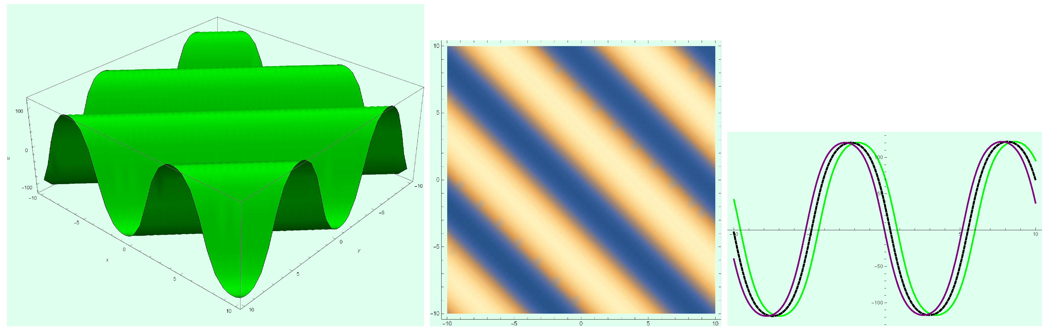
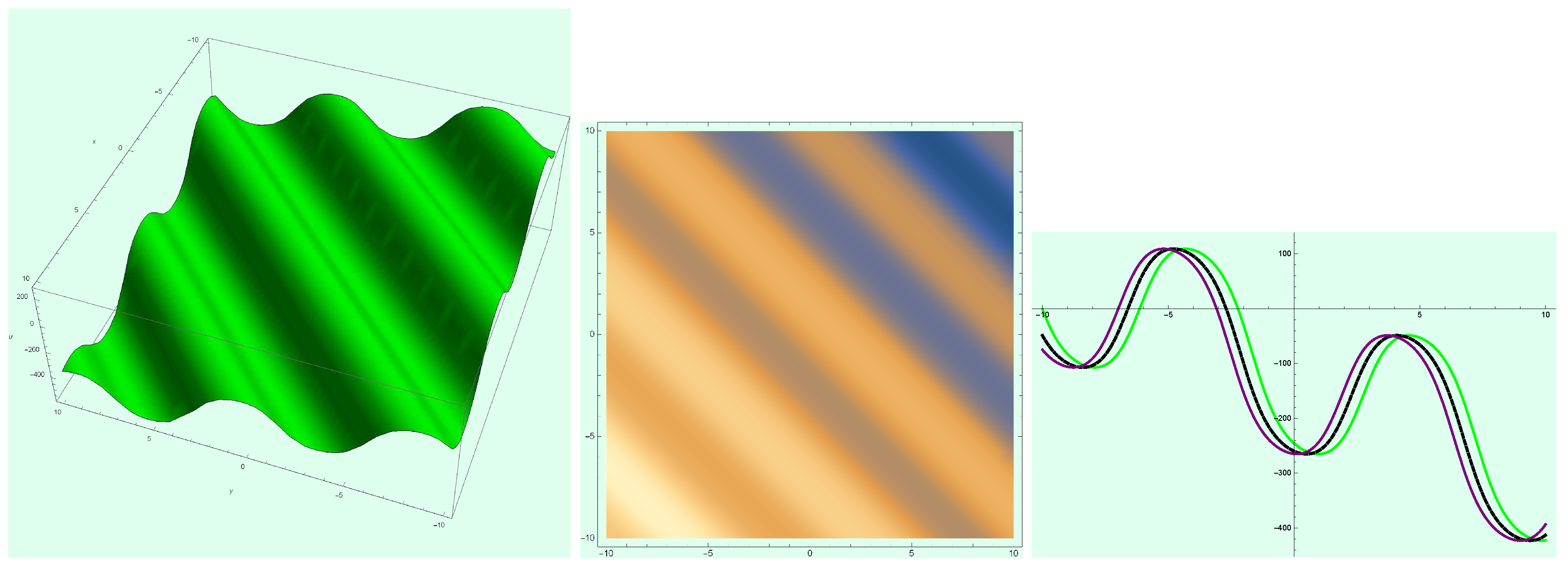
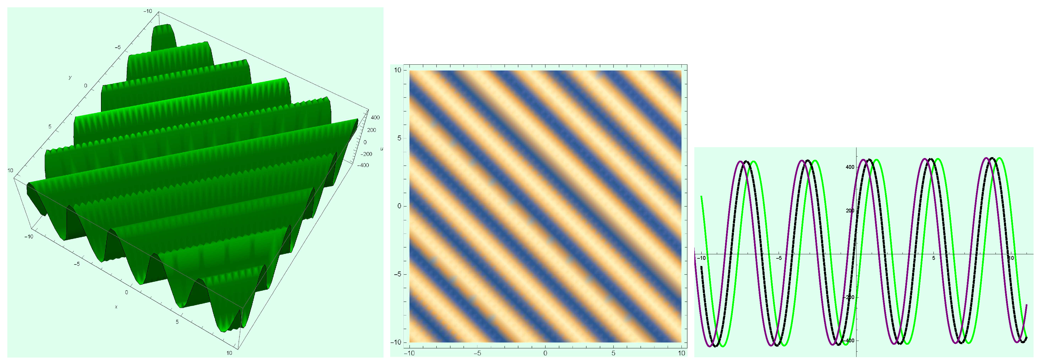
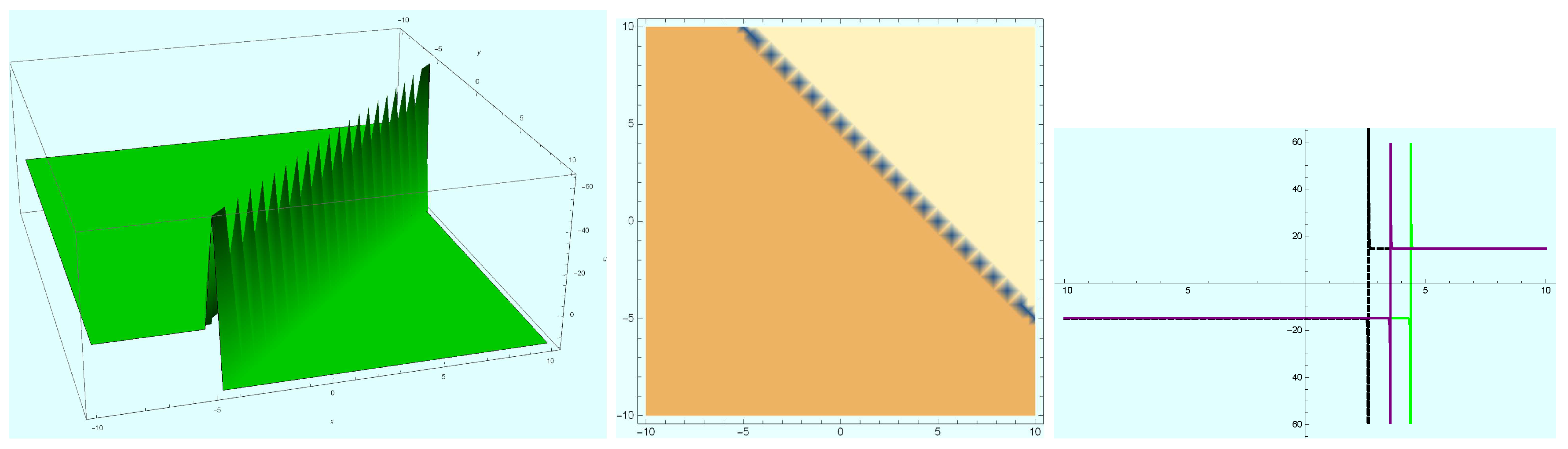
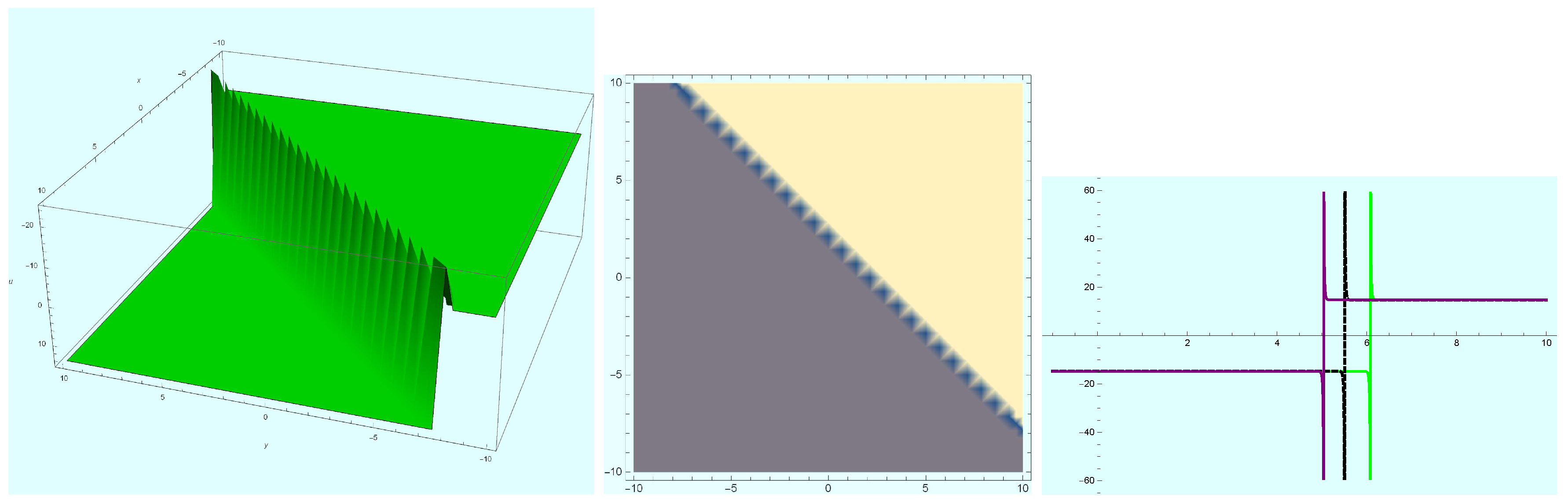
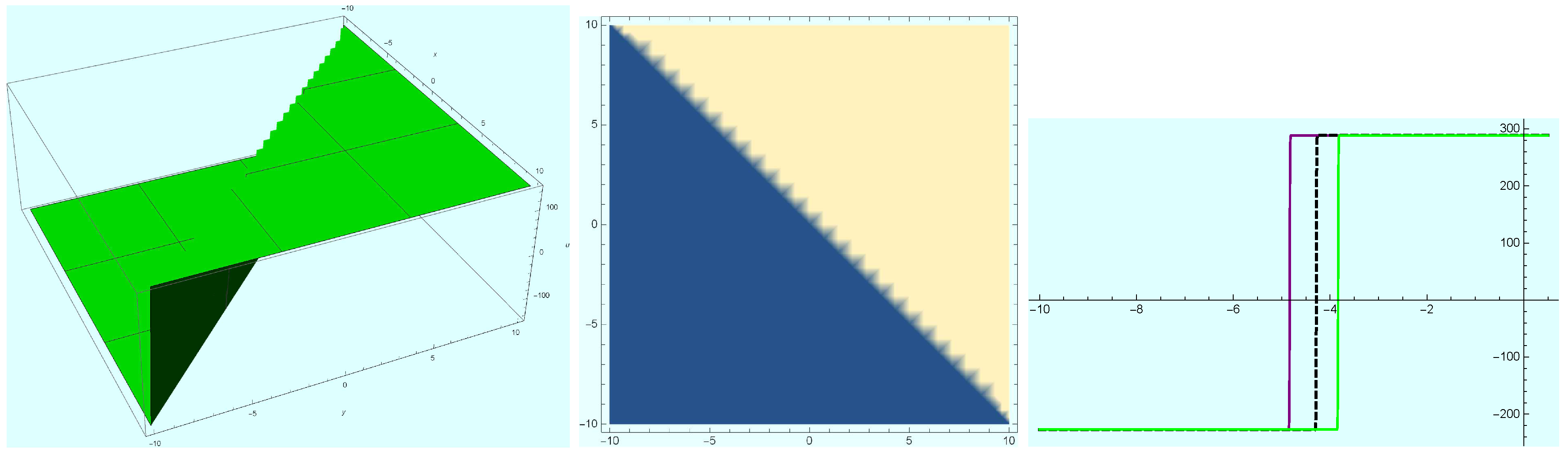
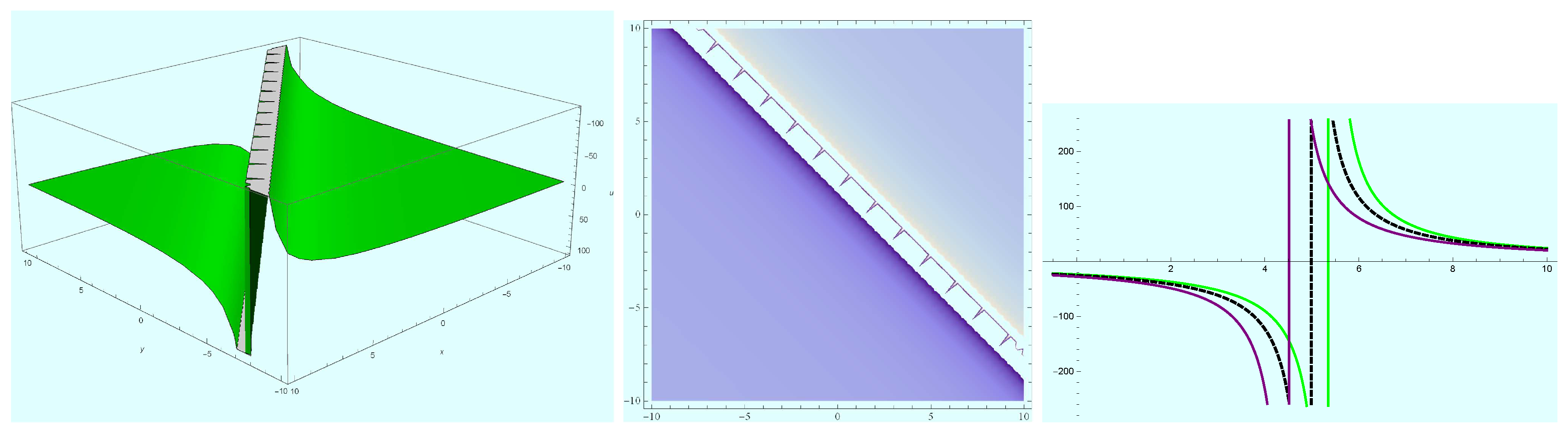
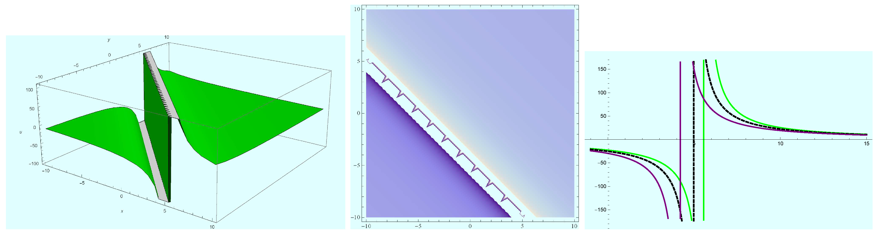
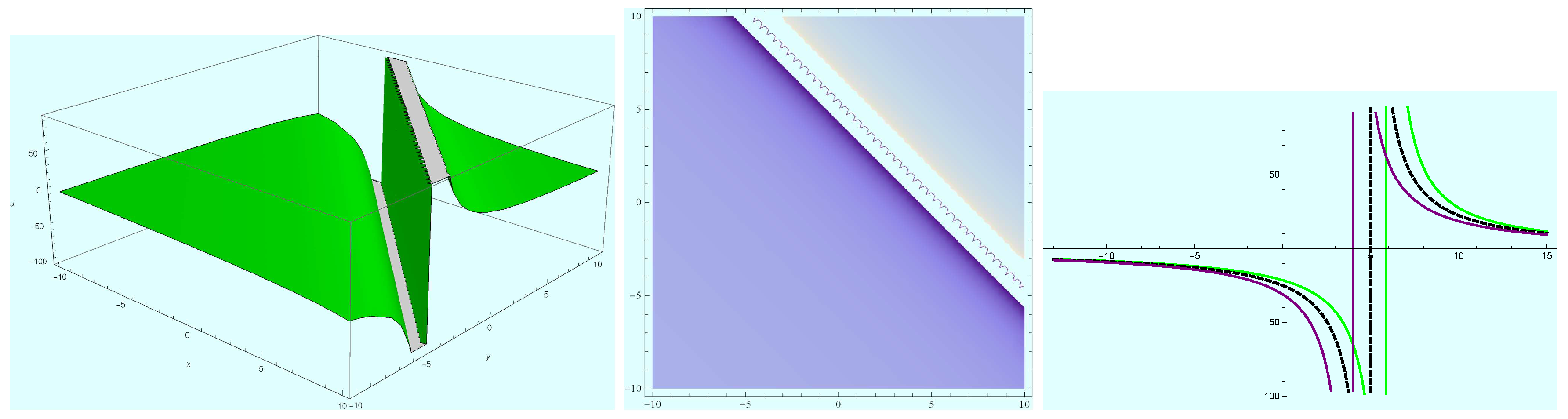
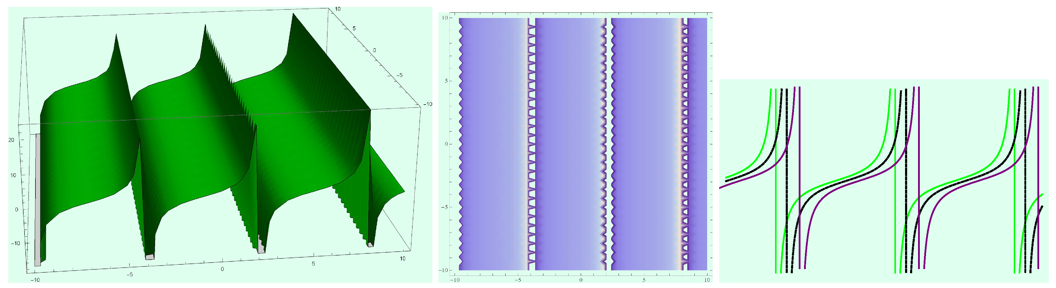
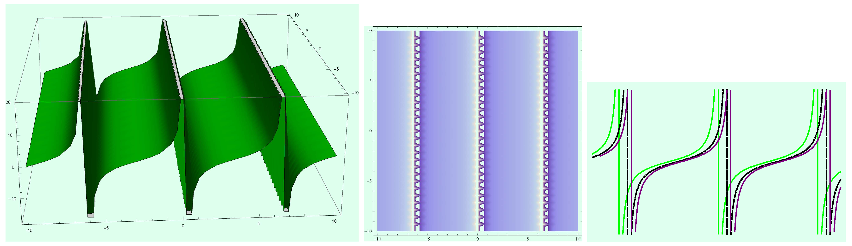
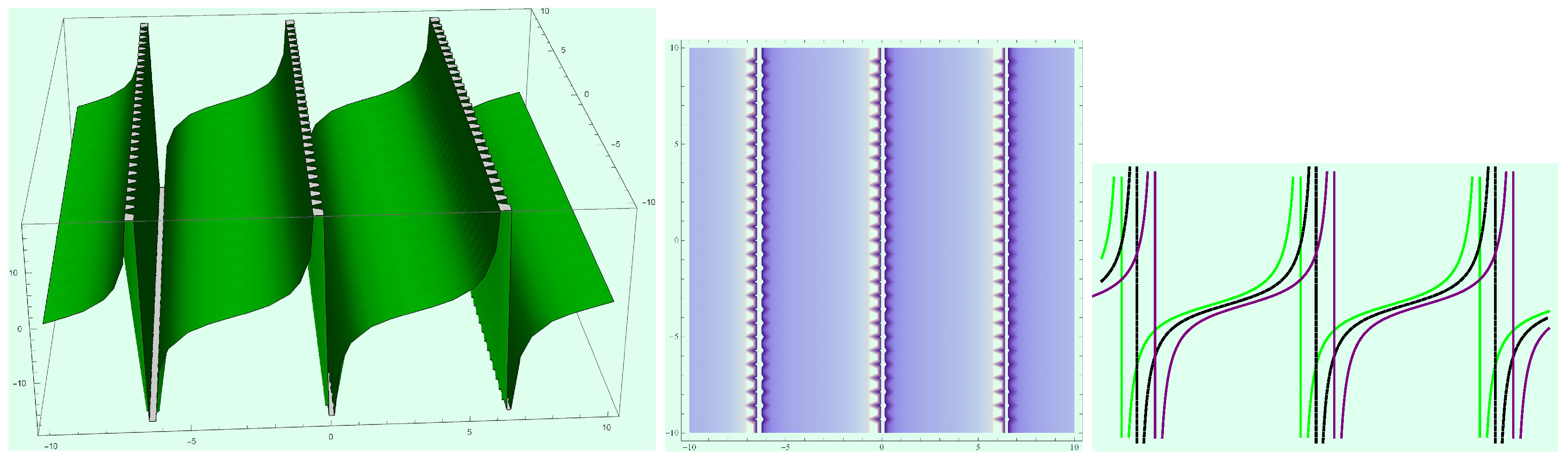
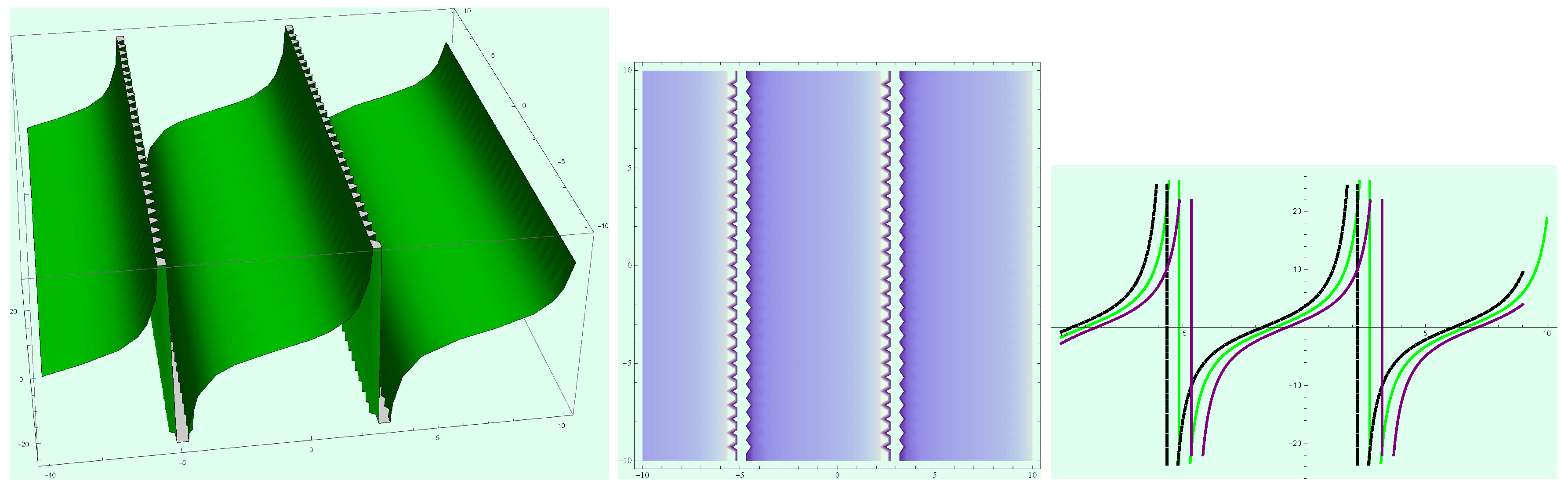
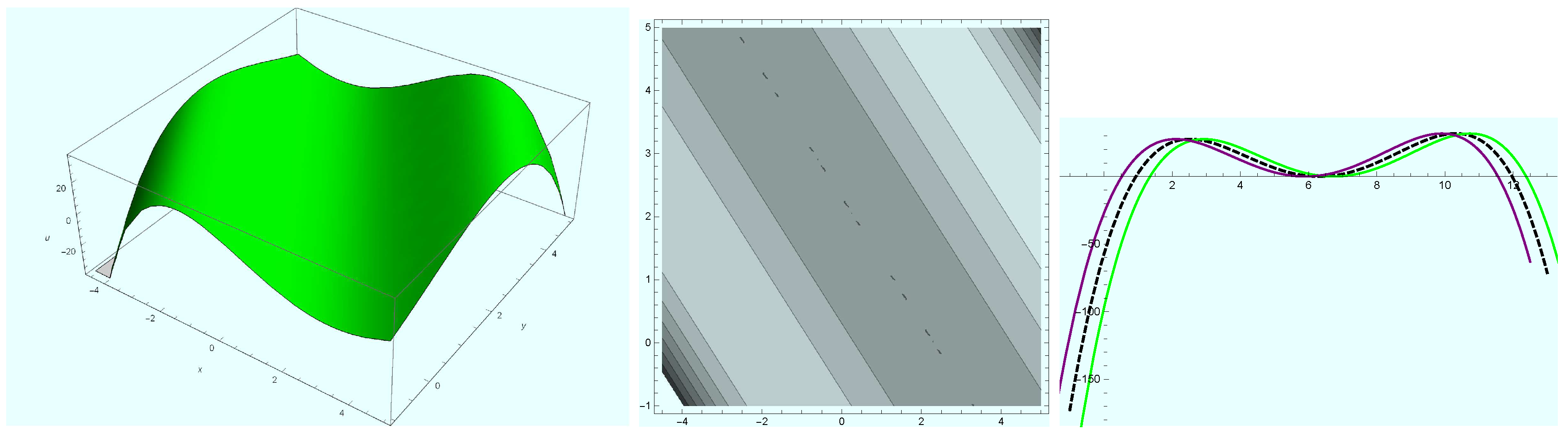
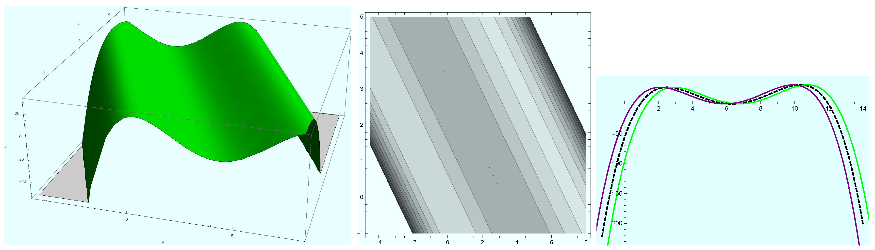
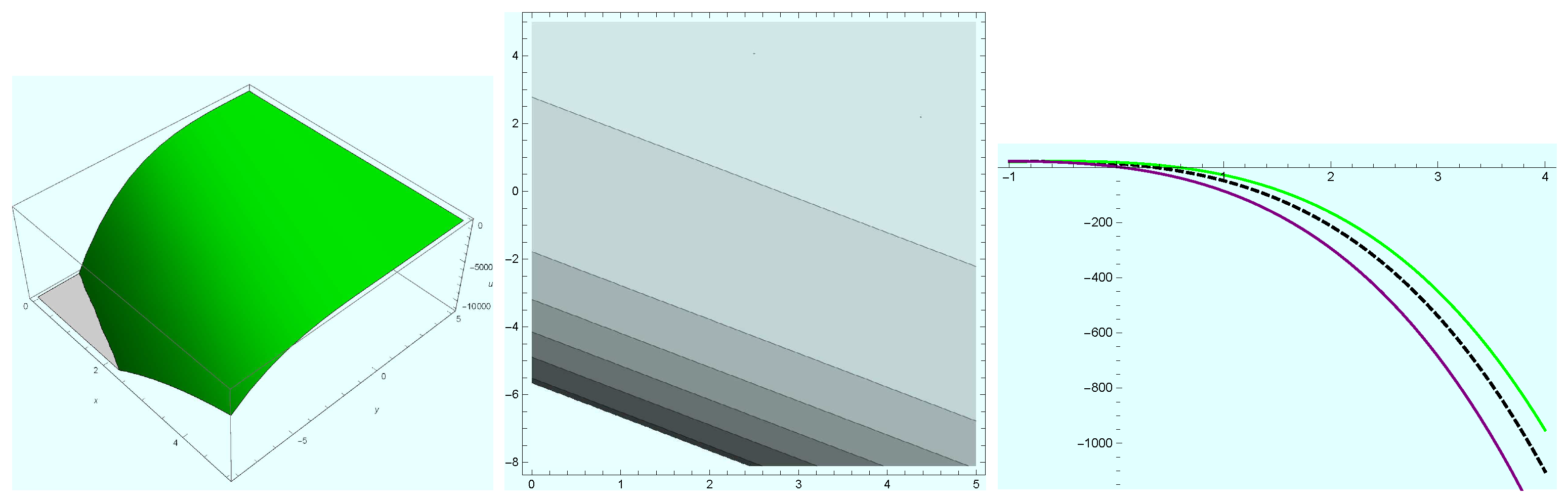
4. Discussion of the Graphical Representations of Solutions Obtained for 3D-gBSe (2)

The dynamics of solutions in the model of the generalized (3+1)-dimensional breaking soliton equation are described graphically. In a bid to gain better knowledge regarding the physical properties of the secured results, the derived solutions were depicted by choosing different values of parameters. For instance, the 3D-plot, density plot and 2D-plot of the periodic soliton solution (20) are represented with different values of parameters in Figure 1, where we assign values to the constants; in Figure 1, we let $\omega =0.2$, $\nu =0.6$, $r_1=100$, $r_2=50.05$, $r_3=20.05$, $Q=10$, $R=70$ and $C_3=1$; in Figure 1 we made $\omega =0.2$, $\nu =0.6$, $r_1=90$, $r_2=40.05$, $r_3=0.05$, $Q=10$, $R=70$ and $C_3=1$; and in Figure 3 we assumed $\omega =0.2$, $\nu =0.6$, $r_1=100$, $r_2=50.05$, $r_3=-80$, $Q=10$, $R=70$ and $C_3=1$,. In addition, we varied the values of t and z such that they were allocated values $t=-10$, $z=-1$, $t=-11$, and $z=0$; and $t=-25$ and $z=-9$ for the Figures respectively. It is observable that the wave deflection changes as time t reduces from $-10$ to $-25$.

Furthermore, the singular soliton solutions (24) obtained in the form of hyperbolic and trigonometric functions were plotted. 3D, density and 2D plots of (24) were done by setting positive values to the constants; in Figure 4 we supposed $\lambda =-0.08$, $\omega =2.02$, $\nu =2.02$, $\alpha =30$, $\mu =10.125$, $\beta =20.2$, $C_1=0.5$ and $C_2=2.3$; in Figure 5 we let $\lambda =-0.08$, $\omega =2.02$, $\nu =0.02$, $\alpha =30$, $\mu =10.125$, $\beta =20.2$, $C_1=1$ and $C_2=2$; and in Figure 6 we assumed $\lambda =0.0008$, $\omega =-0.02$, $\nu =0.02$, $\alpha =300$, $\mu =0.125$, $\beta =200.2$, $C_1=1$ and $C_2=0.8$. More so, we randomized t and z in which the figures respectively have $t=1$, $z=0$, $t=2$ and $z=-3.5$; and $t=-0.2$ and $z=20$. Figure 7 shows the 3D, density and 2D-plots of solution (25) with a singularity when $t=2.1$ and $z=-3$; Figure 8 reflects the same with a singularity when $t=-6$ and $z=25$; and Figure 9 exhibits (25) with a singularity at $t=4$, $z=30$. Other parameters involved were allotted values: $\lambda =-0.02$, $\omega =2.02$, $\nu =0.02$, $\mu =-0.005$, $\alpha =0.025$, $\beta =1$, $C_1=0$ and $C_2=2$; in Figure 7, $\lambda =-0.02$, $\omega =2.02$, $\nu =0.02$ and $\mu =-0.005$; in Figure 8, $\alpha =0.025$, $\beta =1$, $C_1=0.1$ and $C_2=2$; and in Figure 9, $\lambda =-0.02$, $\omega =2.02$, $\nu =0.02$, $\mu =-0.005$, $\alpha =0.025$, $\beta =1$, $C_1=0.1$ and $C_2=2$.

In addition, we made graphical demonstrations of the soliton solution (27) with singularities, by using 3D-plots, density plots and 2D-plots. In this case, we allocated values to the constants; for instance, in Figure 10 we let $\omega =0.48$, $\nu =0$, $\alpha =0.2$, $\beta =4$, $B_0=0$, $t=1$ and $x=2$; in Figure 11 we put $\omega =0.51$, $\nu =0$, $\alpha =0.5$, $\beta =4$, $B_0=0$, $t=0$ and $x=3$. In Figure 12 we assumed $\omega =0.51$, $\nu =0$, $\alpha =0.5$, $\beta =4$, $B_0=0$, $t=-1$ and $x=-4$.

Moreover, Figure 13 displays 3D, density and 2D-plots pictorial representation of soliton solution (28) with singularities when $\omega =0.48$, $\nu =0$, $\alpha =0.2$, $\beta =4$, $B_0=0$, $t=1$ and $x=4$. Figure 14 also reveals the 3D-plot, density and 2D-plots graphic display of (28) with singularities when $\omega =0.48$, $\nu =0$, $\alpha =0.2$, $\beta =4$, $B_0=0$, $t=0$ and $x=-4$. Besides, with $\omega =0.6$, $\nu =0$, $\alpha =0.2$, $\beta =4$, $B_0=0$, $t=-6$ and $x=7$, we show 3D, density and 2D-plots of Figure 15.

Finally, we show the solitary wave profile of series solution (34) with 3D-plot, density plot and 2D-plot in Figure 16 when $\omega =1.6$, $\nu =0.3$, $c_0=0$, $c_1=-0.2$, $c_2=7.825$, $c_3=-0.125$, $P=1.8$, $Q=83$, $R=25$, $t=1.6$ and $z=1.1$. Figure 17 exhibits the 3D, density and 2D plots of solution (34) when $\omega =1.6$, $\nu =0.4$, $c_0=0$, $c_1=-0.2$, $c_2=10.825$, $c_3=-0.125$, $P=10.8$, $Q=83$, $R=25$, $t=-1$ and $z=-8$. When $\omega =0.1$, $\nu =0.4$, $c_0=0$, $c_1=-0.2$, $c_2=8.825$, $c_3=-0.125$, $P=10.8$, $Q=83$, $R=25$, $t=5$ and $z=4$ Figure 18 shows 3D-plot, density and 2D-plots of series solution (34).

We can see that the changes in the parameters cause clear and obvious effects on the dynamics of the solitons and the series solutions. By making a comparison of the results secured in this work and those of the previous studies, it was revealed that the solutions gained here are completely different.

5. Conclusions

In this article, we investigated a (3+1)-dimensional generalized breaking soliton Equation (2). We constructed exact solutions for Equation (2) via the implementation of Lie symmetry reductions, direct integration, $(G^{\prime }/G)$-expansion and power series solution methods. Solutions obtained were in the form of trigonometric, hyperbolic functions and Jacobi elliptic functions. Moreover, the graphical representations of the solutions were shown with various values of the parameters and t, x and z to give a view of the wave dynamical appearances of the solutions. Lastly, we constructed the conserved vectors of Equation (2) through the engagement of the general multiplier method and Ibragimov’s theorem. The results of this paper could be of interest to scientists working in the fields of engineering and nonlinear sciences.

References

1. Wazwaz, A.M. Multiple optical kink solutions for new Painlevé integrable (3+1)-dimensional sine-Gordon equations with constant and time-dependent coefficients. Optik 2020, in press. [Google Scholar]
2. Wazwaz, A.M. Painlevé analysis for new (3+1)-dimensional Boiti-Leon-Manna-Pempinelli equations with constant and time-dependent equations. Int. Numer. Methods Heat Fluid Flow 2019, 30, 996–1008. [Google Scholar] [CrossRef]
3. Motsepa, T.; Khalique, C.M. Closed-form solutions and conserved vectors of the (3+1)-dimensional negative-order KdV equation. Adv. Math. Model. Appl. 2020, 5, 7–18. [Google Scholar]
4. Wazwaz, A.M.; Xu, G.Q. Integrability aspects and localized wave solutions for a new (4+1)-dimensional Boiti-Leon-Manna-Pempinelli equation. Nonlinear Dyn. 2019, 98, 1379–1390. [Google Scholar]
5. Gandarias, M.L.; Rosa, M.; Khalique, C.M. Conservation laws and travelling wave solutions for double dispersion equations in (1+1) and (2+1) dimensions. Symmetry 2020, 12, 950. [Google Scholar] [CrossRef]
6. Mhlanga, I.E.; Khalique, C.M. A study of a generalized Benney-Luke equation with time-dependent coefficients. Nonlinear Dyn. 2017, 90, 1535–1544. [Google Scholar] [CrossRef]
7. Motsepa, T.; Khalique, C.M.; Gandarias, M.L. Symmetry analysis and conservation laws of the Zoomeron equation. Symmetry 2017, 9, 27. [Google Scholar] [CrossRef] [Green Version]
8. Zabusky, N.J.; Kruskal, M.D. Interaction of solitons in a collisionless plasma and recurrence of initial states. Phys. Rev. Lett. 1965, 15, 240–243. [Google Scholar] [CrossRef] [Green Version]
9. Ablowitz, M.J.; Clarkson, P.A. Solitons, Nonlinear Evolution Equations and Inverse Scattering; Cambridge University Press: Cambridge, UK, 1991. [Google Scholar]
10. Weiss, J.; Tabor, M.; Carnevale, G. The Painleve property and a partial differential equations with an essential singularity. Phys. Lett. A 1985, 109, 205–208. [Google Scholar]
11. Zheng, C.L.; Fang, J.P. New exact solutions and fractional patterns of generalized Broer-Kaup system via a mapping approach. Chaos Soliton Fract. 2006, 27, 1321–1327. [Google Scholar] [CrossRef]
12. Wen, X.Y. Construction of new exact rational form non-travelling wave solutions to the (2+1)-dimensional generalized BroerKaup system. Appl. Math. Comput. 2010, 217, 1367–1375. [Google Scholar] [CrossRef]
13. Gu, C.H. Soliton Theory and Its Application; Zhejiang Science and Technology Press: Hangzhou, China, 1990. [Google Scholar]
14. Zeng, X.; Wang, D.S. A generalized extended rational expansion method and its application to (1+1)-dimensional dispersive long wave equation. Appl. Math. Comput. 2009, 212, 296–304. [Google Scholar] [CrossRef]
15. Zhou, Y.; Wang, M.; Wang, Y. Periodic wave solutions to a coupled KdV equations with variable coefficients. Phys. Lett. A 2003, 308, 31–36. [Google Scholar] [CrossRef]
16. Wazwaz, A.M. The tanh and sine-cosine method for compact and noncompact solutions of nonlinear Klein Gordon equation. Appl. Math. Comput. 2005, 167, 1179–1195. [Google Scholar] [CrossRef]
17. Kudryashov, N.A.; Loguinova, N.B. Extended simplest equation method for nonlinear differential equations. Appl. Math. Comput. 2008, 205, 396–402. [Google Scholar] [CrossRef]
18. Hirota, R. The Direct Method in Soliton Theory; Cambridge University Press: Cambridge, UK, 2004. [Google Scholar]
19. Olver, P.J. Applications of Lie Groups to Differential Equations, 2nd ed.; Springer: Berlin, Germany, 1993. [Google Scholar]
20. Ibragimov, N.H. Elementary Lie Group Analysis and Ordinary Differential Equations; John Wiley & Sons: Chichester, NY, USA, 1999. [Google Scholar]
21. Zhang, L.; Khalique, C.M. Classification and bifurcation of a class of second-order ODEs and its application to nonlinear PDEs. Discret. Contin. Dyn. Syst. Ser. S 2018, 11, 777–790. [Google Scholar] [CrossRef]
22. Wang, M.; Li, X.; Zhang, J. The (G/G)—expansion method and travelling wave solutions for linear evolution equations in mathematical physics. Phys. Lett. A 2005, 24, 1257–1268. [Google Scholar]
23. Matveev, V.B.; Salle, M.A. Darboux Transformations and Solitons; Springer: New York, NY, USA, 1991. [Google Scholar]
24. Chen, Y.; Yan, Z. New exact solutions of (2+1)-dimensional Gardner equation via the new sine-Gordon equation expansion method. Chaos Solitons Fractals 2005, 26, 399–406. [Google Scholar] [CrossRef]
25. Kudryashov, N.A. Simplest equation method to look for exact solutions of nonlinear differential equations. Chaos Solitons Fractals 2005, 24, 1217–1231. [Google Scholar] [CrossRef] [Green Version]
26. Chargui, Y.; Trabelsi, A.; Chetouani, L. Exact solution of the (1+1)-dimensional Dirac equation with vector and scalar linear potentials in the presence of a minimal length. Phys. Lett. A 2010, 374, 531–534. [Google Scholar]
27. Khalique, C.M.; Adem, K.R. Exact solutions of the (2+1)-dimensional Zakharov-Kuznetsov modified equal width equation using Lie group analysis. Math. Comput. Model. 2011, 54, 184–189. [Google Scholar] [CrossRef]
28. Wazwaz, A.M. Multiple-soliton solutions for extended (3+1)-dimensional Jimbo-Miwa equations. Appl. Math. Lett. 2017, 64, 21–26. [Google Scholar] [CrossRef]
29. Kaur, L.; Wazwaz, A.M. Dynamical analysis of lump solutions for (3+1)-dimensional generalized KP-Boussinesq equation and its dimensionally reduced equations. Phys. Scr. 2018, 93, 075203. [Google Scholar] [CrossRef]
30. Ali, M.R.; Ma, W.X. New exact solutions of nonlinear (3+1)-dimensional Boiti-Leon-Manna-Pempinelli equation. Adv. Math. Phys. 2019, 2019, 7. [Google Scholar] [CrossRef] [Green Version]
31. Verma, P.; Kaur, L. Extended exp ( ϕ ( ξ ) ) -expansion method for generalized breaking soliton equation. In AIP Conference Proceedings; AIP Publishing LLC: Melville, NY, USA, 2020; Volume 2214. [Google Scholar]
32. Yildirim, Y.; Yasar, E. A (2+1)-dimensional breaking soliton equation: Solutions and conservation laws. Chaos Solitons Fract. 2018, 107, 146–155. [Google Scholar] [CrossRef]
33. Mei, J.; Zhang, H. New types of exact solutions for a breaking soliton equation. Chaos Solitons Fract. 2004, 20, 771–777. [Google Scholar] [CrossRef]
34. Yan-Ze, P.; Krishnan, E.V. Two classes of new exact solutions to (2+1)-dimensional breaking soliton equation. Commun. Theor. Phys. 2005, 44, 807. [Google Scholar]
35. Wazwaz, A.M. Breaking soliton equations and negative-order breaking soliton equations of typical and higher orders. Pramana 2016, 87, 68. [Google Scholar] [CrossRef]
36. Wazwaz, A.M. The (2+1) and (3+1)-dimensional CBS equations: Multiple soliton solutions and multiple singular soliton solutions. Z. Naturforsch A 2010, 65, 173–181. [Google Scholar] [CrossRef]
37. Darvishi, M.T.; Najafi, M.; Najafi, M. New exact solutions for the (3+1)-dimensional breaking soliton equation. Int. J. Math. 2010, 6, 134–137. [Google Scholar]
38. Al-Amr, M.O. Exact solutions of the generalized (2+1)-dimensional nonlinear evolution equations via the modified simple equation method. Comput. Math. Appl. 2015, 69, 390–397. [Google Scholar] [CrossRef]
39. Liu, X.Z.; Yu, J.; Lou, Z.M. Residual symmetry, CRE integrability and interaction solutions of the (3+1)-dimensional breaking soliton equation. Phys. Scr. 2018, 93, 085201. [Google Scholar] [CrossRef]
40. Bluman, G.W.; Cheviakov, A.F.; Anco, S.C. Applications of Symmetry Methods to Partial Differential Equations; Springer: New York, NY, USA, 2010. [Google Scholar]
41. Leveque, R.J. Numerical Methods for Conservation Laws, 2nd ed.; Birkhäuser-Verlag: Basel, Switzerland, 1992. [Google Scholar]
42. Sarlet, W. Comment on conservation laws of higher order nonlinear PDEs and the variational conservation laws in the class with mixed derivatives. J. Phys. A Math. Theor. 2010, 43, 458001. [Google Scholar] [CrossRef]
43. Ibragimov, N.H. Integrating factors, adjoint equations and Lagrangians. J. Math. Anal. Appl. 2006, 318, 742–757. [Google Scholar] [CrossRef] [Green Version]
44. Ibragimov, N.H. A new conservation theorem. J. Math. Anal. Appl. 2007, 333, 311–328. [Google Scholar] [CrossRef] [Green Version]
45. Motsepa, T.; Abudiab, M.; Khalique, C.M. A study of an extended generalized (2+1)-dimensional Jaulent-Miodek equation. Int. J. Nonlin. Sci. Num. 2018, 19, 391–395. [Google Scholar] [CrossRef]
46. Abramowitz, M.; Stegun, I. Handbook of Mathematical Functions; Dover: New York, NY, USA, 1972. [Google Scholar]
47. Kudryashov, N.A. Analytical Theory of Nonlinear Differential Equations; Institute of Computer Investigations: Moskow-Igevsk, Russia, 2004. [Google Scholar]
48. Gradshteyn, I.S.; Ryzhik, I.M. Table of Integrals, Series and Products, 7th ed.; Academic Press: New York, NY, USA, 2007. [Google Scholar]
49. Wang, G.; Liu, X.; Zhang, Y. Symmetry reduction, exact solutions and conservation laws of a new fifth-order nonlinear integrable equation. Commun. Nonlinear Sci. Numer. Simul. 2013, 18, 2313–2320. [Google Scholar] [CrossRef]
50. Liu, H.; Li, J. Lie symmetry analysis and exact solutions for the short pulse equation. Nonlinear Anal. 2009, 21, 26–33. [Google Scholar] [CrossRef]
51. Liu, H.; Li, J.; Zhang, Q.X. Lie symmetry analysis and exact solutions for general Burger’s equation. J. Comput. Appl. Math. 2009, 228, 1–9. [Google Scholar] [CrossRef] [Green Version]
52. Bruzón, M.S.; Gandarias, M.L. Travelling wave solutions of the K(m, n) equation with generalized evolution. Math. Meth. Appl. Sci. 2018, 41, 5851–5857. [Google Scholar] [CrossRef]
53. Cheviakov, A.F. Computation of fluxes of conservation laws. J. Eng. Math. 2010, 66, 153–173. [Google Scholar] [CrossRef] [Green Version]
54. Motsepa, T.; Khalique, C.M. Cnoidal and snoidal waves solutions and conservation laws of a generalized (2+1)-dimensional KdV equation. In Proceedings of the 14th Regional Conference on Mathematical Physics; World Scientific Publishing Co Pte Ltd.: Singapore, 2018; pp. 253–263. [Google Scholar]
55. Khalique, C.M.; Moleleki, L.D. A (3+1)-dimensional generalized BKP-Boussinesq equation: Lie group approach. Results Phys. 2019, 13, 2211–3797. [Google Scholar] [CrossRef]
56. Khalique, C.M.; Adeyemo, O.D. A study of (3+1)-dimensional generalized Korteweg-de Vries-Zakharov-Kuznetsov equation via Lie symmetry approach. Results Phys. 2020, 18, 103197. [Google Scholar] [CrossRef]
Figure 1. Evolution of periodic solution (20) at t = 10 and z = 1 .
Mathematics 08 01692 g001
Figure 2. Evolution of periodic solution (20) at t = 11 and z = 0 .
Mathematics 08 01692 g002
Figure 3. Evolution of periodic solution (20) at t = 25 and z = 9 .
Mathematics 08 01692 g003
Figure 4. Evolution of traveling wave of singular soliton solution (24) at t = 1 and z = 0 .
Mathematics 08 01692 g004
Figure 5. Evolution of traveling wave of singular soliton solution (24) at t = 2 and z = 3.5 .
Mathematics 08 01692 g005
Figure 6. Evolution of traveling wave of singular soliton solution (24) at t = 0.2 and z = 20 .
Mathematics 08 01692 g006
Figure 7. Evolution of traveling wave of singular soliton solution (25) at t = 2.1 and z = 3 .
Mathematics 08 01692 g007
Figure 8. Evolution of traveling wave of singular soliton solution (25) at t = 6 and z = 25 .
Mathematics 08 01692 g008
Figure 9. Evolution of traveling wave of singular soliton solution (25) at t = 4 and z = 30 .
Mathematics 08 01692 g009
Figure 10. Profile of traveling wave solution (27) with parameters t = 1 and x = 2 .
Mathematics 08 01692 g010
Figure 11. Profile of traveling wave solution (27) with parameters t = 0 and x = 3 .
Mathematics 08 01692 g011
Figure 12. Profile of traveling wave solution (27) with parameters t = 1 and x = 4 .
Mathematics 08 01692 g012
Figure 13. Profile of traveling wave solution (28) when t = 1 and x = 4 .
Mathematics 08 01692 g013
Figure 14. Profile of traveling wave solution (28) when t = 0 and x = 4 .
Mathematics 08 01692 g014
Figure 15. Profile of traveling wave solution (28) when t = 6 and x = 7 .
Mathematics 08 01692 g015
Figure 16. Evolution of traveling wave of series solution (34) at t = 1.6 and z = 1.1 .
Mathematics 08 01692 g016
Figure 17. Evolution of traveling wave of series solution (34) at t = 1 and z = 8 .
Mathematics 08 01692 g017
Figure 18. Evolution of traveling wave of series solution (34) at t = 5 and z = 4 .
Mathematics 08 01692 g018