A New Geometric Metric in the Shape and Size Space of Curves in R n

Abstract

Shape analysis of curves in ${\mathbb{R}}^n$ is an active research topic in computer vision. While shape itself is important in many applications, there is also a need to study shape in conjunction with other features, such as scale and orientation. The combination of these features, shape, orientation and scale (size), gives different geometrical spaces. In this work, we define a new metric in the shape and size space, ${\mathcal{S}}_2$, which allows us to decompose ${\mathcal{S}}_2$ into a product space consisting of two components: ${\mathcal{S}}_4\times \mathbb{R}$, where ${\mathcal{S}}_4$ is the shape space. This new metric will be associated with a distance function, which will clearly distinguish the contribution that the difference in shape and the difference in size of the elements considered makes to the distance in ${\mathcal{S}}_2$, unlike the previous proposals. The performance of this metric is checked on a simulated data set, where our proposal performs better than other alternatives and shows its advantages, such as its invariance to changes of scale. Finally, we propose a procedure to detect outlier contours in ${\mathcal{S}}_2$ considering the square-root velocity function (SRVF) representation. For the first time, this problem has been addressed with nearest-neighbor techniques. Our proposal is applied to a novel data set of foot contours. Foot outliers can help shoe designers improve their designs.

1. Introduction

Shape analysis of curves in ${\mathbb{R}}^n$, where $n\ge 2$, is an important branch in many applications, including computer vision and medical imaging. Using the landmark representation of objects, Dryden et al. [1] studied the joint shape and size features of objects. However, an over-abundance of digital data, especially image data, is prompting the need for a different kind of shape analysis. In particular, the representation of shapes as elements of infinite-dimensional Riemannian manifolds with a given metric is of interest at this time and has important applications [2,3]. More recently, Srivastava et al. [4] presented a special representation of curves, called the square-root velocity function, or SRVF, under which a specific elastic metric becomes an $L^2$ metric and simplifies the shape analysis. This approach was analyzed by Kurtek et al. [5] on different scenarios, corresponding to different combinations of physical properties of the curves: shape, size, location and orientation. When the metric used in these infinite-dimensional spaces is invariant with respect to scaling, translation, rotation and reparameterization, the Riemannian manifold that represents the space of curves is known as the shape space, and following the notation of [5] will be denoted as ${\mathcal{S}}_4$. However, in many of the applications, other features such as orientation or size (scale) also play important roles and need to be incorporated into the underlying framework. A prime example is medical imaging, where the size of the anatomical structure of interest can provide important diagnostic information. In the case where the curve length (size) is considered, the feature space is called the shape and size (or shape and scale) space and will be denoted as ${\mathcal{S}}_2$ [5]. Other spaces denoted as ${\mathcal{S}}_1$ and ${\mathcal{S}}_3$ consider also changes in the orientations of the curves [5]. In this work, we will focus on the shape space ${\mathcal{S}}_4$ and the shape and size space ${\mathcal{S}}_2$, which are in general, completely different infinite-dimensional Riemannian manifolds. Curves in $S_2$ are different elements of the space if their shape or scale are different. Curves in $S_4$ are different elements of the space if their shape is different.

It seems natural, however, that the distance between two curves in space ${\mathcal{S}}_2$ should be related to the distance of these same curves in space ${\mathcal{S}}_4$. We can thereby discern whether the distance between the curves in space ${\mathcal{S}}_2$ is due, to a greater extent, to their difference in size or to their difference in shape.

In this sense, in [6], the Sobolev-type metric given in [3] for the shape space of planar closed curves is extended to the space of all planar closed curves where the metric considered exhibits a decomposition of the space of closed planar curves into a product space consisting of three components; that is, centroid translations, scale changes and curves in the shape space.

In this approach, we will consider representations of curves in ${\mathbb{R}}^n$ from square-root velocity functions (SRVF). Using these representations, we will consider two feature spaces studied in [5]: the shape space ${\mathcal{S}}_4$ and the shape and size space ${\mathcal{S}}_2$. The metric in ${\mathcal{S}}_4$ will be the same as in [5]; however, we propose a new metric in ${\mathcal{S}}_2$, which is completely different to the metric considered in [5]. This metric enjoys the property that ${\mathcal{S}}_2$ can be decomposed into a product space consisting of two components: ${\mathcal{S}}_4\times \mathbb{R}$, where the second space is related to the length (size) of the curve.

The outline of the paper is as follows: In Section 2, we review the SRVF representation of curves and the standard elastic metrics. In Section 3, we introduce the new metric in ${\mathcal{S}}_2$. The mean shape and geodesics with this new metric are introduced in Section 4 and Section 5, respectively. A comparison of the proposed metric and the standard elastic metric is carried out in Section 6 in a controlled setting with simulated curves, where we show the advantages of our proposal. We propose a procedure to detect outlier contours in ${\mathcal{S}}_2$ considering the SRVF representation. To the best of our knowledge, this is the first time this problem has been addressed with nearest-neighbor (NN) techniques. This is introduced in Section 7. Not only that, but so far outlier detection (in the multivariate context) in Anthropometry has only been used as a cleaning technique, for correcting or removing the outliers before analyzing data in the multivariate context [7,8]. However, outliers report very valuable information in the footwear design process: outliers can indicate which kinds of feet are more different from the rest and could therefore cause fitting problems in footwear if the design is not appropriate. In Section 8, our proposal is applied to a novel data set of foot contours. Finally, Section 9 contains the conclusions.

The code and data for reproducing the results are available at http://www3.uji.es/~epifanio/RESEARCH/metric.zip.

2. Classical Spaces of Curves in ${\mathbb{R}}^n$ for the SRVF Representation

In this section, we review some results from [9]. In particular, we consider the SRVF representation of curves in ${\mathbb{R}}^n$ and we summarize the main results for the shape space, ${\mathcal{S}}_4$, and for the shape and size space, ${\mathcal{S}}_2$, with the standard elastic metrics.

Let $\beta :[0,1]⟶{\mathbb{R}}^n$ be a parameterized curve that is absolutely continuous on $[0,1]$. The square-root velocity (SRVF) of $\beta$ is defined as the function $q:[0,1]⟶{\mathbb{R}}^n$ given by:

$$q\left(t\right)=\frac{{\beta }^{\prime }\left(t\right)}{\sqrt{|{\beta }^{\prime }\left(t\right)|}}.$$

(1)

As it can be seen in [9], this representation exists even where $|{\beta }^{\prime }\left(t\right)|=0$.

For every $q\in {\mathbb{L}}^2([0,1],{\mathbb{R}}^n)$, there is a curve $\beta$ (unique up to translation) such that the given q is the SRVF function of that $\beta$. In fact,

$$\beta \left(t\right)={\int }_0^{t}q\left(s\right)|q\left(s\right)|ds.$$

(2)

If a curve $\beta$ is of length one, then ${\int }_0^1{|q\left(t\right)|}^{2}dt=1$. Furthermore, the hypersphere

$${\mathcal{C}}^0=\left\{q:[0,1]⟶{\mathbb{R}}^n|{\int }_0^1{|q\left(t\right)|}^{2}dt=1\right\},$$

(3)

is a Hilbert manifold.

One way to study the shape and size (scale) space of open curves is to consider as a pre-shape space ${\mathbb{L}}^2={\mathbb{L}}^2([0,1],{\mathbb{R}}^n)$ with the usual inner product. To take care of the rotation and reparameterization of the curve $\beta$, we remember that a rotation is an element of $SO\left(n\right)$, the special orthogonal group of $n\times n$ matrices; and a reparameterization is an element of $\mathsf{\Gamma }=\{\gamma :[0,1]\to [0,1]|:\gamma \left(0\right)=0,\gamma \left(1\right)=1,\gamma$ is a diffeomorphism}.

The action of a reparameterization $\gamma \in \mathsf{\Gamma }$ transforms the curve $\beta :[0,1]\to {\mathbb{R}}^n$ to the curve $t\mapsto \beta \left(\gamma \right(t\left)\right)$. Hence, by the definition of the SRVF of a curve, we define the action of $\gamma \in \mathsf{\Gamma }$ in ${\mathcal{C}}_0$ by

$$\gamma \left(q\left(t\right)\right):=q\left(\gamma \left(t\right)\right)\sqrt{{\gamma }^{\prime }\left(t\right)}.$$

Likewise, the action of $O\in SO\left(n\right)$ on $q\in {\mathcal{C}}^0$ is just $O\left(q\right)\left(t\right)=O\left(q\right(t\left)\right).$ We shall denote the combined action

$$(O,\gamma )q\left(t\right):=O\left(q\left(\gamma \left(t\right)\right)\right)\sqrt{{\gamma }^{\prime }\left(t\right)},O\in SO\left(n\right),\gamma \in \mathsf{\Gamma }.$$

The orbit of a function $q\in {\mathbb{L}}^2$ is

$$\left[q\right]=\left\{(O,\gamma )\left(q\right)|(O,\gamma )\in SO(n)\times \mathsf{\Gamma }\right\}.$$

(4)

If we consider the metric in ${\mathbb{L}}^2$ given by the usual inner product

$${\langle v_1,v_2\rangle }_{L^2}={\int }_0^1\langle v_1\left(t\right),v_2\left(t\right)\rangle dt,$$

(5)

the feature space of interest is:

$${\mathcal{S}}_2=\left\{\left[q\right]/q\in {\mathbb{L}}^2\right\},$$

(6)

and the distance in ${\mathcal{S}}_2$ is:

$$d_2(\left[q_1\right],\left[q_2\right])=\underset{O\in SO\left(n\right),\gamma \in \mathsf{\Gamma }}{inf}{|q_1-(O,\gamma )\left(q_2\right)|}_{{\mathbb{L}}^2}.$$

(7)

Then, the geodesic between $q_1$ and the optimal reparameterization of $q_2$, which is denoted as $q_2^{*}=(O,{\gamma }^{*})\left(q_2\right),$ is

$${\mathsf{\Psi }}_{\tau }=(1-\tau )q_1+\tau q_2^{*},\tau \in \mathbb{R}.$$

(8)

On the other hand, the shape space (without considering the size (scale) of the curves) is

$${\mathcal{S}}_4=\{\left[q\right]|q\in {\mathcal{C}}^0\}.$$

(9)

The distance in ${\mathcal{S}}_4$ is given by

$$d_4(\left[q_1\right],\left[q_2\right])=\underset{O\in SO\left(n\right),\gamma \in \mathsf{\Gamma }}{inf}{cos}^{-1}\left({\langle q_1,(O,\gamma )\left(q_2\right)\rangle }_{{\mathbb{L}}^2}\right),$$

(10)

and the geodesic between $q_1$ and $q_2^{*}$ is

$$\alpha \left(\tau \right)=\frac{1}{sin\theta }\left(sin\left(\theta (1-\tau )\right)q_1+sin\left(\theta \tau \right)q_2^{*}\right),$$

(11)

where $\theta ={cos}^{-1}{\langle q_1,q_2^{*}\rangle }_{{\mathbb{L}}^2}$.

3. A New Metric in the Shape and Size Space of Curves in ${\mathbb{R}}^n$

When ${\mathcal{S}}_2$ is considered as shape and size space, it is difficult to distinguish whether the distance between two shapes $\left[q_1\right]$ and $\left[q_2\right]$ is due to the difference in shape or to the difference in size between the corresponding curves ${\beta }_1$ and ${\beta }_2$. We are therefore going to consider another shape-size space for curves that will be isometric to ${\mathcal{S}}_2$ with another appropriate product metric.

Instead of considering in ${\mathbb{L}}^2$ the usual ${\mathbb{L}}^2$-metric given in Equation (5), if $q\in {\mathbb{L}}^2([0,1],{\mathbb{R}}^n)$, for any two vectors $v_1,v_2$ in $T_q{\mathbb{L}}^2\left([0,1]\right)\equiv {\mathbb{L}}^2([0,1],{\mathbb{R}}^n)$, we will consider the following metric to endow ${\mathbb{L}}^2\left([0,1]\right)$ with a Riemannian structure,

$$\widehat{g}(v_1,v_2):=\frac{1}{R^2\left(q\right)}{\langle v_1,v_2\rangle }_{L^2}.$$

(12)

where

$$R\left(q\right):={\left({\int }_0^1{|q\left(t\right)|}^{2}dt\right)}^{\frac{1}{2}}.$$

The case $R\left(q\right)=0$ will be excluded, which will mean that curves of length 0 are not considered in our space.

From this metric, we will endow (Theorem 1) ${\mathcal{C}}^0\times \mathbb{R}$ with a Riemannian structure in such a way that ${\mathcal{C}}^0\times \mathbb{R}$ will be isometric to $\left({\mathbb{L}}^2\left([0,1]\right),\widehat{g}\right).$ This isometry will be exported (Theorem 2) to an isometry between ${\mathcal{S}}_2$ and ${\mathcal{S}}_4\times \mathbb{R}$.

Therefore, we obtain a new metric which enjoys the property that ${\mathcal{S}}_2$ can be decomposed into a product space consisting of two components: ${\mathcal{S}}_4\times \mathbb{R}$, where the second space is related with the length (size) of the curve. This new metric is associated with a distance function, see Corollary 3, given by

$${\mathrm{d}}_{\mathrm{new}}(\left[p\right],\left[q\right])=\sqrt{{\mathrm{d}}_4^2\left(\left[\frac{p}{R\left(p\right)}\right],\left[\frac{q}{R\left(q\right)}\right]\right)+{ln}^2\left(\frac{R\left(p\right)}{R\left(q\right)}\right)}.$$

(13)

This distance is invariant under rotations and under rescaling in the sense that ${\mathrm{d}}_{\mathrm{new}}(O\left(\left[p\right]\right),O\left(\left[q\right]\right))={\mathrm{d}}_{\mathrm{new}}(\left[p\right],\left[q\right])$ and ${\mathrm{d}}_{\mathrm{new}}(\lambda \left[p\right],\lambda \left[q\right])={\mathrm{d}}_{\mathrm{new}}(\left[p\right],\left[q\right])$ for any O in $SO\left(n\right)$ and any $\lambda >0$.

3.1. An Isometry between ${\mathbb{L}}^2([0,1],{\mathbb{R}}^n)\backslash \{\overrightarrow{0}\}$ and ${\mathcal{C}}^0\times \mathbb{R}$

We will begin this section defining a function F which will provide an isometry between ${\mathbb{L}}^2([0,1],{\mathbb{R}}^n)\backslash \{\overrightarrow{0}\}$ and ${\mathcal{C}}^0\times \mathbb{R}$. We consider the smooth map

$$\begin{array}{cc}\hfill F:{\mathbb{L}}^2([0,1],{\mathbb{R}}^n)& \backslash \{\overrightarrow{0}\}\to {\mathcal{C}}^0\times \mathbb{R},\hfill \\ \hfill q& \mapsto F\left(q\right):=\left(\frac{q}{R\left(q\right)},lnR\left(q\right)\right).\hfill \end{array}$$

Observe that F is well defined for any ${\mathbb{L}}^2([0,1],{\mathbb{R}}^n))\backslash \{\overrightarrow{0}\}$ where

$$\{\overrightarrow{0}\}:=\left\{q\in {\mathbb{L}}^2([0,1],{\mathbb{R}}^n)/{\int }_0^1{|q\left(t\right)|}^{2}dt=0\right\}=R^{-1}\left(0\right).$$

The function F has immediate smooth inverse given by

$$\begin{array}{cc}\hfill F^{-1}:{\mathcal{C}}^0& \times \mathbb{R}\to {\mathbb{L}}^2([0,1],{\mathbb{R}}^n)\backslash \{\overrightarrow{0}\},\hfill \\ & (q,t)\mapsto F^{-1}(q,t)=e^{t}q.\hfill \end{array}$$

The Functions R, $\pi$ and F and Their Properties

Now we state some properties of the function R, some properties of $\pi \left(q\right):=\frac{1}{R\left(q\right)}q$ from ${\mathbb{L}}^2$ to ${\mathcal{C}}^0$, that is the natural projection given by the normalization of an SRVF using its norm, and some properties of the function F:

Proposition 1.

Properties of the functions R, π and F:

1. 

Given a curve $\beta \left(t\right)$ and $q\left(t\right)=\frac{{\beta }^{\prime }\left(t\right)}{\sqrt{|{\beta }^{\prime }\left(t\right)|}}$. Then, $R\left(q\right)=\sqrt{L\left(\beta \right)}$ is the square root of the length of the curve β.

2. 

For any $\gamma \in \mathsf{\Gamma }$,

$$R\left(q\left(\gamma \left(t\right)\right)\sqrt{{\gamma }^{\prime }\left(t\right)})\right)=R\left(q\left(t\right)\right).$$

3. 

For any $O\in \mathrm{SO}\left(n\right),$

$$R\left(O\right(q\left(t\right))=R(q\left(t\right)).$$

4. 

For any $O\in \mathrm{SO}\left(n\right)$,

$$\pi \left(Oq\right)=O\pi \left(q\right).$$

Namely, the rotation group commutes with the projection π.

5. 

For any $\lambda >0$

$$\pi \left(\lambda q\right)=\pi \left(q\right)$$

6. 

Given $(O,\gamma )\in \mathrm{SO}\left(n\right)\times \mathsf{\Gamma }$, and $q\in {\mathbb{L}}^2([0,1],{\mathbb{R}}^n)\backslash \{\overrightarrow{0}\}$ then

$$F\left(O\left(q\left(\gamma \left(t\right)\right)\right)\sqrt{{\gamma }^{\prime }\left(t\right)}\right)=\left(O\left(\pi \right(q\left(\gamma \right(t\left)\right)),lnR(q)\right).$$

7. 

F is smooth and admits smooth inverse with never vanishing differential map.

From the properties of $\pi$, R and F, we can conclude the following diffeomorphisms.

Corollary 1.

From the function F we have that

1. 

${\mathbb{L}}^2([0,1],{\mathbb{R}}^n)\backslash \{\overrightarrow{0}\}\stackrel{\mathit{diff}}{\sim }{\mathcal{C}}^0\times \mathbb{R}.$

2. 

Since ${\mathcal{S}}_2={\mathbb{L}}^2/\mathsf{\Gamma }\times \mathrm{SO}\left(n\right)$, then

$${\mathcal{S}}_2\backslash \{\overrightarrow{0}\}\stackrel{\mathit{diff}}{\sim }\left({\mathcal{C}}^0/\mathsf{\Gamma }\times \mathrm{SO}\left(n\right)\right)\times \mathbb{R}\stackrel{\mathit{diff}}{\sim }{\mathcal{S}}_4\times \mathbb{R}.$$

As already mentioned at the beginning of the section, if $q\in {\mathbb{L}}^2([0,1],{\mathbb{R}}^n)\backslash \{0\}$, the tangent space at q can be identified with ${\mathbb{L}}^2([0,1],{\mathbb{R}}^n)$ itself,

$$T_q{\mathbb{L}}^2([0,1],{\mathbb{R}}^n)\backslash \{0\}\equiv {\mathbb{L}}^2([0,1],{\mathbb{R}}^n)$$

and for any two vectors $v_1,v_2$ in $T_q{\mathbb{L}}^2([0,1],{\mathbb{R}}^n)\backslash \{0\}$ we will use the following metric to endow ${\mathbb{L}}^2([0,1],{\mathbb{R}}^n)\backslash \{0\}$ with a Riemannian structure,

$$\widehat{g}(v_1,v_2):=\frac{1}{R^2\left(q\right)}{\langle v_1,v_2\rangle }_{L^2}.$$

(14)

Therefore, using $F^{-1}:{\mathcal{C}}^0\times \mathbb{R}\to {\mathbb{L}}^2([0,1],{\mathbb{R}}^n)\backslash \{\overrightarrow{0}\}$, we can pullback the metric $\widehat{g}$ to ${\widehat{g}}^{*}$ in ${\mathcal{C}}^0\times \mathbb{R}$ by the differential map $d{F}^{-1}:T_{(q,t)}{\mathcal{C}}^0\times \mathbb{R}\to T_{e^{t}p}{\mathbb{L}}^2([0,1],,{\mathbb{R}}^n)\backslash \{0\}$ in order to endow ${\mathcal{C}}^0\times \mathbb{R}$ with a Riemannian structure in such a way that $\left({\mathcal{C}}^0\times \mathbb{R},{\widehat{g}}^{*}\right)$ will be isometric to $\left({\mathbb{L}}^2([0,1],{\mathbb{R}}^n)\backslash \{0\},\widehat{g}\right)$.

Theorem 1.

There is an isometry $F:({\mathbb{L}}^2([0,1],{\mathbb{R}}^n)\backslash \{\overrightarrow{0}\},\widehat{g})⟶{\mathcal{C}}^0\times \mathbb{R}$ given by

$$F\left(p\right)=\left(\frac{p}{R\left(p\right)},lnR\left(p\right)\right),$$

(15)

where the usual product metric is considered in ${\mathcal{C}}^0\times \mathbb{R}$.

Proof. 

We have shown in Corollary 1 that F is a diffeomorphism; therefore, we only have to prove that the pullback ${\widehat{g}}^{*}$ of the metric $\widehat{g}$ is the usual product metric in ${\mathcal{C}}^0\times \mathbb{R}$.

$$T_{(q,t)}{\mathcal{C}}^0\times \mathbb{R}=T_q{\mathcal{C}}^0\oplus T_t\mathbb{R}$$

Given two vectors in $v_1,v_2\in T_{(q,t)}{\mathcal{C}}^0\times \mathbb{R}$ the pullback ${\widehat{g}}^{*}(v_1,v_2)$ is given by

$$\begin{array}{ccc}\hfill {\widehat{g}}^{*}(v_1,v_2)& & =\widehat{g}(d{F}^{-1}\left(v_1\right),d{F}^{-1}\left(v_2\right))=\hfill \\ & & =\frac{1}{R^2\left(e^{t}q\right)}{\langle d{F}^{-1}\left(v_1\right),d{F}^{-1}\left(v_2\right)\rangle }_{{\mathbb{L}}_2}.\hfill \end{array}$$

But

$$R^2\left(e^{t}q\right)={\int }_0^1|e^{t}q\left(s\right){|}^{2}ds=e^{2t}{\int }_0^1{|q|}^{2}ds=e^{2t},$$

because $q\in {\mathcal{C}}^0$. Therefore, for any two vectors $v_1,v_2\in T_{(q,t)}{\mathcal{C}}^0\times \mathbb{R}$

$${\widehat{g}}^{*}(v_1,v_2)=e^{-2t}{\langle d{F}^{-1}\left(v_1\right),d{F}^{-1}\left(v_2\right)\rangle }_{{\mathbb{L}}_2}.$$

Now, first of all, we need to prove that in the tangent space to ${\mathcal{C}}^0\times \mathbb{R}$ at $(q,t)$, $T_q{\mathcal{C}}^0$ is orthogonal to $T_t\mathbb{R}$. In order to do that, consider two vectors $v_1\in T_q{\mathcal{C}}^0$ and $v_2\in T_t\mathbb{R}$ and two curves ${\gamma }_1,{\gamma }_2:(-ϵ,ϵ)\to {\mathcal{C}}^0\times \mathbb{R}$, such that

$$\left\{\begin{array}{c}\hfill {\gamma }_1\left(s\right)=({\gamma }_1^1\left(s\right),t),{\gamma }_1\left(0\right)=(q,t),\frac{d}{ds}{\gamma }_1{\left(s\right)|}_{s=0}=v_1\\ \hfill {\gamma }_2\left(s\right)=(q,{\gamma }_2^2\left(s\right)),{\gamma }_1\left(0\right)=(q,t),\frac{d}{ds}{\gamma }_2{\left(s\right)|}_{s=0}=v_2\end{array}\right.$$

Then,

$$d{F}^{-1}\left(v_1\right)=\frac{d}{ds}{F}^{-1}\left({\gamma }_1\left(s\right)\right){{|}_{s=0}=\frac{d}{ds}\left(e^t{\gamma }_1^1\left(s\right)\right)|}_{s=0}=e^t{v}_1$$

with $v_1\in T_q{\mathcal{C}}^0$. Likewise,

$$\begin{array}{cc}\hfill d{F}^{-1}\left(v_2\right)=& \frac{d}{ds}{F}^{-1}\left({\gamma }_2\left(s\right)\right){{|}_{s=0}=\frac{d}{ds}\left(e^{{\gamma }_2^2\left(s\right)}q\right)|}_{s=0}\hfill \\ \hfill =& v_2{e}^{t}q\hfill \end{array}$$

where $v_2\in \mathbb{R},q\in {\mathcal{C}}^0$. Hence,

$$g^{*}(v_1,v_2)=e^{-2t}{\langle e^t{v}_1,v_2{e}^{t}q\rangle }_{{\mathbb{L}}_2}=v_2{\langle v_1,q\rangle }_{{\mathbb{L}}_2}=0$$

because ${\langle v_1,q\rangle }_{{\mathbb{L}}_2}=0$ for any $v_1\in T_q{\mathcal{C}}^0$.

Similarly if $v_1,v_2\in T_q{\mathcal{C}}^0$,

$${\widehat{g}}^{*}(v_1,v_2)=e^{-2t}{\langle e^t{v}_1,e^t{v}_2\rangle }_{{\mathbb{L}}_2}={\langle v_1,v_2\rangle }_{{\mathbb{L}}_2}$$

and if $v_1,v_2\in T_t\mathbb{R}$

$${\widehat{g}}^{*}(v_1,v_2)=e^{-2t}{\langle v_1{e}^{t}q,v_2{e}^{t}q\rangle }_{{\mathbb{L}}_2}=v_1{v}_2{\langle q,q\rangle }_{{\mathbb{L}}_2}=v_1{v}_2.$$

□

Since we are using the usual product metric in ${\mathcal{C}}^0\times \mathbb{R}$, we conclude the following result:

Corollary 2.

Let ${\mathrm{d}}_{\widehat{g}}$ denote the distance function in $({\mathbb{L}}^2([0,1],{\mathbb{R}}^n)\backslash \{\overrightarrow{0}\},\widehat{g})$, then

$$\begin{array}{ccc}\hfill {\mathrm{d}}_{\widehat{g}}(p,q)=& & \sqrt{{\mathrm{d}}_{{\mathcal{C}}^0}^2(\pi \left(p\right),\pi \left(q\right))+{\mathrm{d}}_{\mathbb{R}}^2(lnR\left(p\right),lnR\left(q\right))}\hfill \\ \hfill =& & \sqrt{{\mathrm{d}}_{{\mathcal{C}}^0}^2\left(\frac{p}{R\left(p\right)},\frac{q}{R\left(q\right)}\right)+{ln}^2\left(\frac{R\left(p\right)}{R\left(q\right)}\right)}\hfill \end{array}$$

(16)

where ${\mathrm{d}}_{{\mathcal{C}}^0}$ is the usual distance in ${\mathcal{C}}^0$.

From this explicit expression of the distance, it is easy to see that the metric $\widehat{g}$ is invariant under the action of reparameterizations and rotations.

Proposition 2.

The group $SO\left(n\right)\times \mathsf{\Gamma }$ acts isometrically on $({\mathbb{L}}^2([0,1],{\mathbb{R}}^n)\backslash \{\overrightarrow{0}\},\widehat{g})$.

Proof. 

We need to prove that

$$\begin{array}{cc}\hfill d_{\widehat{g}}\left((O,\gamma )\left(p\right),(O,\gamma )\left(q\right)\right)=& \sqrt{{\mathrm{d}}_{{\mathcal{C}}^0}^2\left(\frac{(O,\gamma )\left(p\right)}{R\left(\right(O,\gamma \left)\right(p\left)\right)},\frac{(O,\gamma )\left(q\right)}{R\left(\right(O,\gamma \left)\right(q\left)\right)}\right)+{ln}^2\left(\frac{R\left(\right(O,\gamma \left)\right(p\left)\right)}{R\left(\right(O,\gamma \left)\right(q\left)\right)}\right)}\hfill \\ \hfill =& {\mathrm{d}}_{\widehat{g}}(p,q),\forall (O,\gamma )\in SO\left(n\right)\times \mathsf{\Gamma }.\hfill \end{array}$$

By Proposition 1 we know that $R\left(\right(O,\gamma \left)\right(p\left)\right)=R\left(p\right)$ (and $R\left(\right(O,\gamma \left)\right(q\left)\right)=R\left(q\right)$). Hence, the proposition follows because

$$\begin{array}{cc}\hfill {\mathrm{d}}_{{\mathcal{C}}^0}^2\left(\frac{(O,\gamma )\left(p\right)}{R\left(\right(O,\gamma \left)\right(p\left)\right)},\frac{(O,\gamma )\left(q\right)}{R\left(\right(O,\gamma \left)\right(q\left)\right)}\right)=& {\mathrm{d}}_{{\mathcal{C}}^0}^2\left(\frac{(O,\gamma )\left(p\right)}{R\left(p\right)},\frac{(O,\gamma )\left(q\right)}{R\left(q\right)}\right)\hfill \\ \hfill =& {\int }_0^1{∥\frac{(O,\gamma )\left(p\right)\left(t\right)}{R\left(p\right)}-\frac{(O,\gamma )\left(q\right)\left(t\right)}{R\left(q\right)}∥}^{2}dt\hfill \\ \hfill =& {\int }_0^1{∥O\left(\left(\frac{p\left(\gamma \right(t\left)\right)}{R\left(p\right)}-\frac{q\left(\gamma \right(t\left)\right)}{R\left(q\right)}\right)\sqrt{{\gamma }^{\prime }\left(t\right)}\right)∥}^{2}dt\hfill \\ \hfill =& {\int }_0^1{∥\frac{p\left(\gamma \right(t\left)\right)}{R\left(p\right)}-\frac{q\left(\gamma \right(t\left)\right)}{R\left(q\right)}∥}^2{\gamma }^{\prime }\left(t\right)dt={\int }_0^1{∥\frac{p\left(\tau \right)}{R\left(p\right)}-\frac{q\left(\tau \right)}{R\left(q\right)}∥}^{2}d\tau \hfill \\ \hfill =& {\mathrm{d}}_{{\mathcal{C}}^0}^2\left(\frac{p}{R\left(p\right)},\frac{q}{R\left(q\right)}\right)\hfill \end{array}$$

□

3.2. The Isometry between ${\mathcal{S}}_2$ and ${\mathcal{S}}_4\times \mathbb{R}$

Using the isometry given by Theorem 1, an isometry between ${\mathcal{S}}_2$ and ${\mathcal{S}}_4\times \mathbb{R}$ can be constructed as stated in the following theorem:

Theorem 2.

The isometry F can be exported to an isometry $\left[F\right]$ by using the following commutative diagram

$$\begin{array}{ccc}{\mathbb{L}}^2([0,1],{\mathbb{R}}^n)\backslash \{\overrightarrow{0}\}& \stackrel{F}{\to }& {\mathcal{C}}^0\times \mathbb{R}\\ \phantom{{\mathsf{\Pi }}_1}\downarrow {\mathsf{\Pi }}_1& & \phantom{{\mathsf{\Pi }}_2}\downarrow {\mathsf{\Pi }}_2& & \\ {\mathcal{S}}_2\backslash \{0\}& \stackrel{\left[F\right]}{\to }& {\mathcal{S}}_4\times \mathbb{R}\end{array}$$

where ${\mathsf{\Pi }}_1\left(q\right)=\left[q\right]$ and ${\mathsf{\Pi }}_2(q,t)=(\left[q\right],t)$. Namely,

$$\left[F\right]\left[q\right]={\mathsf{\Pi }}_2\left(F\left(q\right)\right)$$

for any $q\in {\mathsf{\Pi }}_1^{-1}\left(\left[q\right]\right)$.

Proof. 

From Proposition 2 we know that $\mathrm{SO}\left(n\right)\times \mathsf{\Gamma }$ acts by isometries on $({\mathbb{L}}^2\backslash \{\overrightarrow{0}\},\widehat{g})$. Therefore, since the action of the group $\mathsf{\Gamma }\times SO\left(n\right)$ on $({\mathbb{L}}^2\backslash \{\overrightarrow{0}\},\widehat{g})$ and on ${\mathcal{C}}^0$ is by isometries, and bearing in mind the diffeomorphisms in Corollary 1, we obtain the result. □

The isometry $\left[F\right]$ of the above theorem can be used to obtain the expression of the new distance function.

Corollary 3.

Let ${\mathrm{d}}_{\mathrm{new}}$ denote the distance function in ${\mathcal{S}}_2\backslash \{\overrightarrow{0}\}$ when the isometry $\left[F\right]$ of Theorem 2 is considered, then

$$\begin{array}{ccc}\hfill {\mathrm{d}}_{\mathrm{new}}(\left[p\right],\left[q\right])=& & \sqrt{{\mathrm{d}}_4^2(\left[\pi \left(p\right)\right],\left[\pi \left(q\right)\right])+{\mathrm{d}}_{\mathbb{R}}^2(lnR\left(p\right),lnR\left(q\right))}\hfill \\ \hfill =& & \sqrt{{\mathrm{d}}_4^2\left(\left[\frac{p}{R\left(p\right)}\right],\left[\frac{q}{R\left(q\right)}\right]\right)+{ln}^2\left(\frac{R\left(p\right)}{R\left(q\right)}\right)}.\hfill \end{array}$$

(17)

In the following proposition we are proving that ${\mathrm{d}}_{\mathrm{new}}$ is a well defined distance function.

Proposition 3.

Let ${\mathrm{d}}_{\mathrm{new}}$ denote the distance function in ${\mathcal{S}}_2\backslash \{\overrightarrow{0}\}$ when the isometry $\left[F\right]$ of Theorem 2 is considered, then

1. 

${\mathrm{d}}_{\mathrm{new}}(\left[p\right],\left[q\right])={\mathrm{d}}_{\mathrm{new}}(\left[q\right],\left[p\right])$ for all $\left[p\right],\left[q\right]\in {\mathcal{S}}_2\backslash \overrightarrow{0}$.

2. 

${\mathrm{d}}_{\mathrm{new}}(\left[p\right],\left[q\right])=0$, if and only if, ${\mathrm{d}}_4\left(\left[\frac{p}{R\left(p\right)}\right],\left[\frac{q}{R\left(q\right)}\right]\right)=0$ and $R\left(p\right)=R\left(q\right)$.

3. 

For any $\left[p\right],\left[q\right],\left[r\right]\in {\mathcal{S}}_2\backslash \overrightarrow{0}$

$${\mathrm{d}}_{\mathrm{new}}(\left[p\right],\left[r\right])\le {\mathrm{d}}_{\mathrm{new}}(\left[p\right],\left[q\right])+{\mathrm{d}}_{\mathrm{new}}(\left[q\right],\left[r\right]).$$

4. 

${\mathrm{d}}_{\mathrm{new}}(\lambda \left[p\right],\lambda \left[q\right])={\mathrm{d}}_{\mathrm{new}}(\left[q\right],\left[p\right])$ for all $\left[p\right],\left[q\right]\in {\mathcal{S}}_2\backslash \overrightarrow{0}$, $\lambda \in \mathbb{R},\lambda \ne 0$.

Proof. 

Most of the statements of the proposition follows directly from the definition and the properties of ${\mathrm{d}}_4$ and R. We shall prove the triangle inequality for the sake of completeness. Let us denote by $\overrightarrow{v},\overrightarrow{w}\in {\mathbb{R}}^2$ the vectors given by

$$\overrightarrow{v}:=\left({\mathrm{d}}_4\left(\left[\frac{p}{R\left(p\right)}\right],\left[\frac{q}{R\left(q\right)}\right]\right),ln\left(\frac{R\left(p\right)}{R\left(q\right)}\right)\right),\overrightarrow{w}:=\left({\mathrm{d}}_4\left(\left[\frac{q}{R\left(q\right)}\right],\left[\frac{r}{R\left(r\right)}\right]\right),ln\left(\frac{R\left(q\right)}{R\left(r\right)}\right)\right)$$

Then, by applying the triangle inequality for ${\mathrm{d}}_4$,

$$\begin{array}{cc}\hfill {\left({\mathrm{d}}_{\mathrm{new}}(\left[p\right],\left[r\right])\right)}^2=& {\mathrm{d}}_4^2\left(\left[\frac{p}{R\left(p\right)}\right],\left[\frac{r}{R\left(r\right)}\right]\right)+{\left(ln\left(\frac{R\left(p\right)}{R\left(r\right)}\right)\right)}^2\hfill \\ \hfill \le & {\left({\mathrm{d}}_4\left(\left[\frac{p}{R\left(p\right)}\right],\left[\frac{q}{R\left(q\right)}\right]\right)+{\mathrm{d}}_4\left(\left[\frac{q}{R\left(q\right)}\right],\left[\frac{r}{R\left(r\right)}\right]\right)\right)}^2+{\left(ln\left(\frac{R\left(p\right)}{R\left(q\right)}\right)+ln\left(\frac{R\left(q\right)}{R\left(r\right)}\right)\right)}^2\hfill \\ \hfill =& \parallel \overrightarrow{v}+\overrightarrow{w}{\parallel }^2=\parallel \overrightarrow{v}{\parallel }^2+\parallel \overrightarrow{w}{\parallel }^2+2\parallel \overrightarrow{v}\parallel \parallel \overrightarrow{w}\parallel cos\left(\theta \right)\le \parallel \overrightarrow{v}{\parallel }^2+\parallel \overrightarrow{w}{\parallel }^2+2\parallel \overrightarrow{v}\parallel \parallel \overrightarrow{w}\parallel ={\left(\parallel \overrightarrow{v}\parallel +\parallel \overrightarrow{w}\parallel \right)}^2\hfill \\ \hfill =& {\left({\mathrm{d}}_{\mathrm{new}}(\left[p\right],\left[q\right])+{\mathrm{d}}_{\mathrm{new}}(\left[q\right],\left[r\right])\right)}^2.\hfill \end{array}$$

□

4. The Mean Shape

Given $\{{\beta }_1,\cdots ,{\beta }_n\}$, a sample of parameterized curves, and their corresponding SRVF, $\{q_1,\cdots ,q_n\}$, the Karcher mean shape regarding the new metric ${\mathrm{d}}_{\mathrm{new}}$ is defined as

$$\left[{\widehat{\mu }}_{new}\right]=argmi{n}_q\sum _{i=1}^n{\mathrm{d}}_{\mathrm{new}}{(\left[q\right],\left[q_i\right])}^2=argmi{n}_q\sum _{i=1}^n({\mathrm{d}}_4^2\left(\left[\frac{q}{R\left(q\right)}\right],\left[\frac{q_i}{R\left(q_i\right)}\right]\right)+{ln}^2\left(\frac{R\left(q\right)}{R\left(q_i\right)}\right)).$$

The value of $R\left(q\right)$ that minimizes ${\sum }_{i=1}^n{ln}^2\left(\frac{R\left(q\right)}{R\left(q_i\right)}\right)$ is the geometric mean of the $\{R\left(q_1\right),\cdots ,R\left(q_n\right)\}$, i.e., $\sqrt[n]{{\prod }_{i=1}^{n}R\left(q_i\right)},$ and a gradient-based approach for finding the value of $q/R\left(q\right)$ that minimizes

$$\sum _{i=1}^n{\mathrm{d}}_4^2\left(\left[\frac{q}{R\left(q\right)}\right],\left[\frac{q_i}{R\left(q_i\right)}\right]\right)$$

can be found in [10,11]. The detailed algorithm to find the Karcher mean in the shape space ${\mathcal{S}}_2$ can be found in [12].

Given ${\widehat{\mu }}_{C_0}$ the Karcher mean of ${\{q_i/R\left(q_i\right)\}}_{i=1,\cdots ,n}$ in the shape space, the Karcher mean in the shape and size space with the new metric is obtained as

$${\widehat{\mu }}_{new}={\widehat{\mu }}_{C_0}\sqrt[n]{\prod _{i=1}^{n}R\left(q_i\right)}.$$

Hence, applying Equation (2), the mean curve is

$${\widehat{\beta }}_{\mathrm{new}}\left(t\right)={\left(\prod _{i=1}^n\mathrm{L}\left({\beta }_i\right)\right)}^{\frac{1}{n}}{\int }_0^t{\widehat{\mu }}_{C_0}\left(s\right)|{\widehat{\mu }}_{C_0}\left(s\right)|ds$$

(18)

where $\mathrm{L}\left({\beta }_i\right)$ is the length of the curve ${\beta }_i$.

5. Geodesics

Moreover, we can use the isometry given by the Theorem 2 to provide an explicit expression for the geodesics in $({\mathbb{L}}^2\left([0,1]\right)\backslash \{\overrightarrow{0}\},\widehat{g})$.

Corollary 4.

Any geodesic in ${\mathcal{C}}^0\times \mathbb{R}$ is obtained as

$$t\mapsto \left(\alpha \left(t\right),a+bt\right)$$

where α is a geodesic in ${\mathcal{C}}^0$ and $a,b\in \mathbb{R}$. Therefore any geodesic in $({\mathbb{L}}^2\left([0,1]\right)\backslash \{\overrightarrow{0}\},\widehat{g})$ can be written as

$$C\left(t\right)=A{e}^{bt}\alpha \left(t\right)$$

with $A,b\in \mathbb{R}$ and α a geodesic in ${\mathcal{C}}^0$.

For any p and q in ${\mathbb{L}}^2\left([0,1]\right)\backslash \{\overrightarrow{0}\}$, the above corollary allows us to obtain the geodesic segment (with respect to $\widehat{g}$) joining p and q. Namely, we want a geodesic curve (in the new metric) $\gamma :[0,1]\to {\mathbb{L}}^2\left([0,1]\right)\backslash \{\overrightarrow{0}\}$ such that $\gamma \left(0\right)=p$ and $\gamma \left(1\right)=q$. By using the corollary, we only have to consider the geodesic segment in ${\mathcal{C}}^0$ with $\alpha \left(0\right)=\frac{p}{R\left(p\right)}$ and $\alpha \left(1\right)=\frac{q}{R\left(q\right)}$ and the geodesic segment in $\mathbb{R}$ joining $lnR\left(p\right)$ and $lnR\left(p\right)$, i.e.,

$$\tau \mapsto lnR\left(p\right)+\tau \left(lnR\left(q\right)-lnR\left(p\right)\right)$$

Therefore, the geodesic segment joining p and q is

$$\gamma \left(\tau \right)=e^{lnR\left(p\right)+\tau \left(lnR\left(q\right)-lnR\left(p\right)\right)}\alpha \left(\tau \right)=R{\left(p\right)}^{1-\tau }R{\left(q\right)}^{\tau }\alpha \left(\tau \right),\tau \in [0,1]$$

This geodesic segment in ${\mathbb{L}}^2\left([0,1]\right)\backslash \{\overrightarrow{0}\}$ can be understood as a family of deformations of curves in the following sense: if we have two curves ${\beta }_1:[0,1]\to {\mathbb{R}}^n$ and ${\beta }_2:[0,1]\to {\mathbb{R}}^n$, we obtain two points in ${\mathbb{L}}^2\left([0,1]\right)\backslash \{\overrightarrow{0}\}$

$$p\left(t\right)=\frac{{\beta }_1^{\prime }\left(t\right)}{\sqrt{|{\beta }_1^{\prime }\left(t\right)|}}\mathrm{and}q\left(t\right)=\frac{{\beta }_2^{\prime }\left(t\right)}{\sqrt{|{\beta }_2^{\prime }\left(t\right)|}}$$

with $R\left(p\left(t\right)\right)=\sqrt{\mathrm{L}\left({\beta }_1\right)}$ and $R\left(q\left(t\right)\right)=\sqrt{\mathrm{L}\left({\beta }_2\right)}$. The geodesic segment $\alpha$ in ${\mathcal{C}}_0$ joining $\frac{p\left(t\right)}{R\left(p\right(t\left)\right)}$ and $\frac{q\left(t\right)}{R\left(q\right(t\left)\right)}$ is a family of length-one curves which can be labeled with $\tau \in [0,1]$,

$${\alpha }_{\tau }:[0,1]\to {\mathbb{R}}^n,{\alpha }_0\left(t\right)=\frac{p\left(t\right)}{R\left(p\right(t\left)\right)},{\alpha }_1\left(t\right)=\frac{q\left(t\right)}{R\left(q\right(t\left)\right)}$$

Finally, we obtain the family of curves

$${\tilde{\gamma }}_{\tau }\left(t\right)={\mathrm{L}}^{1-\tau }\left({\beta }_1\right){\mathrm{L}}^{\tau }\left({\beta }_1\right){\int }_0^t{\alpha }_{\tau }\left(s\right)|{\alpha }_{\tau }\left(s\right)|ds,\tau \in [0,1]$$

with

$${\tilde{\gamma }}_0\left(t\right)={\beta }_1\left(t\right),{\tilde{\gamma }}_1\left(t\right)={\beta }_2\left(t\right).$$

6. Application to a Simulated Data Set

In order to check the performance of the new metric (Equation (13)), we have simulated several curves with different shapes and sizes. In particular, we have simulated ten 3D cylindric spirals, ${\beta }_{1i}\left(t\right)$$i=1,\cdots ,10$, $t\in [0,1]$, and ten circumferences, ${\beta }_{2i}\left(t\right)$$i=1,\cdots ,10$, $t\in [0,1]$, from:

$$\begin{array}{ccc}& & x_{1i}=a_{i}cos\left(8\pi t\right);y_{1i}=a_{i}sin\left(8\pi t\right);z_{1i}=b_{i}t;\hfill \\ & & x_{2i}=r_{i}cos\left(2\pi t\right);y_{2i}=r_{i}sin\left(2\pi t\right);z_{2i}=0;\hfill \end{array}$$

where $t\in [0,1]$ and $\forall i\in \{1,\cdots ,10\}$, $b_i=10+e_{1i}$, $e_{1i}\sim N(0,1)$, $a_i=\sqrt{\frac{L^2-b_i^2}{64{\pi }^2}}$, $L=270$, $r_i=15+e_{2i}$, $e_{2i}\sim N(0,2.5)$ (so all these spirals will have different shape and the same length, and all the circumferences will have the same shape but different lengths). Figure 1a,b shows the simulations obtained.

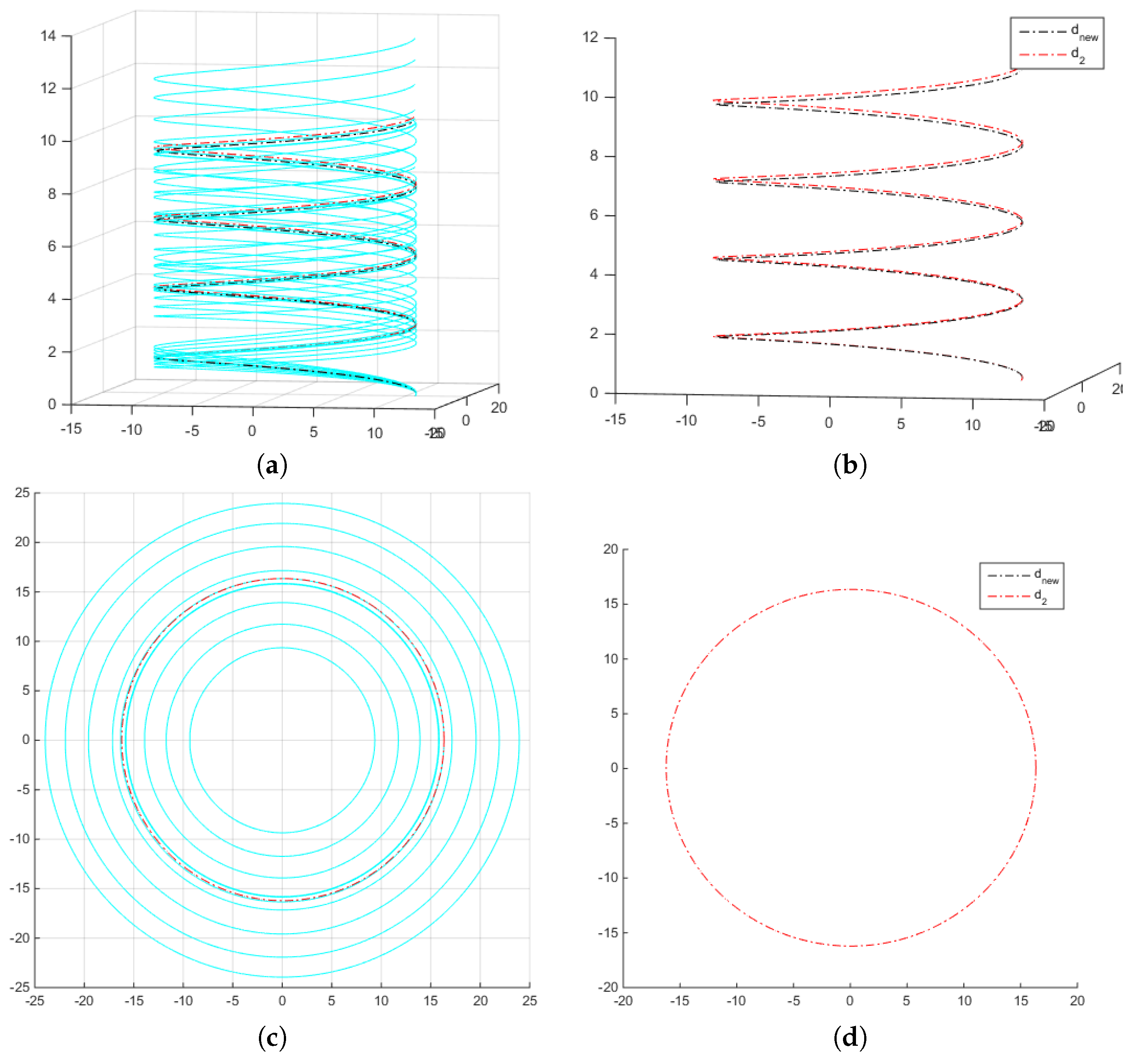
The Karcher means of the ten spirals and of the ten circumferences are computed with the new metric (${\widehat{\beta }}_{new}$, Equation (18)) and by using the distance proposed by [5] in the shape and size space ${\mathcal{S}}_2$. These means are shown in Figure 2, where the original curves are plotted in light blue; ${\widehat{\beta }}_{new}$ is plotted in black color and ${\widehat{\beta }}_2$, the Karcher-mean using the distance $d_2$, is plotted in red color. As can be seen, in Figure 2a,b, there is a very slight difference between the means ${\widehat{\mu }}_{new}$ and ${\widehat{\mu }}_2$ of the ten spirals. Figure 2c,d show that the means coincide in the case of the circumferences.

An example comparing the geodesics obtained with $d_{new}$ and $d_2$, can be seen in Figure 3, without great differences among them.

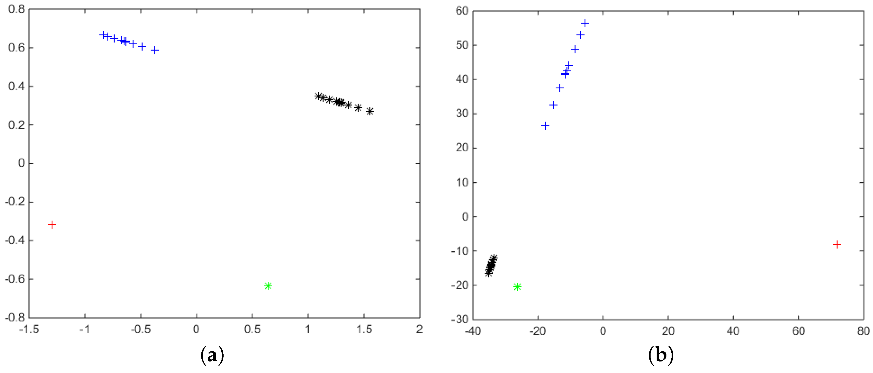
Finally, the distance matrices $D_{new}$ and $D_2$ between the twenty curves are computed using both metrics, and in order to compare the performance of $d_2$ and $d_{new}$, a multidimensional scaling (MDS) analysis [13] has been carried out. The MDS algorithm is a descriptive data reduction procedure to display the information contained in a $(m\times m)$-distance matrix, D, in a low-dimensional space such that the between-object distances are preserved as well as possible. Then, for each distance matrix D, the method looks for a set of orthogonal variables $\{y_1,\cdots ,y_p\}$, $p<m$ such that the Euclidean distances of the elements with respect to these variables are as close as possible to the distances given in the original matrix D. In Figure 4, MDS has been applied to the distance matrices computed with both metrics. In both graphics (Figure 4a,b), the black points represent the twenty spirals ${\alpha }_{1i}$ shown in Figure 1a, and the green points represent the twenty circumferences ${\alpha }_{2i}$ shown in Figure 1b.

As can be seen, there are slights differences among the MDS representations of both metrics. If we perform a k-means cluster with k = 2 from $D_{new}$ and $D_2$, in both cases the two groups are perfectly recovered. We also recover the two groups if we apply DBSCAN [14,15].

If we re-scale the twenty figures, multiplying them by 50, and we consider the twenty resulting curves jointly to the twenty original ones, we can compute again the distance matrices $D_{new}$ and $D_2$ between the 40 curves. The MDS scaling representation of these distance matrices can be found in Figure 5. In both graphics, the initial spirals ${\{{\beta }_{i1}\}}_{i=1,\cdots ,10}$ are plotted in green; the circumferences ${\{{\beta }_{i2}\}}_{i=1,\cdots ,10}$ are plotted in black, and their scaled versions, ${\{50{\beta }_{i1}\}}_{i=1,\cdots ,10}$ and ${\{50{\beta }_{i2}\}}_{i=1,\cdots ,10}$ are plotted in red and blue color, respectively.

Figure 5 shows one important difference between the performance of both metrics. By definition, $d_{new}$ is invariant to changes of scale i.e., $d_{new}({\beta }_{il},{\beta }_{jm})=d_{new}(k{\beta }_{il},k{\beta }_{jm})$, $\forall k\in \mathbb{R}$ and this equality does not hold for $d_2$, where the distance among curves increases with the scaling factor.

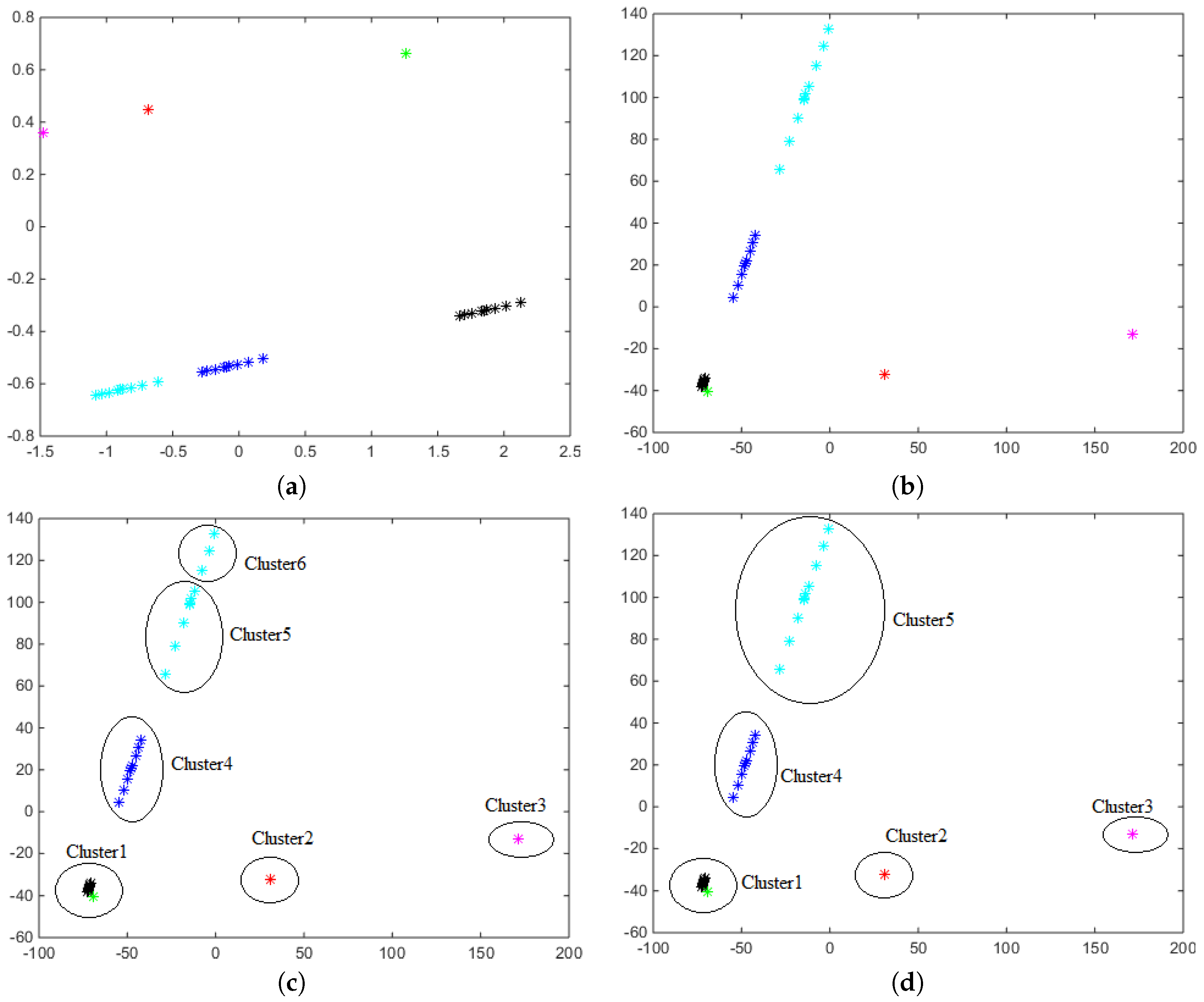
If we perform a k-means cluster analysis with k = 4 from the distance matrices, the four groups are recovered from $D_{new}$, but for $D_2$, the distance among the scaled circumferences increases regarding to the distance among the initial circumferences, so the group of large circumferences is splitted into two clusters while the initial (short) curves (spirals and circumferences) are joined in a unique cluster (Figure 6). However, the algorithm DBSCAN applied on both distance matrices, allow us in both cases recover again the four initial groups.

As a third step of the simulation study, let us consider a broader data set with the initial spirals ${\{{\beta }_{i1}\}}_{i=1,\cdots ,10}$, the circumferences ${\{{\beta }_{i2}\}}_{i=1,\cdots ,10}$, their scaled versions ${\{50{\beta }_{i1}\}}_{i=1,\cdots ,10}$ and ${\{50{\beta }_{i2}\}}_{i=1,\cdots ,10}$, jointly with two new re-scaled sets ${\{250{\beta }_{i1}\}}_{i=1,\cdots ,10}$ and ${\{250{\beta }_{i2}\}}_{i=1,\cdots ,10}$. The distance matrices $D_{new}$ and $D_2$ between the 60 curves are computed and the MDS scaling representation of these distance matrices can be found in Figure 7.

A k-means cluster analysis with $k=6$ so as the DBSCAN algorithm applied on $D_{new}$ recovers the 6 simulated groups. However, the DBSCAN algorithm applied on $D_2$ provides 5 clusters on this data set joining in a single cluster the initial (short) curves (spirals and circumferences) and distinguishing the other groups (Figure 7d). The k-means algorithm with $k=5$ provides the same result, but if the k-means algorithm is applied with $k=6$ clusters, the set of the largest circumferences is split into two groups (Figure 7c). Once again, it can be clearly seen that the distance $d_2$ among shapes increases with the scaling factor.

7. Detection of Outliers

Although there are a variety of techniques for outlier detection for different types of data in any metric space based on nearest-neighbor techniques (see [16] for a detailed explanation), they have not been fully exploited in the shape and size space of curves. Some of the main references are based on box-plots of the distances to the median to detect outliers, such as [12,17], and more recently the method based on elastic depths proposed by [18].

We propose a technique for outlier detection based on the proposed distance. Nearest-neighbor techniques are very popular due to their good results, conceptual simplicity and interpretability in the classic multivariate case [19]. We consider this idea for the shape and size space of curves. The k-NN Anomaly Detection algorithm searches for the nearest k-neighbors, i.e., the k closest curves, for every element in the database, and calculates the average distance of the k-neighbors. In the multivariate case, the Euclidean distance is used, but here we use the proposed distance to find the neighbors. This procedure returns outlier scores; as usual, the highest score denotes the highest degree of outlierness. A way to establish a binary decision about whether or not to label a point as an outlier is to use a box-plot with the outlier scores and to consider the points detected as outliers by the box-plot as anomalies.

We compare our procedure with that introduced in [12,17,18] using the data sets of open curves used in [12,17], which are available from [20]. For the Example 1 considered in [17] formed by 70 spirals, Ref. [12] found 6 outliers, Ref. [17] also found 6 outliers (2 scale outliers and 4 mild shape outliers) and [18] found 4 outliers (3 due to amplitude and 1 due to phase) with the recommended value of k = 2, which is the boxplot multiplier, while 9 outliers are found with the classical k = 1.5. However, with our methodology, we detect 8 outliers (the results are stable, we obtain the same outliers with k = 5, 10 or 15). We have also computed the square of the distance in Equation (17) ($\mathrm{d}{(p,q)}^2$) and we have computed the contribution in percentage due to shape ${\mathrm{d}}_{{\mathcal{C}}^0}^2(\pi \left(p\right),\pi \left(q\right))/\mathrm{d}{(p,q)}^2$ and due to size ${\mathrm{d}}_{\mathbb{R}}^2(lnR\left(p\right),lnR\left(q\right))/\mathrm{d}{(p,q)}^2$, for each outlier. The percentages of contribution due to shape for the 8 outliers are: 21%, 29%, 34%, 35%, 41%, 50%, 50% and 74%. For the Example 3 in [17] formed by 176 fiber tracts in the human brain extracted from a diffusion tensor magnetic resonance image (DT-MRI), we detect the same 11 outliers also detected by [12,17], and all are due to shape, with percentages of contribution due to shape of 90%. However, [18] with k = 2 returned 62 outliers (62 due to amplitude, 23 of them are also outliers due to phase), i.e., 35% of points of the sample are considered outliers.

8. Application to a Real Data Set

Footwear design relies greatly on knowledge of foot size and shape. Proper fit is an essential condition for potential shoe buyers, besides the fact that poorly fitting footwear can cause foot pain and deformity, especially in women. Although people with extreme feet (very different from the rest) may be the most likely customers with poor fit, in anthropometric studies they are not usually searched. However, outliers report very valuable information for the footwear design process, since they can help shoe designers adjust their designs to a larger part of the population and can increase their awareness of customers characteristics that will make them uncomfortable to wear, whether when considering a range of special sizes or modifying any shoe feature to fit more users.

The aim of this section was to detect the outliers in an anthropometric foot database. We carry out a separate analysis for men and women, since gender foot shape differences are well-known [21,22]. Furthermore, footwear designers usually propose different types of shoes for women and men.

8.1. Foot Database

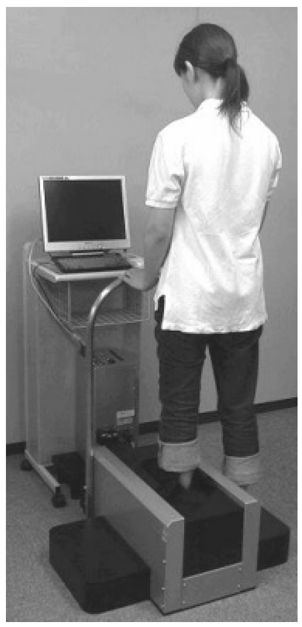
A total of 770 3D right foot scans were carried out. A total of 389 men and 381 women representing the Spanish adult female and male population were measured. The data were collected in different regions across Spain at shoe shops and workplaces using an INFOOT laser scanner [23]. The scanning process is carried out while the participant stands upright placing equal weight on each foot, in a specific position and orientation (see Figure 8). The result is a 3D point cloud representing the complete outer surface of the foot, including the sole of the foot.

3D foot shapes were registered using the method described by [24] with a template made up of 5000 vertices, with five foot landmarks (i.e., 1st and 2nd toe tips; 1st and 5th metatarsal heads; and pternion; see Figure 9). This set of landmarks is automatically located on 3D foot scans and allows the extraction of foot measurements and contours, according to the definitions used by the Human Shape Lab of the Biomechanics Institute of Valencia (IBV), which comply with standards and are compatible with the accepted definitions found in the literature [25,26,27,28]. In particular, we consider the longitudinal contour passing through the Ball Position. The mean shapes for men and women in ${\mathcal{S}}_2$ are displayed in Figure 10.

8.2. Detection of Foot Outliers

We have applied our outlier procedure to the curves of men and women with k = 10. A total of 24 and 18 outliers are detected for men and women, respectively. In order to briefly describe the outlier curves detected, we show the percentiles of each outlier for the four variables that could most influence shoe fit according to shoe design experts. Specifically, these variables are: Foot Length, FL (distance between the rear and foremost point the foot axis); Ball Girth, BG (perimeter of the ball section); Ball Width, BW (maximal distance between the extreme points of the ball section projected onto the ground plane); and Instep Height, IH (maximal height of the instep section, located at 50% of the foot length).

Table 1. Percentile profiles of outliers of foot shape variables for women.

FL	BG	BW	IH
64	44	70	84
36	90	61	65
25	39	17	24
61	95	100	100
66	57	83	70
28	35	73	53
70	58	100	99
66	49	76	46
63	47	79	88
69	88	67	94
48	50	84	64
79	66	23	22
42	54	45	11
73	40	68	35
100	99	68	98
43	4	41	23
30	31	32	13
57	17	35	77

and

Table 2. Percentile profiles of outliers of foot shape variables for men.

FL	BG	BW	IH
69	51	45	53
65	49	38	77
25	39	17	24
75	17	24	14
37	25	60	37
86	74	2	13
47	85	15	21
58	32	3	11
43	59	11	1
72	39	31	48
10	2	8	4
99	78	43	43
7	30	30	82
56	30	12	2
82	39	40	28
20	7	11	54
96	58	53	28
42	54	44	11
53	80	91	100
53	58	28	49
88	72	38	84
3	3	86	79
19	54	84	97
13	37	99	91

show the percentile profiles of the outliers found for women and men, respectively. Note that for some of the outliers some of the variables show extreme percentiles, i.e., very high or very low percentiles. However, in many other cases, outliers do not show extreme values in these variables. Therefore, outliers can be due to the particular combination of the variables or due to the particular configuration of the curve that cannot be summarized by these four variables. In summary, with the proposed procedure, we can detect feet that are “not normal”, which may not be detected with a classic multivariate analysis. Figure 11 shows the most outlier feet for men and women. For men, the outlier feet are the 14th and 9th, while for the women the outliers are the 7th and 17th. Note that those feet do not have really extreme percentiles.

We have also computed the contributions of shape and size. The main contribution is due to shape for both men and women. The mean is 96% for men and 97% for women.

9. Conclusions

We have proposed a new metric in the shape and size space ${\mathcal{S}}_2$ that, unlike the previous proposals, allows us to distinguish whether the distance between two shapes $\left[q_1\right]$ and $\left[q_2\right]$ is due to the difference in shape or to the difference in size between the corresponding curves ${\beta }_1$ and ${\beta }_2$. It has been compared with the metric proposed by [5] in a simulation study, where our proposal is shown to perform better. Furthermore, we also show the advantages of the new metric, such as its invariance to changes of scale.

For the first time, we have also proposed a procedure based on the distances and NN techniques in ${\mathcal{S}}_2$ for finding outlier curves in ${\mathcal{S}}_2$. We have applied it to a novel industrial data set. The foot outliers found by considering their contour can help shoe designers improve their designs in order to provide customers with a better fit.

In future work, in regards to the theory, closed curves could be considered and an the appropriate metric defined. Furthermore, the new metric could be used in other types of statistical problems besides outlier detection, such as classification, clustering, or new ones, where curves in ${\mathcal{S}}_2$ have never been used before, such as archetype analysis [29] or archetypoid analysis [30]. Finally, in regards to the footwear application, the outlier procedure with the new metric could be applied to other kinds of foot contours, such as the Ball Girth, and of course, scopes for other fields of application.

References

1. Dryden, I.; Mardia, K. Size and shape analysis of landmark data. Biometrika 1992, 79, 57–68. [Google Scholar] [CrossRef]
2. Klassen, E.; Srivastava, A.; Mio, M.; Joshi, S.H. Analysis of planar shapes using geodesic paths on shape spaces. IEEE Trans. Pattern Anal. Mach. Intell. 2004, 26, 372–383. [Google Scholar] [CrossRef] [PubMed]
3. Younes, L.; Michor, P.; Shah, J.; Mumford, D. A Metric on Shape Space With Explicit Geodesics. Rend. Lincei Mat. Appl. 2008, 19, 25–57. [Google Scholar] [CrossRef] [Green Version]
4. Srivastava, A.; Klassen, E.; Joshi, S.H.; Jermyn, I.H. Shape analysis of elastic curves in euclidean spaces. IEEE Trans. Pattern Anal. Mach. Intell. 2011, 33, 1415–1428. [Google Scholar] [CrossRef] [PubMed] [Green Version]
5. Kurtek, S.; Srivastava, A.; Klassen, E.; Ding, Z. Statistical Modeling of Curves Using Shapes and Related Features. J. Am. Stat. Assoc. 2012, 107, 1152–1165. [Google Scholar] [CrossRef]
6. Sundaramoorthi, G.; Mennucci, A.; Soatto, S.; Yezzi, A. A new geometric metric in the space of curves, and applications to tracking deforming objects by prediction and filtering. SIAM J. Imaging Sci. 2011, 4, 109–145. [Google Scholar]
7. Kouchi, M. 3—Anthropometric methods for apparel design: Body measurement devices and techniques. In Anthropometry, Apparel Sizing and Design; Gupta, D., Zakaria, N., Eds.; Woodhead Publishing: Cambridge, UK, 2014; pp. 67–94. [Google Scholar]
8. Kuehnapfel, A.; Ahnert, P.; Loeffler, M.; Broda, A.; Scholz, M. Reliability of 3D laser-based anthropometry and comparison with classical anthropometry. Sci. Rep. 2016, 6, 26672. [Google Scholar] [CrossRef] [PubMed] [Green Version]
9. Srivastava, A.; Klassen, E.P. Functional and Shape Data Analysis; Springer: Berlin/Heidelberg, Germany, 2016. [Google Scholar]
10. Pennec, X. Intrinsic Statistics on Riemannian Manifolds: Basic Tools for Geometric Measurements. J. Math. Imaging Vis. 2006, 25, 127–154. [Google Scholar] [CrossRef] [Green Version]
11. Le, H. Locating Fréchet means with application to shape spaces. Adv. Appl. Probab. 2001, 33, 324–338. [Google Scholar] [CrossRef]
12. Kurtek, S.; Su, J.; Grimm, C.; Vaughan, M.; Sowell, R.; Srivastava, A. Statistical analysis of manual segmentations of structures in medical images. Comput. Vis. Image Underst. 2013, 117, 1036–1050. [Google Scholar] [CrossRef]
13. Cox, T.F.; Cox, M.A. Multidimensional Scaling; CRC Press: Boca Raton, FL, USA, 2000. [Google Scholar]
14. Ester, M.; Kriegel, H.P.; Sander, J.; Xu, X. A density-based algorithm for discovering clusters in large spatial databases with noise. In Proceedings of the Kdd, Portland, OR, USA, 2–4 August 1996; Volume 96, pp. 226–231. [Google Scholar]
15. Hahsler, M.; Piekenbrock, M.; Doran, D. dbscan: Fast density-based clustering with R. J. Stat. Softw. 2019, 91, 1–30. [Google Scholar] [CrossRef] [Green Version]
16. Aggarwal, C.C. Outlier Analysis, 2nd ed.; Springer: Berlin/Heidelberg, Germany, 2017. [Google Scholar]
17. Xie, W.; Chkrebtii, O.; Kurtek, S. Visualization and Outlier Detection for Multivariate Elastic Curve Data. IEEE Trans. Vis. Comput. Graph. 2019. [Google Scholar] [CrossRef]
18. Harris, T.; Tucker, J.D.; Li, B.; Shand, L. Elastic depths for detecting shape anomalies in functional data. Technometrics 2020, 1–25. [Google Scholar] [CrossRef]
19. Goldstein, M.; Uchida, S. A comparative evaluation of unsupervised anomaly detection algorithms for multivariate data. PLoS ONE 2016, 11, e0152173. [Google Scholar] [CrossRef] [PubMed] [Green Version]
20. Cho, M.H.; Asiaee, A.; Kurtek, S. Elastic Statistical Shape Analysis of Biological Structures with Case Studies: A Tutorial. Bull. Math. Biol. 2019, 81, 2052–2073. [Google Scholar] [CrossRef] [PubMed]
21. Krauss, I.; Langbein, C.; Horstmann, T.; Grau, S. Sex-related differences in foot shape of adult Caucasians—A follow-up study focusing on long and short feet. Ergonomics 2011, 54, 294–300. [Google Scholar] [CrossRef] [PubMed]
22. Saghazadeh, M.; Kitano, N.; Okura, T. Gender differences of foot characteristics in older Japanese adults using a 3D foot scanner. J. Foot Ankle Res. 2015, 8, 29. [Google Scholar] [CrossRef] [PubMed] [Green Version]
23. I-Ware Laboratory. Available online: http://www.i-ware.co.jp/ (accessed on 24 August 2020).
24. Allen, B.; Curless, B.; Popović, Z. The space of human body shapes: Reconstruction and parameterization from range scans. ACM Trans. Graph. (TOG) 2003, 22, 587–594. [Google Scholar] [CrossRef]
25. Rossi, W.A.; Tennant, R. Professional Shoe Fitting; National Shoe Retailers Association: Bicester, UK, 2013. [Google Scholar]
26. Ramiro, J.; Alcántara, E.; Forner, A.; Ferrandis, R.; García-Belenguer, A.; Durá, J.; Vera, P.; Brizuela, G.; Llana, S. Guía de Recomendaciones Para el Diseño de Calzado; Instituto de Biomecánica de Valencia: Valencia, Spain, 1995; pp. 135–151. [Google Scholar]
27. Goonetilleke, R.S. The Science of Footwear; CRC Press: Boca Raton, FL, USA, 2012. [Google Scholar]
28. Luximon, A. Handbook of Footwear Design and Manufacture; Elsevier: Amsterdam, The Netherlands, 2013. [Google Scholar]
29. Cutler, A.; Breiman, L. Archetypal Analysis. Technometrics 1994, 36, 338–347. [Google Scholar] [CrossRef]
30. Vinué, G.; Epifanio, I.; Alemany, S. Archetypoids: A new approach to define representative archetypal data. Comput. Stat. Data Anal. 2015, 87, 102–115. [Google Scholar]
Figure 1. Simulated curves. (a) Ten spirals with different shapes and common length. (b) Ten circumferences with common shape and different lengths.
Mathematics 08 01691 g001
Figure 2. (a,c) Simulated curves and their corresponding means. (b,d) Comparison of the Karcher means obtained with the two different distances.
Mathematics 08 01691 g002
Figure 3. Comparison of the geodesic obtained using the two different distances.
Mathematics 08 01691 g003
Figure 4. Multidimensional scaling (MDS) applied to the distance matrices: (a) using d n e w , (b) using d 2 . The ten spirals are marked in green and the ten circumferences are represented with black asterisks.
Mathematics 08 01691 g004
Figure 5. MDS applied to the distance matrices: (a) using d n e w , (b) using d 2 . The ten initial spirals are marked in green and the ten initial circumferences are represented with black asterisk, the spirals re-scaled by 50 are the red asterisks and the circumferences are plotted in blue.
Mathematics 08 01691 g005
Figure 6. MDS applied to the distance matrices: (a) using d n e w , (b) using d 2 . The ten initial spirals are marked with green asterisks and the ten initial circumferences are represented with black asterisks, the enlarged spirals are plotted in red and the enlarged circumferences are plotted in blue.
Mathematics 08 01691 g006
Figure 7. MDS applied to the distance matrices: (a) using d n e w , (b) using d 2 . The ten initial spirals are marked in green and the ten initial circumferences are represented with black asterisks. The enlarged spirals are plotted in red (factor 50) and magenta (factor 250) and the enlarged circumferences are plotted in blue (factor 50) and cyan (factor 250). The clusters obtained on d 2 are plotted: (c) using k-means algorithm with k = 6 , (d) using DBSCAN and k-means, k = 5 .
Mathematics 08 01691 g007
Figure 8. Infoot® scanner.
Mathematics 08 01691 g008
Figure 9. Foot landmarks used for registration in the database and foot template topology (the last image).
Mathematics 08 01691 g009
Figure 10. Mean shapes of contours for men (left) and women (right).
Mathematics 08 01691 g010
Figure 11. The most outlier feet for men (first row) and women (second row).
Mathematics 08 01691 g011