Define
as a column vector which consists of a basis of holomorphic differentials on
M. Up to exact one-forms, the Abelian differentials of the second kind are given by
and we set
. Let
be a canonical homology basis on
M. We shall determine a complex
matrix given by
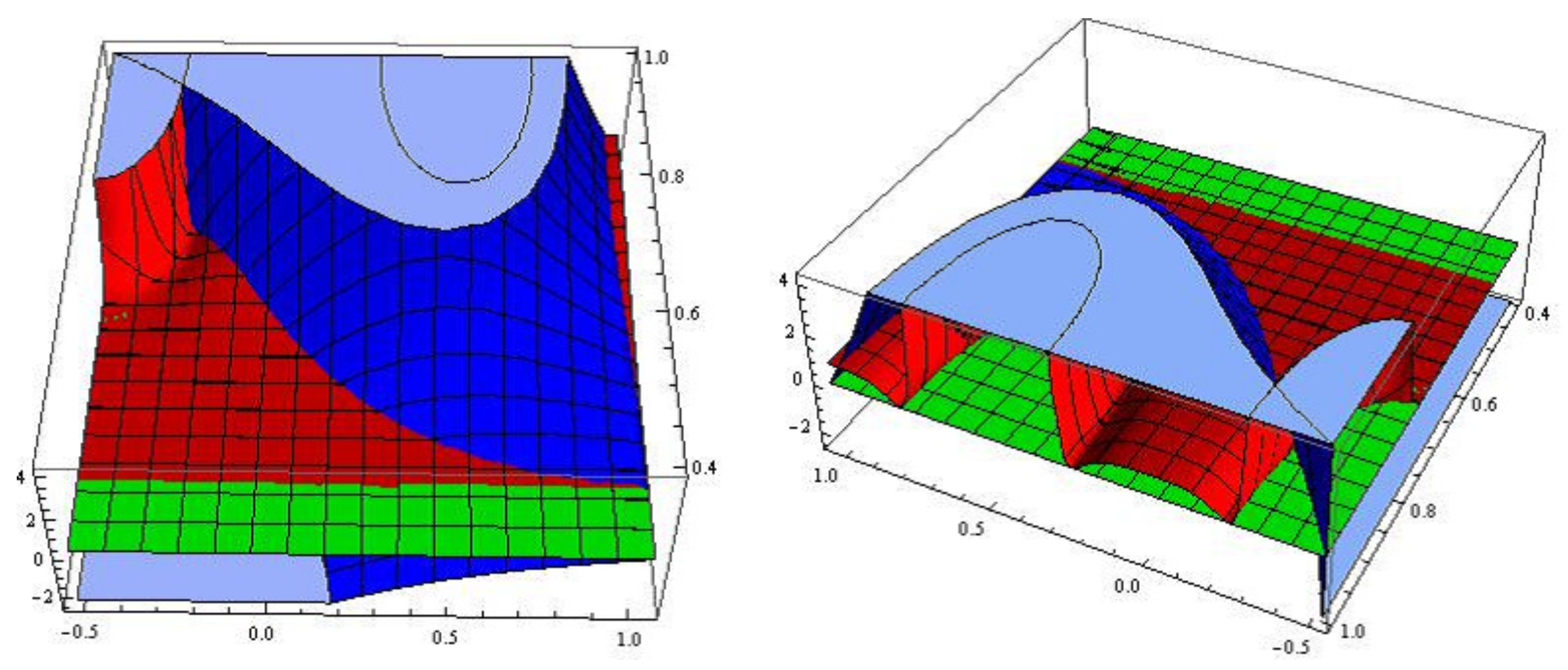
We now construct
M as a two-sheeted branched cover of
. Let
be the two-sheeted covering defined by
which is branched at the following eight fixed points of
j:
Figure A1.
M represented as a two-sheeted branched cover of .
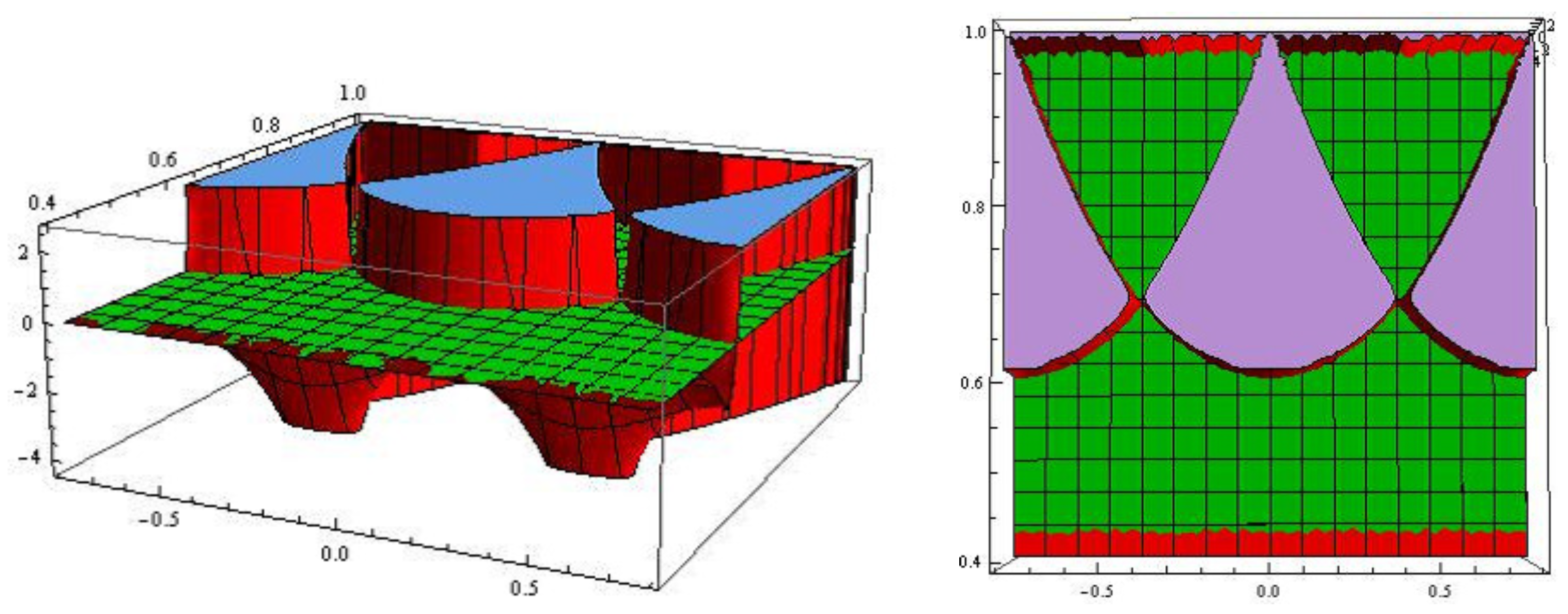
Figure A2.
The action of j on M.
Appendix A.1.1. A Canonical Homology Basis
We first take the following three key paths.
where we choose the branches as follows:
and
for
.
and
for
. For
,
.
Remark A2. Straightforward calculations yield For , we have . For , holds. For , we find . Hence , , have single-valued branches for .
We now consider two cases, namely, the case
and the case
. We assume
, and introduce the following two paths.
where we choose the branches as follows:
and
for
.
and
for
.
Using
and
, we shall describe a canonical homology basis on
M by
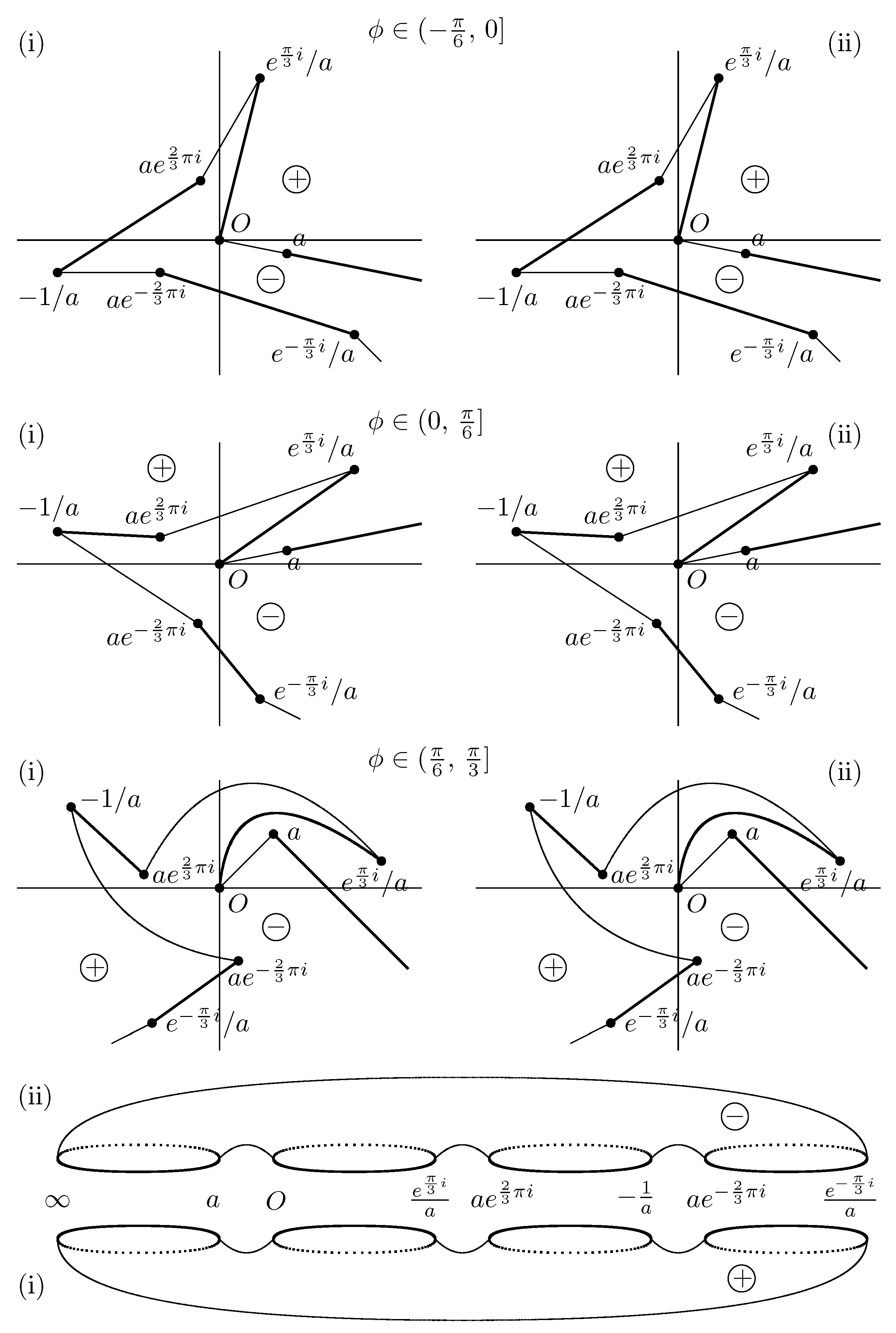
. To start with, let us choose
as in
Figure A3.
There exist
such that
is homologous to
(write
) for an arbitrary
. Setting
, we have
(see § 5.2.1 in [
8]). Thus,
hold for
(see
Figure A4). In the process we have also shown that the equation
is satisfied for
.
By choosing a suitable
, we find
. From
, we have
Setting
, we obtain
. It follows that
holds for
(see
Figure A5).
Figure A4.
, , in (i).
Figure A4.
, , in (i).
By
,
, and (
A2),
for
. Combining (
A1) and (
A4), we have
for
.
Similarly, there exists
such that
. From
and (
A5), we find
(see
Figure A6).
Figure A6.
, , in (i).
Figure A6.
, , in (i).
By
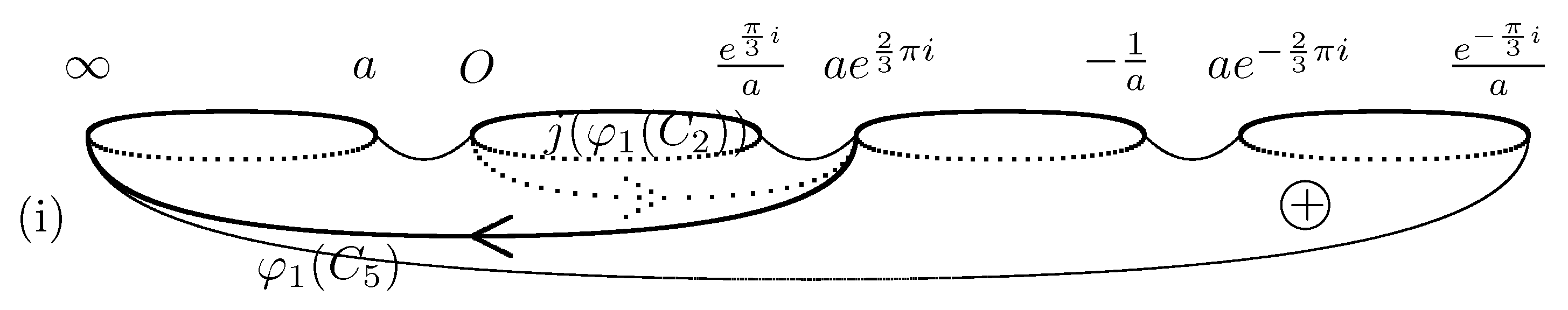
, we obtain
(see
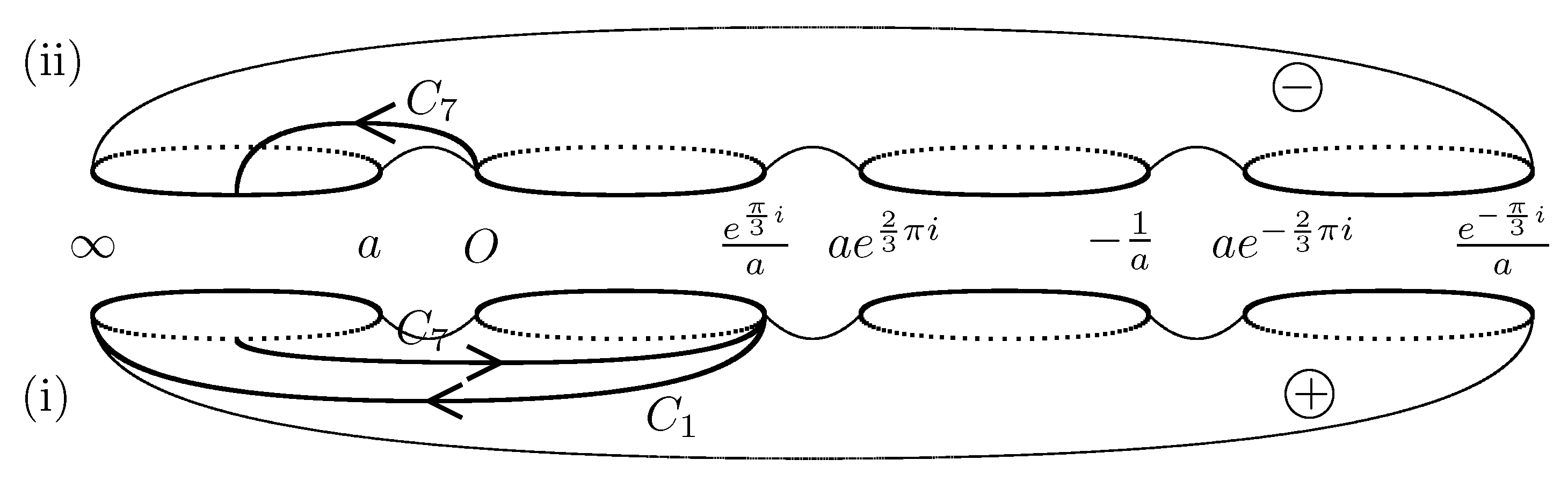
Figure A7).
Figure A7.
, in (i).
Figure A7.
, in (i).
Choosing suitable
, we have
. From
and (
A5), we find
,
(see
Figure A8).
Figure A8.
, in (i).
Figure A8.
, in (i).
To determine
and
, we introduce the following new path.
where we choose the branch such that
.
Remark A3. Thus, holds for and we may choose the branch such that . Substituting , we have , where .
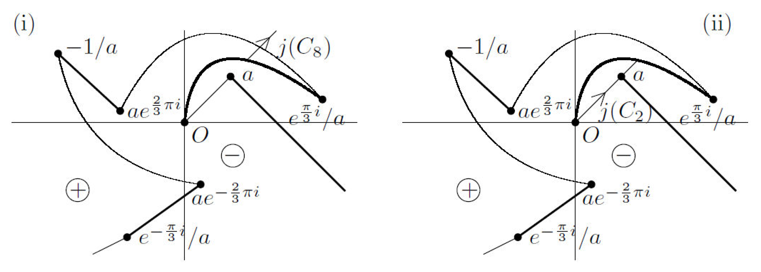
By Remark A3,
holds. Substituting
to
in
, we find
. Hence
(see
Figure A9 and
Figure A10).
Figure A10.
, in M.
Figure A10.
, in M.
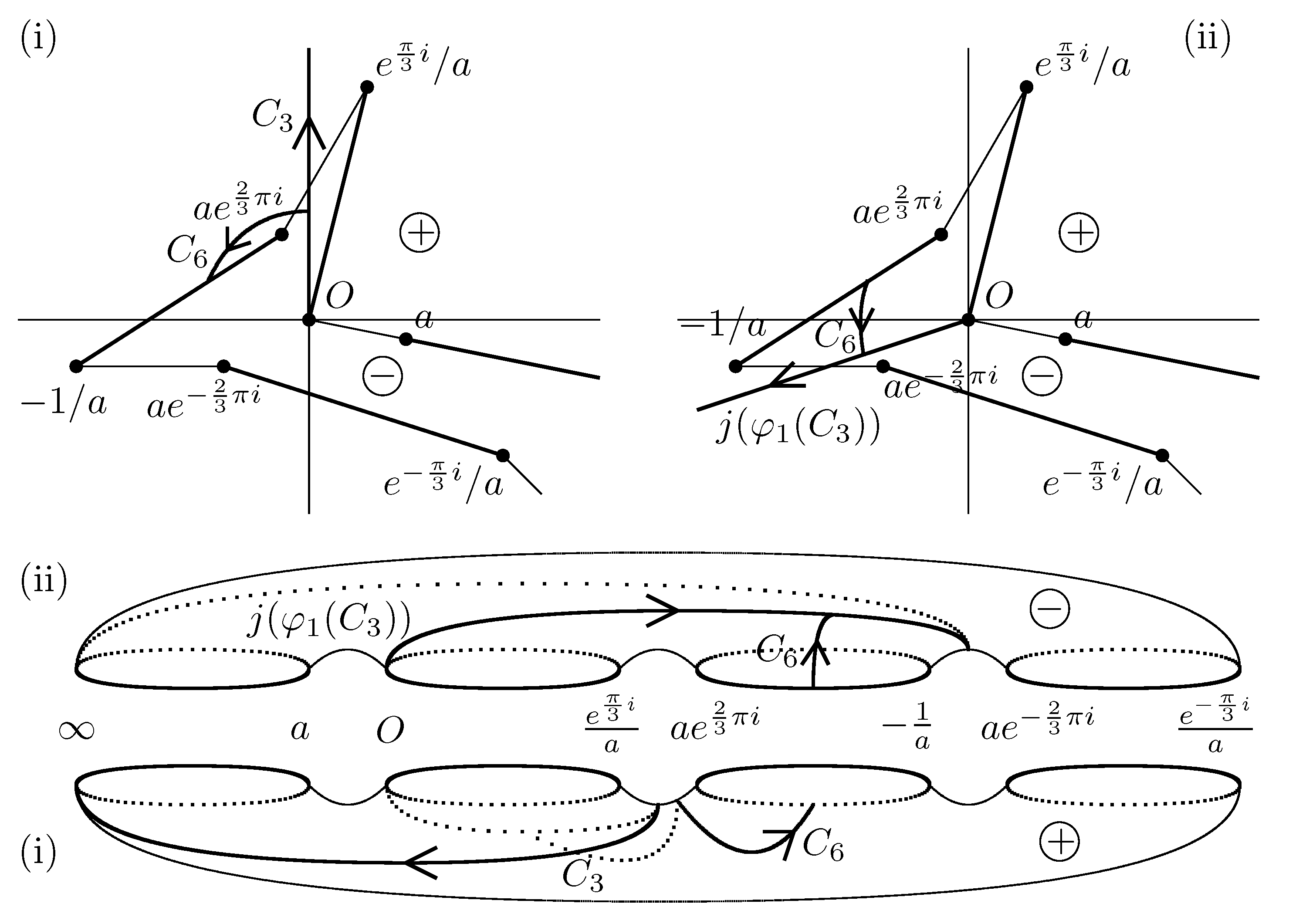
By
, we obtain
, and so
Figure A11 follows.
Figure A11.
, in (i).
Figure A11.
, in (i).
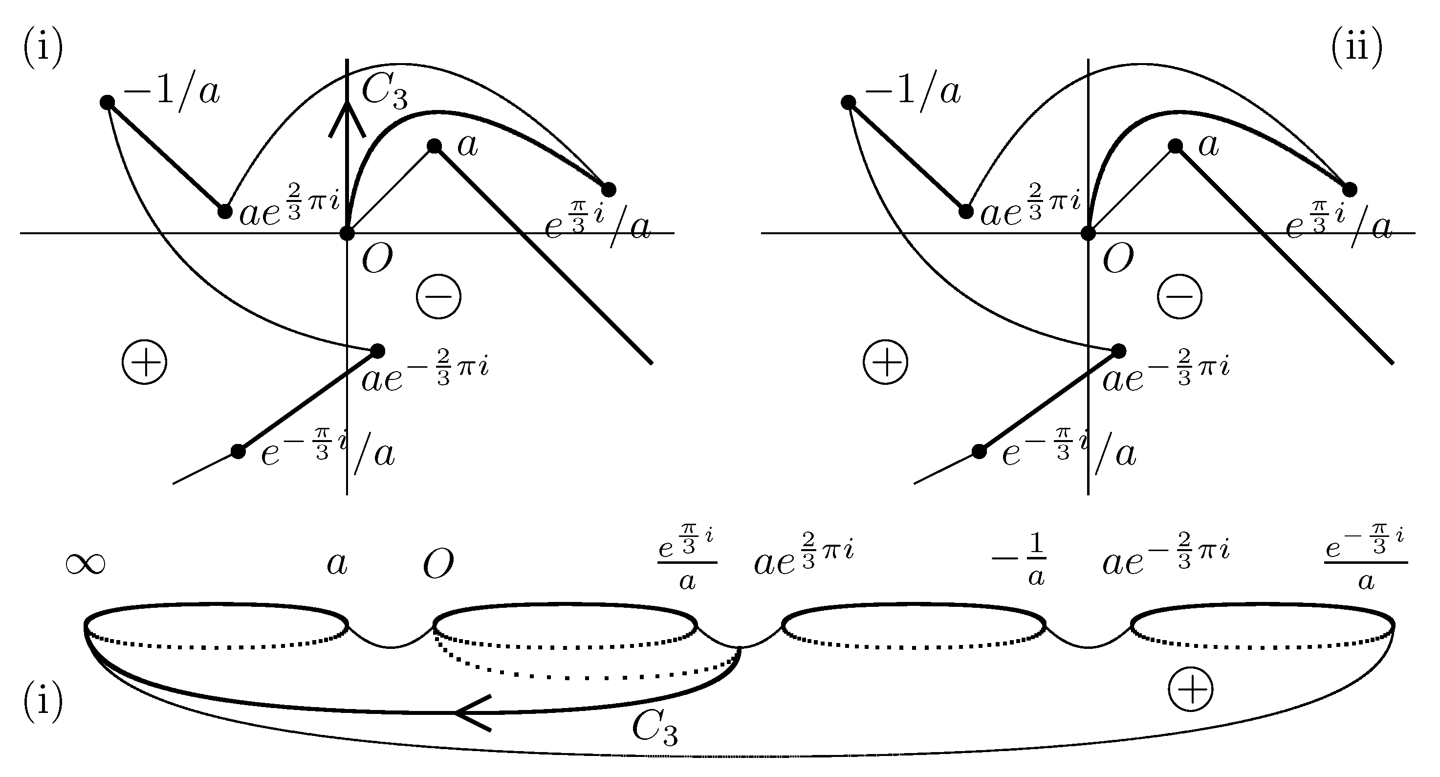
From
, we have
(see
Figure A12).
Figure A12.
, in (i).
Figure A12.
, in (i).
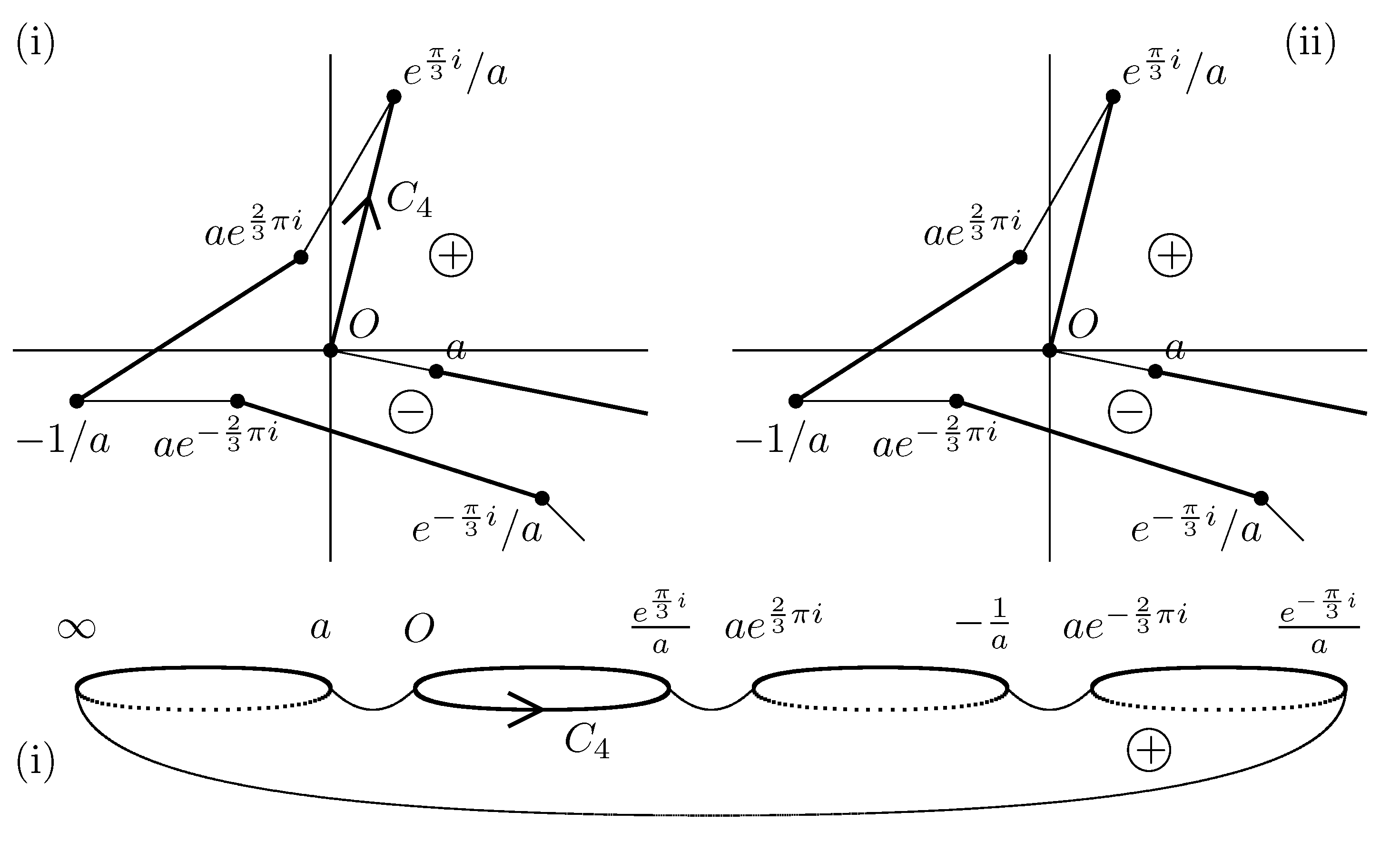
Therefore, we can describe a canonical homology basis as follows (see
Figure A13).
Figure A13.
A canonical homology basis on M.
Figure A13.
A canonical homology basis on M.
Next we assume
, and introduce the following two paths.
where we choose the branches as follows:
and
for
.
and
for
.
Using
and
, we shall describe a canonical homology basis on
M by
. To start with, let us choose
as in
Figure A14.
There exist
such that
. So we find
that is,
Setting
, we have
(see
Figure A15).
Figure A15.
, in M.
Figure A15.
, in M.
By
, we find
From
, we have
To determine
, we introduce the following path.
where we choose the branch such that
.
Remark A4. Thus, holds for and we may choose the branch such that . Substituting , we have , where .
By Remark A4,
holds. Substituting
to
in
, we find
. Hence
(see
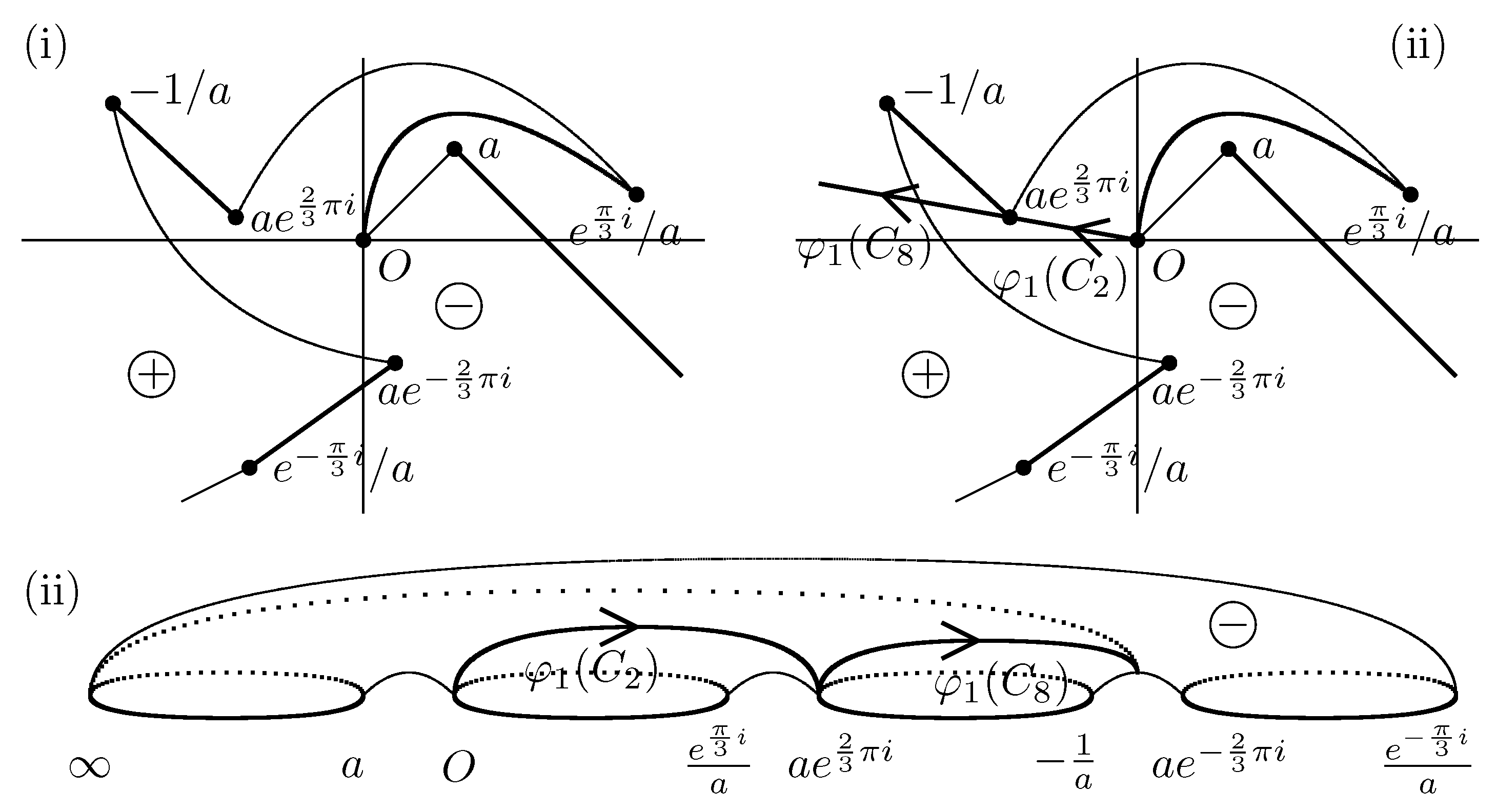
Figure A16).
Figure A16.
, in M.
Figure A16.
, in M.
From
, we have
(see
Figure A17).
Figure A17.
, in (ii).
Figure A17.
, in (ii).
Choosing suitable
, we obtain
. By
and (
A8), we find
(see
Figure A20).
Figure A18.
, in (ii).
Figure A18.
, in (ii).
By similar arguments as
, we obtain
and
(see
Figure A19).
Figure A19.
, in M.
Figure A19.
, in M.
From
, we have
(see
Figure A20).
Figure A20.
, in M.
Figure A20.
, in M.
Therefore, we can obtain the same canonical homology basis as for
(see
Figure A13).
Finally, by
Figure A15 and
Figure A20, we find
. Combining (
A10) and
implies


