Estimation and Prediction of Record Values Using Pivotal Quantities and Copulas

Abstract

Recently, the area of sea ice is rapidly decreasing due to global warming, and since the Arctic sea ice has a great impact on climate change, interest in this is increasing very much all over the world. In fact, the area of sea ice reached a record low in September 2012 after satellite observations began in late 1979. In addition, in early 2018, the glacier on the northern coast of Greenland began to collapse. If we are interested in record values of sea ice area, modeling relationships of these values and predicting future record values can be a very important issue because the record values that consist of larger or smaller values than the preceding observations are very closely related to each other. The relationship between the record values can be modeled based on the pivotal quantity and canonical and drawable vine copulas, and the relationship is called a dependence structure. In addition, predictions for future record values can be solved in a very concise way based on the pivotal quantity. To accomplish that, this article proposes an approach to model the dependence structure between record values based on the canonical and drawable vine. To do this, unknown parameters of a probability distribution need to be estimated first, and the pivotal-based method is provided. In the pivotal-based estimation, a new algorithm to deal with a nuisance parameter is proposed. This method allows one to reduce computational complexity when constructing exact confidence intervals of functions with unknown parameters. This method not only reduces computational complexity when constructing exact confidence intervals of functions with unknown parameters, but is also very useful for obtaining the replicated data needed to model the dependence structure based on canonical and drawable vine. In addition, prediction methods for future record values are proposed with the pivotal quantity, and we compared them with a time series forecasting method in real data analysis. The validity of the proposed methods was examined through Monte Carlo simulations and analysis for Arctic sea ice data.

1. Introduction

Extreme weather and air pollution have been received steadily increasing attention over the past decade. Examples include extreme temperatures, the exceedances of flood peaks, and pollutant concentrations deviating considerably from expected average levels. In such cases, predicting observations more extreme than the current extreme values is an important issue. The topic of record values was introduced by Chandler [1], and Balakrishnan et al. [2] established some recurrence relationships for single and double moments of lower record values from the Gumbel distribution. Coles and Tawn [3] analyzed a daily rainfall series for modeling the extremes of a rainfall process in the context of the record values. Wang et al. [4] provided approaches to constructing exact confidence intervals (CIs) for unknown parameters in the family of proportional reversed hazard distributions based on lower record values. Seo and Kim [5] provided classical and Bayesian approaches to inference for the Gumbel distribution based on lower record values. Seo and Kim [6] presented an objective Bayesian analysis method for the two-parameter Rayleigh distribution based on record values. Seo and Kim [7] proposed an entropy inference method based on an objective Bayesian approach for when observed record values have a two-parameter logistic distribution.

There are two types of the record values. If the observation is greater than all the preceding observations it is called the upper record. On the other hand, if the observation is smaller than all the preceding observations then it is called the lower record. There are a few situations where lower record values are of special interest. For example, Arctic sea ice greatly affects climate change, and the reduction of Arctic sea ice is a very serious issue. In this case, only sea ice extent less than the previous one is of interest and recorded, which poses a problem of predicting the next sea ice extent. The lower record value is described as follows. Let $\left\{X_1,X_2,\dots \right\}$ be a sequence of independent and identically distributed (iid) random variables with a probability density function (PDF) $f\left(x\right)$ and a cumulative distribution function (CDF) $F\left(x\right)$. Then, $X_j$ is a lower record value if $X_j<X_i$ for every $i<j.$ The indexes for which lower record values occur are given by the record times $\left\{L\left(k\right),k\ge 1\right\}$, where $L\left(k\right)=\min \left\{j|j>L(k-1),X_j<X_{L(k-1)},\right\},k>1,$ with $L\left(1\right)=1.$ Therefore, a sequence of lower record values is denoted by $\left\{X_{L\left(k\right)},k=1,2,\dots \right\}$ from the original sequence $\left\{X_1,X_2,\dots \right\}.$ These record values are heavily related to each other. Imani and Braga-Neto [8] proposed an efficient finite-horizon feedback controller similar to an optimal linear quadratic Gaussian estimator for partially-observed Boolean dynamical systems as a general class of nonlinear state-space model. Imani et al. [9] proposed an optimal Bayesian filter approach to the problem of recursive estimation in partially-observed Boolean dynamical systems. To establish the relationship between the record values, a copulas approach based on the canonical (C) and drawable (D) vine is proposed in this article.

Copulas have recently received much attention as a modeling tool for describing the dependency structure of multivariate data. The notion of a copula function can be found in Sklar [10]. One of the advantages of copula models is to build a variety of dependence structures based on existing parametric or non-parametric models of the marginal distributions. The copulas can be described as follows. Let F be the d-dimensional function of the random vector $\mathit{X}={(X_1,\dots ,X_d)}^T$ with marginal distributions $F_{X_1}\left(x\right),\dots ,F_{X_d}\left(x\right)$. Then there exists a copula C such that for all $\mathit{x}={(x_1,\dots ,x_d)}^T\in {[-\infty ,\infty ]}^d$,

$$\begin{array}{c}\hfill F\left(\mathbf{x}\right)=C\left(F_{X_1}\left(x\right),\dots ,F_{X_d}\left(x\right)\right),\end{array}$$

where the copula C is unique if $F_{X_1}\left(x\right),\dots ,F_{X_d}\left(x\right)$ are continuous by Sklar’s theorem (Sklar [10], 1959). In this case, the copula C can be interpreted as the distribution function of a d-dimensional random variable on ${[0,1]}^d$ with uniform marginal distributions. Tsung et al. [11] conducted a comprehensive literature review of statistical transfer learning methods focusing on statistical models and statistical methodologies, including a Gaussian copula. Rocher et al. [12] proposed a generative copula-based method that can elaborately estimate the likelihood that a particular person will be correctly re-identified, even in a very incomplete dataset. Vine copulas were introduced by Joe [13] to overcome limitations of standard multivariate copulas in higher dimensions, where standard multivariate copulas lack the flexibility of accurately modeling the dependence.

Aas et al. [14] described statistical inference techniques for the C- and D-vine copulas. Berg and Aas [15] and Fischer et al. [16] showed the excellence of the D-vine copula approach, compared to alternative copulas in constructing higher dimensional dependency structures.

To the best of our knowledge, modeling the dependence structure between record values numerically has been little explored. In this paper, we propose an approach with which to model the relationship between the record values based on C- and D-vine copulas and to predict future record values.

The remainder of the article is organized as follows. Section 2 introduces C- and D-vine copulas and provides pivotal-based approaches to estimate the model parameters and to predict future record values by proposing a new algorithm to deal with a nuisance parameter. Section 3 presents simulation studies to validate the proposed approaches. We applied the methods to Arctic sea ice data; see Section 4. Concluding remarks and some discussions are in Section 5.

2. Methods

Let $f\left(x;\theta \right)$ and $F\left(x;\theta \right)$ be the marginal density and distribution functions of X, respectively, where $\theta$ is an unknown parameter. Then a schematic diagram (Figure 1) of our method is given by

Figure 1. Schematic diagram.

The C -and D-vine copulas are first described in the following subsection.

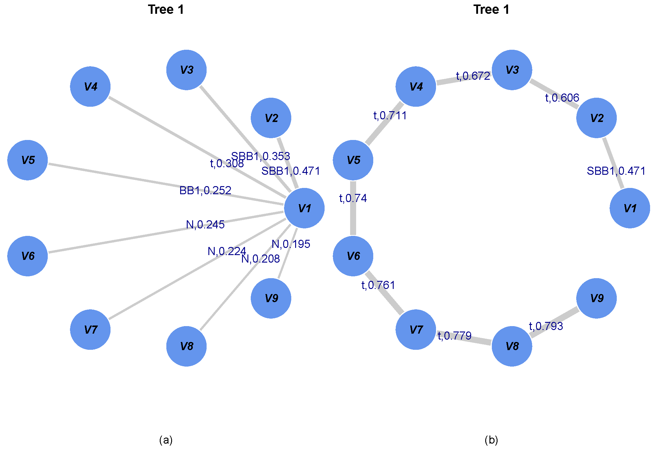
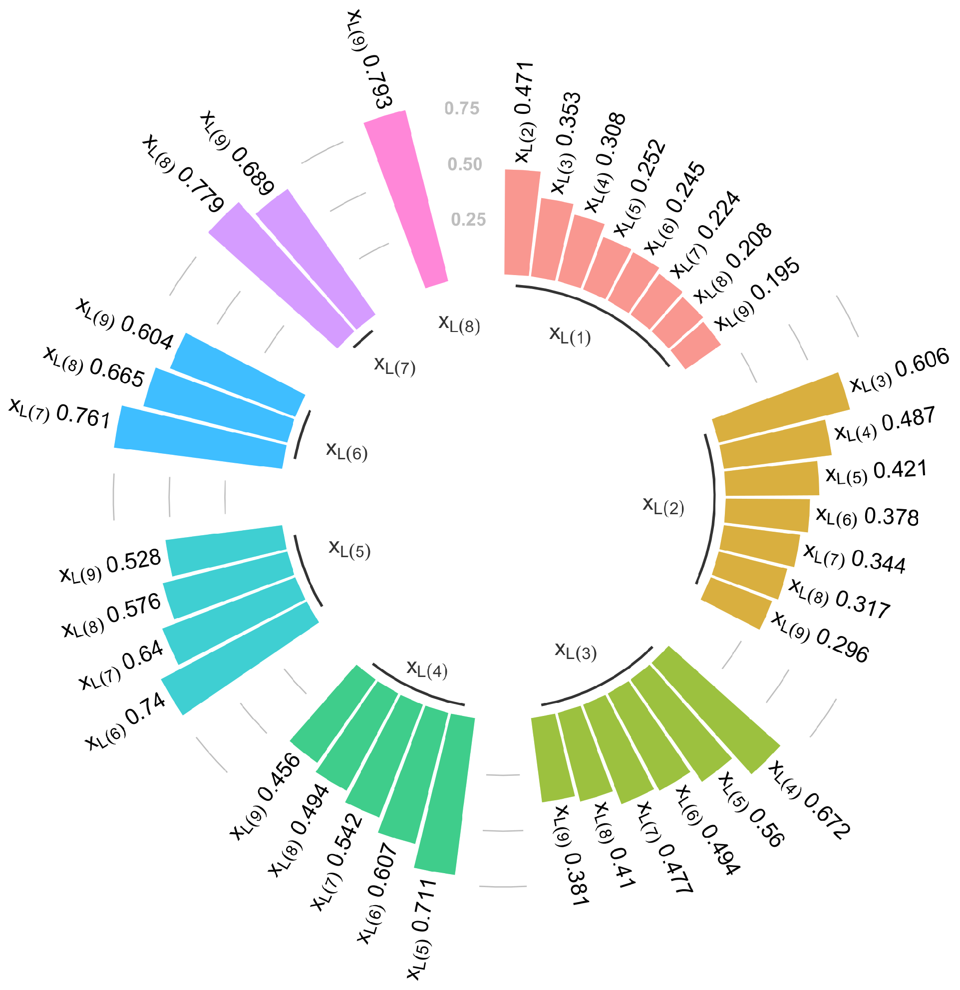
2.1. C- and D-Vine Copulas

A vine is a flexible graphical model that decomposes a multivariate probability distribution into bivariate copulas, where each pair-copula can be chosen independently from the others [14]. This article considers C- and D-vine copulas to model the relationship between record values based on C- and D-vine copulas.

The C-vine decomposition is given by

$$\begin{array}{cc}\hfill f(x_1,\dots ,x_n)& =f_1\left(x_1\right)\prod _{i=2}^n\prod _{k=1}^{i-1}{c}_{i-k,i|1,\dots ,x_{i-k-1}}{f}_k\left(x_i\right)\hfill \\ \hfill & =\prod _{k=1}^n{f}_k\left(x_k\right)\left(\prod _{j=1}^n\prod _{i=1}^{k-1}{c}_{i-k,i|1,\dots ,i-k-1}\right)\hfill \\ \hfill & =\prod _{k=1}^n{f}_k\left(x_k\right)\left(\prod _{j=1}^{n-1}\prod _{i=1}^{n-j}{c}_{j,j+i|1,\dots ,j-1}\right).\hfill \end{array}$$

Then, we can specify the pairs of the d-dimensional C-vine copula model in the following order:

$$\begin{array}{ccc}\hfill & (1,2),(1,3),(1,4),\dots ,(1,d),\hfill & \left(\mathrm{tree}1\right)\hfill \\ \hfill & (2,3|1),(2,4\left|1\right),\dots ,(2,d|1),\hfill & \left(\mathrm{tree}2\right)\hfill \\ \hfill & \cdots ,\hfill \\ \hfill & (d-1,d|1,\dots ,d-2).\hfill & (\mathrm{tree}d-1),\hfill \end{array}$$

which has vectors of length $d(d-1)/2$, where d is the number of variables.

The D-vine decomposition is given by

$$\begin{array}{cc}\hfill f(x_1,\dots ,x_n)& =\prod _{i=2}^n{f}_{i|x_1,\dots ,x_{i-1}}\left(x_i\right)f_1\left(x_1\right)\hfill \\ \hfill & =\prod _{l=1}^n{f}_l\left(x_l\right)\left(\prod _{i=2}^n\prod _{j=1}^{i-2}{c}_{ji|j+1,\dots ,i-1}\right)\prod _{i=2}^n{c}_{i-1,i}\hfill \\ \hfill & =\prod _{l=1}^n{f}_l\left(x_l\right)\left(\prod _{i=2}^{n-1}\prod _{j=1}^{n-i}{c}_{j,i|j+1,\dots ,j+i-1}\right).\hfill \end{array}$$

Similarly, the pairs of the d-dimensional D-vine copula model are specified in the following order:

$$\begin{array}{ccc}\hfill & (1,2),(2,3),(3,4),\dots ,(d-1,d),\hfill & \left(\mathrm{tree}1\right)\hfill \\ \hfill & (1,3|2),(2,4\left|3\right),\dots ,(d-2,d|d-1),\hfill & \left(\mathrm{tree}2\right)\hfill \\ \hfill & (1,4|2,3),(2,5|3,4),\dots ,(d-3,d|d-2,d-1),\hfill & \left(\mathrm{tree}3\right)\hfill \\ \hfill & \cdots ,\hfill \\ \hfill & (1,d|2,\dots ,d-1).\hfill & (\mathrm{tree}d-1)\hfill \end{array}$$

To measure the dependence of each pair-copula, we consider tree 1 that can be employed to obtain Kendall’s $\tau$ (Nelsen [17], 2006) given by

$$\begin{array}{cc}\hfill {\tau }_C& =4\left({\int }_0^1{\int }_0^{1}C(u_i,u_j)dC(u_i,u_j)\right)-1\hfill \\ \hfill & =4E\left[C(U_i,U_j)\right]-1,\hfill \end{array}$$

where $C(u_i,u_j)$ is a bivariate copula function for $u_i,u_j\in [0,1]$.

In a C- and D-vine, consider the exponentiated Gumbel distribution (EGD) with the CDF

$$\begin{array}{c}\hfill F\left(x\right)={\left(e^{-e^{-x/\sigma }}\right)}^{\lambda },-\infty <x<\infty ,\sigma ,\lambda >0,\end{array}$$

(1)

where $\sigma$ and $\lambda$ are the scale and shape parameters. Then, $u_i$ is the value of the marginal distribution of $X_{L\left(i\right)}$ with

$$\begin{array}{c}\hfill F_{X_{L\left(i\right)}}\left(x\right)=e^{-H\left(x\right)}\sum _{j=0}^{i-1}\frac{{\left[H\left(x\right)\right]}^j}{j!},\end{array}$$

(2)

where $H\left(x\right)=-logF\left(x\right)$ (Ahsanullah [18] and Arnold et al. [19]). That is, for $d-1$ pairs of data points $\{(x_{L\left(i\right)},x_{L\left(j\right)});i<j\}$, the corresponding couples $\{(u_i,u_j);i<j\}$ can be computed from the marginal distribution (2). In addition, the marginal density function of $X_{L\left(i\right)}$ is given by

$$\begin{array}{c}\hfill f_{X_{L\left(i\right)}}\left(x\right)=\frac{1}{\Gamma \left(k\right)}{\left[-logF\left(x\right)\right]}^{i-1}f\left(x\right).\end{array}$$

Note that it is necessary to estimate $\sigma$ and $\lambda$ for computing the values of $u_i$ and $u_j$.

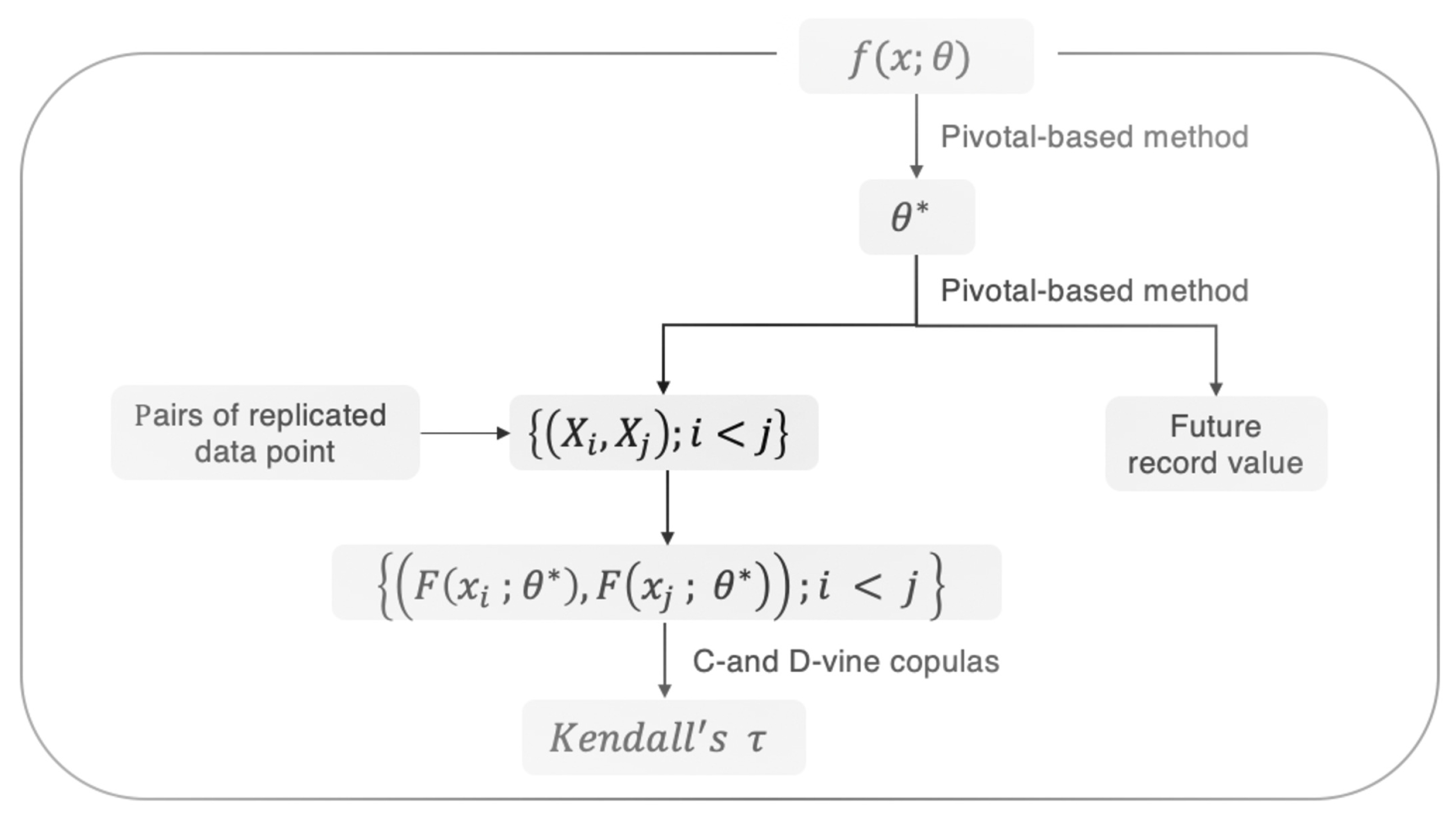
2.2. Pivotal-Based Approach

Here we present a pivotal-based method to estimate the parameters of the CDF (1). First, a lemma is introduced to deal with nuisance parameters in order to establish the relationship between record values.

Lemma 1.

Let $X_{L\left(1\right)},\cdots ,X_{L\left(k\right)}$ be the lower record values from the CDF (1). Then,

(a) 

$T_k(\sigma ,\lambda )=2\lambda e^{-X_{L\left(k\right)}/\sigma }$ has a ${\chi }^2$ distribution with $2k$ degrees of freedom;

(b) 

$V\left(\sigma \right)=\frac{e^{(X_{L\left(1\right)}-X_{L\left(k\right)})/\sigma }-1}{k-1}$ has a F distribution with $2k-2$ and 2 degrees of freedom;

(c) 

$W\left(\sigma \right)=\frac{2\left({\sum }_{j=1}^k{X}_{L\left(j\right)}-k{X}_{L\left(k\right)}\right)}{\sigma }$ has a ${\chi }^2$ distribution with $2k-2$ degrees of freedom.

Proof. 

Let $X_{L\left(1\right)},\cdots ,X_{L\left(k\right)}$ be the lower record values from the CDF (1). Then, we have

$$\begin{array}{c}\hfill Z_i=-logF\left(x_{L\left(i\right)}\right),i=1,\dots ,k\end{array}$$

that have a standard exponential distribution, and that leads to the following spacings

$$\begin{array}{cc}\hfill S_i& =Z_i-Z_{i-1},i=1,\dots ,k(Z_0\equiv 0),\hfill \end{array}$$

which is independent and identically distributed as the standard exponential distribution with mean 1. From the spacings, the pivotal quantities

$$\begin{array}{cc}\hfill T_j(\sigma ,\lambda )& =2\sum _{i=1}^j{S}_i\hfill \\ \hfill & =2\lambda e^{-X_{L\left(j\right)}/\sigma },j=1,\dots ,k\hfill \end{array}$$

(3)

are derived, which are independent random variables such that there is an ${\chi }^2$ distribution with $2j(j=1,\dots ,k)$. From (3), the pivotal quantity (a) is easily proved. In addition, let $T_{-1,k}(\sigma ,\lambda )=2{\sum }_{i=2}^k{S}_i$. Then, the pivotal quantity (b) is proved as

$$\begin{array}{cc}\hfill V\left(\sigma \right)& =\frac{T_{-1,k}(\sigma ,\lambda )/(2k-2)}{T_1(\sigma ,\lambda )/2}\hfill \\ \hfill & =\frac{e^{(X_{L\left(1\right)}-X_{L\left(k\right)})/\sigma }-1}{k-1}\hfill \end{array}$$

because $T_{-1,k}(\sigma ,\lambda )$ and $T_1(\sigma ,\lambda )$ are independent random variables, given the fact that $S_i\left(i=1,\dots ,k\right)$ are independent and identically random values, as mentioned earlier; both have a ${\chi }^2$ distribution with $2k-2$ and 2 degrees of freedom, respectively. On top of that, we can derive the following pivotal quantities by using Lemma 2 of Wang et al. [4] in (3)

$$\begin{array}{cc}\hfill U_j& ={\left(\frac{T_j(\sigma ,\lambda )}{T_{j+1}(\sigma ,\lambda )}\right)}^j\hfill \\ \hfill & =e^{j(X_{L(j+1)}-X_{L\left(j\right)})/\sigma },j=1,\dots ,k-1\hfill \end{array}$$

which are independent and identically distributed as the uniform distribution on the interval $(0,1)$. Then, the pivotal quantity (c) is proved as

$$\begin{array}{cc}\hfill W\left(\sigma \right)& =-2\sum _{j=1}^{k-1}log{U}_j\hfill \\ \hfill & =\frac{2\left({\sum }_{j=1}^k{X}_{L\left(j\right)}-k{X}_{L\left(k\right)}\right)}{\sigma }.\hfill \end{array}$$

☐

From Lemma 1(c), the unique solution ${\sigma }^{*}$ is given by

$$\begin{array}{c}\hfill {\sigma }^{*}=\frac{2\left({\sum }_{j=1}^k{X}_{L\left(j\right)}-k{X}_{L\left(k\right)}\right)}{Q_W},\end{array}$$

where $Q_W$ follows a ${\chi }^2$ distribution with $2k-2$ degrees of freedom. Then, for any $0<\alpha <1$, an exact $100(1-\alpha )\%$ CI for $\sigma$ based on $W\left(\sigma \right)$ is given by

$$\begin{array}{c}\hfill \left({\sigma }_{\left(\right[(\alpha /2)N\left]\right)}^{*},{\sigma }_{\left(\right[(1-\alpha /2)N\left]\right)}^{*}\right),\end{array}$$

where ${\sigma }_{\left(\right[\alpha N\left]\right)}$ is the $\left[\alpha N\right]$th smallest of $\left\{{\sigma }_l^{*}\right\}$. Note that the exact CI is the equal-tail CI because it splits the probability equally, putting $\alpha /2$ in each tail of the distribution. For any $0<\alpha <1$, an exact $100(1-\alpha )\%$ CI with the shortest-length based on ${\sigma }^{*}$ is given by

$$\begin{array}{c}\hfill \left({\sigma }_{\left(l^{*}\right)}^{*},{\sigma }_{\left(l^{*}+\left[(1-\alpha )N\right]\right)}^{*}\right),\end{array}$$

where $l^{*}$ is chosen so that

$$\begin{array}{c}\hfill {\sigma }_{\left(l^{*}+\left[(1-\alpha )N\right]\right)}^{*}-{\sigma }_{\left(l^{*}\right)}^{*}=\underset{1\le l\le N-\left[\right(1-\alpha \left)N\right]}{min}\left[{\sigma }_{\left(l+\left[\right(1-\alpha \left)N\right]\right)}^{*}-{\sigma }_{\left(l\right)}^{*}\right].\end{array}$$

Similarly, the unique solution from $V\left(\sigma \right)$ in Lemma 1 is given by

$$\begin{array}{c}\hfill {\sigma }^{*}=\frac{X_{L\left(1\right)}-X_{L\left(k\right)}}{log\left[1+(k-1)Q_F\right]},\end{array}$$

where $Q_F$ follows a F distribution with $2k-2$ and 2 degrees of freedom. Then, with the same argument, the exact $100(1-\alpha )\%$ equal-tailed and shortest CIs for $\sigma$ based on $V\left(\sigma \right)$ can be constructed. In Section 3, it is found that $W\left(\sigma \right)$ provides a more efficient CI than $V\left(\sigma \right)$ in terms of average lengths (ALs) of the CIs through Monte Carlo simulations, as in the case of Seo and Kim [5].

For $\lambda$, we have that

$$\begin{array}{c}\hfill \lambda =\frac{T_k}{2e^{-X_{L\left(k\right)}/\sigma }}\end{array}$$

(4)

by putting $T_k=T_k(\sigma ,\lambda )$ in Lemma 1. In addition, let $g(W,{\mathit{x}}_{\mathit{L}})$ be the unique solution of $W\left(\sigma \right)=W$ for $W>0$, where ${\mathit{x}}_{\mathit{L}}=\left(x_{L\left(1\right)},\cdots ,x_{L\left(k\right)}\right)$. Then, by substituting $g(W,{\mathit{x}}_{\mathit{L}})$ for $\sigma$ in (4), the following generalized quantity is given by

$$\begin{array}{c}\hfill \psi =\frac{T_k}{2e^{-X_{L\left(k\right)}/g(W,{\mathit{x}}_{\mathit{L}})}}.\end{array}$$

The existing literature (Wang et al. [4] and Wang et al. [20]) supposed that W has a ${\chi }^2$ distribution with $2k-2$ degrees of freedom, and then obtained the percentiles of $\psi$ generating W and $T_k$ independently from the ${\chi }^2$ distribution with $2k-2$ and $2k$ degrees of freedom, respectively, althrough W and $T_k$ are not independent. As an alternative, the following algorithm is proposed to obtain the percentiles of $\psi$.

Step 1.

Generate $Q_{{\chi }^2,1},Q_{{\chi }^2,2},\dots ,Q_{{\chi }^2,k}$ from a ${\chi }^2$ distribution with two degrees of freedom.

Step 2.

Compute $T_j={\sum }_{i=1}^j{Q}_{{\chi }^2,i}$ for $i=1,\dots ,k$.

Step 3.

Compute $W=2{\sum }_{j=1}^{k-1}log\left(\frac{T_k}{T_j}\right)$ and solve the equation $W\left(\sigma \right)=W$ for $\sigma$ to obtain $g(W,{\mathit{x}}_{\mathit{L}})$.

Step 4.

Compute $\psi$.

Step 5.

Repeat $N(\ge 10,000)$ times.

From the algorithm, the equal-tailed and shortest CIs for $\lambda$ based on $\psi$ are given by

$$\begin{array}{c}\hfill \left({\psi }_{\left(\right[(\alpha /2)N\left]\right)},{\psi }_{\left(\right[(1-\alpha /2)N\left]\right)}\right)\end{array}$$

and

$$\begin{array}{c}\hfill \left({\psi }_{\left(l^{*}\right)},{\psi }_{\left(l^{*}+\left[(1-\alpha )N\right]\right)}\right),\end{array}$$

respectively, where $l^{*}$ is chosen so that

$$\begin{array}{c}\hfill {\psi }_{\left(l^{*}+\left[(1-\alpha )N\right]\right)}-{\psi }_{\left(l^{*}\right)}=\underset{1\le l\le N-\left[\right(1-\alpha \left)N\right]}{min}\left[{\psi }_{\left(l+\left[\right(1-\alpha \left)N\right]\right)}-{\psi }_{\left(l\right)}\right].\end{array}$$

2.3. Prediction

Let $X_{L\left(r\right)}(r=k+1,k+2,\cdots )$ be the future lower record values. Then, for any $0<\alpha <1$, the conditional quantile is given by

$$\begin{array}{cc}\hfill X_{L\left(r\right),\alpha }\mid x_{L\left(k\right)}& =F_{X_{L\left(r\right)}|X_{L\left(k\right)}}^{-1}\left(\alpha \right)\hfill \\ \hfill & =inf\{y\in \mathbb{R}|F_{X_{L\left(r\right)}|X_{L\left(k\right)}}\left(y\right)\ge \alpha \},\hfill \end{array}$$

where $F_{X_{L\left(r\right)}|x_{L\left(k\right)}}(·)$ is the conditional distribution of $X_{L\left(r\right)}$ given $x_{L\left(k\right)}$. However, the quantile cannot be obtained numerically because it does not have closed forms. Instead, we propose a pivotal approach based on the following lemma.

Lemma 2.

Let $Y_C=logF\left(x_{L\left(k\right)}\right)-logF\left(x\right)$ in the conditional density function of $X_{L\left(r\right)}$ given $x_{L\left(k\right)}$ be defined by Ahsanullah [18] as

$$\begin{array}{c}\hfill f_{X_{L\left(r\right)}|x_{L\left(k\right)}}\left(x\right)=\frac{{\left[logF\left(x_{L\left(k\right)}\right)-logF\left(x\right)\right]}^{r-k-1}f\left(x\right)}{\Gamma (r-k)F\left(x_{L\left(k\right)}\right)},x_{L\left(r\right)}<x_{L\left(k\right)}.\end{array}$$

(5)

Then, $Y_C$ has a gamma distribution with the parameters $(r-k,1)$.

Proof. 

Let $Y_C=logF\left(x_{L\left(k\right)}\right)-logF\left(x\right)$ in (5). Then, the Jacobian of the transformation is

$$\begin{array}{cc}\hfill J& =\frac{\mathrm{d}}{\mathrm{d}{y}_C}x\hfill \\ \hfill & =\frac{F\left(x_{L\left(k\right)}\right)}{f\left(x\right)}{e}^{-y},\hfill \end{array}$$

and the density function of $Y_C$ is

$$\begin{array}{c}\hfill f_{Y_C}\left(y\right)=\frac{1}{\Gamma (r-k)}{y}^{r-k-1}{e}^{-y},\end{array}$$

which is the probability density function of a gamma distribution with parameters $(r-k,1)$. ☐

With the same argument as Section 2, an algorithm for obtaining the Markov-chain Monte-Carlo (MCMC) samples $X_{L\left(r\right)}^i(i=1,\dots ,N)$ based on the pivotal quantity $Y_C$ is provided as follows.

Step 1.

Generate $Y_C$ from Gam$(r-k,1)$.

Step 2.

Compute

$$\begin{array}{c}\hfill X_{L\left(r\right)}\mid x_{L\left(k\right)}=-\sigma log\left(\frac{Y_C}{\lambda }+e^{-x_{L\left(k\right)}/\sigma }\right).\end{array}$$

Step 3.

Repeat steps 1 and 2, N times.

3. Simulation Study

A simulation study was performed to examine the validity of the proposed pivotal-based approach in terms of the coverage probabilities (CPs) and ALs of the proposed confidence intervals (CIs). The lower record values with sizes $k=6\left(2\right)12$ were generated from the standard EGD distribution with $\lambda =0.5,0.8,$ and $1.5$. To construct the $95\%$ exact CIs described in Section 2.2, $N=20,000$ MCMC samples were generated, and the corresponding CPs and average lengths (ALs) were computed over 10,000 simulations. The results are reported in Table 1 along with those for the classical inference (see Proof) (Appendix A) for comparison. Table 1 shows that the CIs using MCMC samples have nearly same results as those using the classical method, and all considered CIs are well matched to their corresponding nominal levels; however, the CIs based on $W\left(\sigma \right)$ have shorter length than those based on $V\left(\sigma \right)$. In addition, all ALs decrease with an increase in the size of record values k. For ALs, the CIs with the shortest-lengths have shorter lengths than those with equal-tails, as expected.

Table 1. Coverage probabilities (CPs) (average lengths (ALs)) of CIs for $\sigma$ and $\lambda$.

		$\mathit{\sigma }$								$\mathit{\lambda }$
		Equal-Tails				Shortest				Equal-Tails	Shortest
		$\mathit{V}\left(\mathbf{\sigma }\right)$		$\mathit{W}\left(\mathbf{\sigma }\right)$		$\mathit{V}\left(\mathbf{\sigma }\right)$		$\mathit{W}\left(\mathbf{\sigma }\right)$		$\mathbf{\psi }$
$\mathbf{\lambda }$	$\mathit{k}$	Classical	MCMC	Classical	MCMC	Classical	MCMC	Classical	MCMC	MCMC
0.5	6	0.948(3.094)	0.948(3.093)	0.950(2.600)	0.949(2.565)	0.951(2.623)	0.950(2.603)	0.952(2.214)	0.950(2.194)	0.950(2.942)	0.942(2.440)
	8	0.949(2.456)	0.948(2.455)	0.950(1.957)	0.949(1.923)	0.951(2.172)	0.949(2.150)	0.951(1.740)	0.949(1.712)	0.954(2.791)	0.946(2.344)
	10	0.948(2.123)	0.948(2.120)	0.950(1.618)	0.949(1.604)	0.950(1.925)	0.947(1.905)	0.952(1.475)	0.950(1.454)	0.952(2.731)	0.947(2.268)
	12	0.948(1.915)	0.948(1.919)	0.948(1.405)	0.948(1.401)	0.951(1.765)	0.948(1.760)	0.949(1.301)	0.948(1.297)	0.950(2.580)	0.944(2.174)
0.8	6	0.948(3.094)	0.948(3.093)	0.950(2.600)	0.949(2.565)	0.951(2.623)	0.950(2.603)	0.952(2.214)	0.950(2.194)	0.950(3.517)	0.942(3.006)
	8	0.949(2.456)	0.948(2.455)	0.951(1.957)	0.949(1.923)	0.951(2.172)	0.949(2.150)	0.951(1.740)	0.949(1.712)	0.953(3.406)	0.944(2.942)
	10	0.948(2.123)	0.948(2.120)	0.950(1.618)	0.949(1.604)	0.950(1.925)	0.947(1.905)	0.952(1.475)	0.950(1.454)	0.954(3.370)	0.948(2.887)
	12	0.948(1.915)	0.948(1.919)	0.948(1.405)	0.948(1.401)	0.951(1.765)	0.948(1.760)	0.949(1.301)	0.948(1.297)	0.950(3.225)	0.940(2.801)
1.5	6	0.948(3.094)	0.948(3.093)	0.950(2.600)	0.949(2.565)	0.951(2.623)	0.950(2.603)	0.952(2.214)	0.950(2.194)	0.950(4.561)	0.940(4.068)
	8	0.949(2.456)	0.948(2.455)	0.951(1.957)	0.949(1.923)	0.951(2.172)	0.949(2.150)	0.951(1.740)	0.949(1.712)	0.953(4.486)	0.945(4.027)
	10	0.948(2.123)	0.948(2.120)	0.950(1.618)	0.949(1.604)	0.950(1.925)	0.947(1.905)	0.952(1.475)	0.950(1.454)	0.957(4.482)	0.943(4.007)
	12	0.948(1.915)	0.948(1.919)	0.948(1.405)	0.948(1.401)	0.951(1.765)	0.948(1.760)	0.949(1.301)	0.948(1.297)	0.952(4.346)	0.939(3.939)

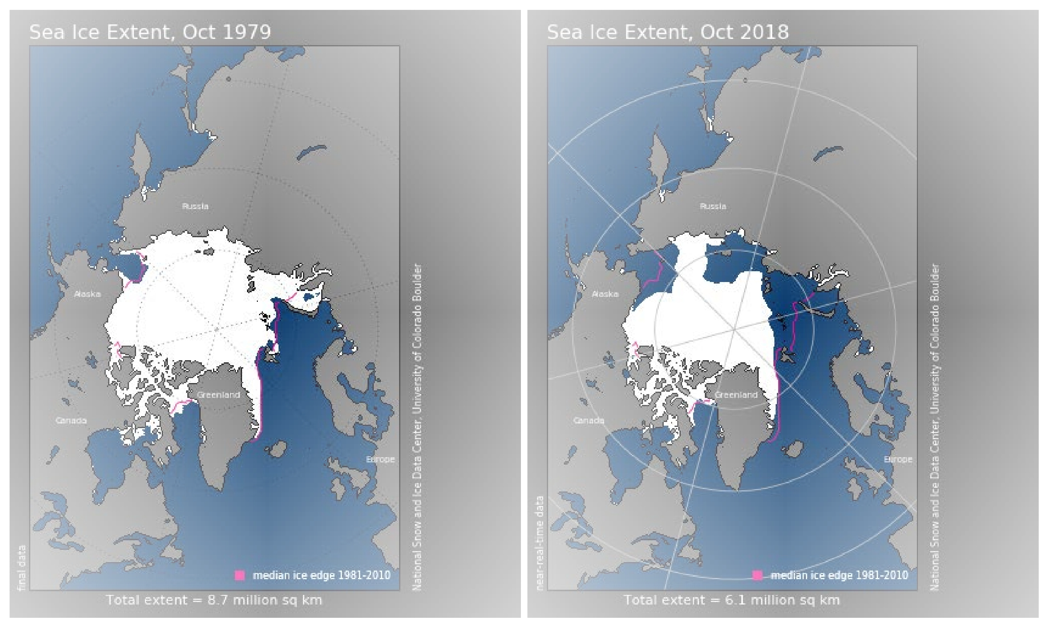
4. Application: Arctic Sea Ice

Sea ice maintains the Earth’s average temperature by reflecting solar energy and keeping the polar regions cool. Currently, the Arctic is warming faster than any other region on earth. The warming of the Arctic Circle leads to a decrease in sea ice, which again causes warming of the Arctic Circle. In addition, it causes global weather changes such as summer heat waves, winter cold waves, and heavy snow. These climate changes are leading to disturbances of ecosystems formed around Arctic sea ice and changes in habitats. For this reason, the importance of sea prediction systems to cope with climate change is increasing. The National Aeronautics and Space Administration (NASA) reported that the area covered by Arctic sea ice has decreased by about ten percent in the last 30 years (Figure 2).

Figure 2. Sea ice extent in October 1979 (left) and October 2018 (right).

This section analyzes the smallest annual Arctic sea ice extent (see Table 2) from October 1978 to October 2018 extracted from the National Snow & Ice Data Center (NSIDC).

Table 2. Observed record values from Arctic sea ice data

i	1	2	3	4	5	6	7	8	9
$x_{L\left(i\right)}$	3.95	2.66	2.47	2.32	2.19	2.17	2.05	1.60	1.29

To measure goodness of fit of the EGD, the replicated data of observed lower record value $x_{L\left(i\right)}$ were generated from its marginal density function with ${\sigma }^{*}$ and $\psi$. All results were obtained by generating $N=50,000$ MCMC samples. In addition, based on the results in the previous simulation study, ${\sigma }^{*}$ from $W\left(\sigma \right)$ was only considered in this data analysis.

The $95\%$ confidence region for the replicated data was plotted in Figure 3. It was found that the confidence regions decreased as the record value of the smallest annual Arctic sea ice decreased. The correlation coefficient between the observed and expected lower record values indicates a strong association.

Figure 3. 95% Confidence region of the replicated data. The solid line represents the mean of the replicated data and r is the correlation coefficient of the mean and observed lower record values.

To examine the relationship between observed record values, Figure 4 plots the first trees of the C- and D-vines with the best copula function in terms of the Akaike information criterion (AIC) and corresponding Kendall $\tau$.

Figure 4. (a) First tree of C-vine for the observed record values; (b) first tree of D-vine for the observed record values. The labels are the best pair-copula families and corresponding Kendall’s $\tau$ values. For example, N, t, BB1, and SBB1 represent Gaussian, Student t, Clayton Gumbel, and survival Clayton Gumbel copula, respectively.

Note that the AIC is defined as $-2ln\left(L\right)+2k$, where L is the likelihood function and k is the number of estimated parameters of the model. Therefore, the smaller the AIC, the better. The entire result for the relationships between observed lower record values is reported in Figure 5. It is shown that the observed lower record values have a positive dependence on each other. In addition, the Kendall’s $\tau$ values increase as the interval between the lower record times decreases. That indicates that $x_{L\left(i\right)}$ and $x_{L\left(j\right)}$ such that $j-i=1$ for $j\ne i$ have the strongest dependency in terms of the Kendall $\tau$. It is worth noting that the strength of dependency between $x_{L\left(i\right)}$ and $x_{L\left(j\right)}$ such that $j-i=1$ for $j\ne i$ becomes stronger as the lower record times increase.

Figure 5. Circular plot for Kendall’s $\tau$ between two paired record values.

The $95\%$ exact CIs for $\sigma$ and $\lambda$ are reported in Table 3, which shows a similar pattern to the simulation results.

Table 3. CIs for $\sigma$ and $\lambda$.

		$\mathit{\sigma }$		$\mathit{\lambda }$
		$\mathit{V}\left(\mathit{\sigma }\right)$	$\mathit{W}\left(\mathit{\sigma }\right)$	$\mathit{W}\left(\mathit{\sigma }\right)$
Equal-tails	Classical	(0.462, 2.672)	(0.631, 2.635)	-
	MCMC	(0.465, 2.675)	(0.631, 2.619)	(9.747, 77.629)
Shortest	Classical	(0.349, 2.330)	(0.526, 2.333)	-
	MCMC	(0.347, 2.321)	(0.507, 2.302)	(6.130, 65.137)

For prediction, the last lower record value $x_{L\left(9\right)}$ was assumed to be unknown, and a time series analysis was conducted, in which it was expected that differences of the observed lower record values could yield a stationary time series because the observed lower record values had a decreasing pattern. In fact, the ARIMA (0, 1, 0) model was chosen as the best model in terms of the AIC from an ARIMA (p, d, q) model, where p is the autoregressive (AR) model order, d is the difference order, and q is the moving average (MA) model order. Table 4 and Figure 6 present the results for future record values of the least annual Arctic sea ice. Table 4 shows that there is little difference in measures of center such as the mean and median for the predictions of the future lower record values based on the pivotal quantity $Y_C$.

Table 4. Prediction results.

	Mean	Median	Equal-Tails	Shortest
$X_{L\left(9\right)}^{*}\mid x_{L\left(8\right)}$	1.457	1.516	(0.987, 1.599)	(1.118, 1.600)
$X_{L\left(9\right)}^{TS}$	1.407	-	(1.071, 1.850)	-
$X_{L\left(10\right)}^{*}\mid x_{L\left(8\right)}$	1.336	1.401	(0.735, 1.583)	(0.876, 1.600)
$X_{L\left(10\right)}^{TS}$	1.237	-	(0.840, 1.821)	-
$X_{L\left(11\right)}^{*}\mid x_{L\left(8\right)}$	1.231	1.298	(0.552, 1.560)	(0.693, 1.591)
$X_{L\left(11\right)}^{TS}$	1.087	-	(0.677, 1.746)	-

Figure 6. Estimated kernel density functions for $X_{L\left(r\right)}^{*}\mid x_{L\left(8\right)}$.

For the last lower record value, the ARIMA (0, 1, 0) model provides a closer predictive value than the mean of $X_{L\left(9\right)}^{*}|x_{L\left(8\right)}$ to the actual value of 1.29, while the PI from the ARIMA (0, 1, 0) model has a longer length than that for $X_{L\left(r\right)}|x_{L\left(k\right)}$ based on the pivotal quantity $Y_C$. Finally, Figure 6 shows that as the future record time $L\left(r\right)$ increases, the variance of the predicted future record value from the conditional density function increases.

5. Conclusions

This article proposed a copula approach with which to model the dependence structure between record values from the EGD and to predict future lower record values using a pivotal-based method. In the pivotal-based method, a new algorithm for dealing with a nuisance parameter has been proposed; it not only is very computationally convenient in constructing exact CIs with the shortest lengths, but also provides very satisfactory results in terms of the CPs and ALs, compared with the classical method. In the approach based on the C- and D-vine copulas, we chose the best copula model in terms of the AIC among 40 paircopula families and it showed very intuitive and reasonable results in analysis based on real data. An interesting point is that the strength of the dependency between $x_{L\left(i\right)}$ and $x_{L\left(j\right)}$ such that $j-i=1$ for $j\ne i$ becomes strong as the lower record times increase in real data analysis. The proposed method is applicable to recording values of other real data that have a probability distribution if the CDF of the probability distribution has a closed form, such as an extreme value distribution. The prediction results of this paper indicate that we should be alert to the decrease in Arctic sea ice extent. In future studies, we envision extending this work to predict the size and decreasing rate of Arctic sea ice extent in real time.

References

1. Chandler, K.N. The distribution and frequency of record values. J. R. Stat. Soc. Ser. B 1952, 14, 220–228. [Google Scholar] [CrossRef]
2. Balakrishnan, N.; Ahsanullah, M.; Chan, P.S. Relations for single and product moments of record values from Gumbel distribution. Stat. Probab. Lett. 1992, 15, 223–227. [Google Scholar] [CrossRef]
3. Coles, S.G.; Tawn, J.A.A. Bayesian analysis of extreme rainfall data. J. R. Stat. Soc. Ser. C 1996, 45, 463–478. [Google Scholar] [CrossRef]
4. Wang, B.X.; Yu, K.; Coolen, F.P. Interval estimation for proportional reversed hazard family based on lower record values. Stat. Probab. Lett. 2015, 98, 115–122. [Google Scholar] [CrossRef] [Green Version]
5. Seo, J.I.; Kim, Y. Statistical inference on Gumbel distribution using record values. J. Korean Stat. Soc. 2016, 45, 342–357. [Google Scholar] [CrossRef]
6. Seo, J.I.; Kim, Y. Objective Bayesian analysis based on upper record values from two-parameter Rayleigh distribution with partial information. J. Appl. Stat. 2017, 44, 2222–2237. [Google Scholar] [CrossRef]
7. Seo, J.I.; Kim, Y. Objective Bayesian entropy inference for two-parameter logistic distribution using upper record values. Entropy 2017, 19, 208. [Google Scholar] [CrossRef]
8. Imani, M.; Braga-Neto, U.M. Finite-horizon LQR controller for partially-observed Boolean dynamical systems. Automatica 2018, 95, 172–179. [Google Scholar] [CrossRef]
9. Imani, M.; Dougherty, E.R.; Braga-Neto, U. Boolean Kalman filter and smoother under model uncertainty. Automatica 2020, 111, 108609. [Google Scholar] [CrossRef]
10. Sklar, M. Fonctions de répartition á n dimensions et leurs marges. Publ. Inst. Stat. Univ. Paris 1959, 8, 229–231. [Google Scholar]
11. Tsung, F.; Zhang, K.; Cheng, L.; Song, Z. Statistical transfer learning: A review and some extensions to statistical process control. Qual. Eng. 2018, 30, 115–128. [Google Scholar] [CrossRef]
12. Rocher, L.; Hendrickx, J.M.; De Montjoye, Y.A. Estimating the success of re-identifications in incomplete datasets using generative models. Nat. Commun. 2019, 10, 1–9. [Google Scholar] [CrossRef] [PubMed]
13. Joe, H. Families of m-variate distributions with given margins and m(m−1)/2 bivariate dependence parameters. Lect. Notes Monogr. Ser. 1996, 28, 120–141. [Google Scholar]
14. Aas, K.; Czado, C.; Frigessi, A.; Bakken, H. Pair-copula constructions of multiple dependence. Insur. Math. Econ. 2009, 44, 182–198. [Google Scholar] [CrossRef] [Green Version]
15. Berg, D.; Aas, K. Models for construction of multivariate dependence: A comparison study. Eur. J. Financ. 2009, 15, 639–659. [Google Scholar]
16. Fischer, M.; Köck, C.; Schlüter, S.; Weigert, F. An empirical analysis of multivariate copula models. Quant. Financ. 2009, 9, 839–854. [Google Scholar] [CrossRef] [Green Version]
17. Nelsen, R.B. An Introduction to Copulas, 2nd ed.; Springer: New York, NY, USA, 2006. [Google Scholar]
18. Ahsanullah, M. Record Statistics; Nova Science Publishers, Inc.: New York, NY, USA, 1995. [Google Scholar]
19. Arnold, B.C.; Balakrishnan, N.; Nagaraja, H.N. Records; Wiley: New York, NY, USA, 1998. [Google Scholar]
20. Wang, B.X.; Yu, K.; Jones, M.C. Inference under progressively Type II right-censored sampling for certain lifetime distributions. Technometrics 2010, 52, 453–460. [Google Scholar] [CrossRef] [Green Version]