Rapid Consensus Structure: Continuous Common Knowledge in Asynchronous Distributed Systems


Abstract
1. Introduction
1.1. Motivation
1.2. Generic Framework of DecisionBFT Protocols
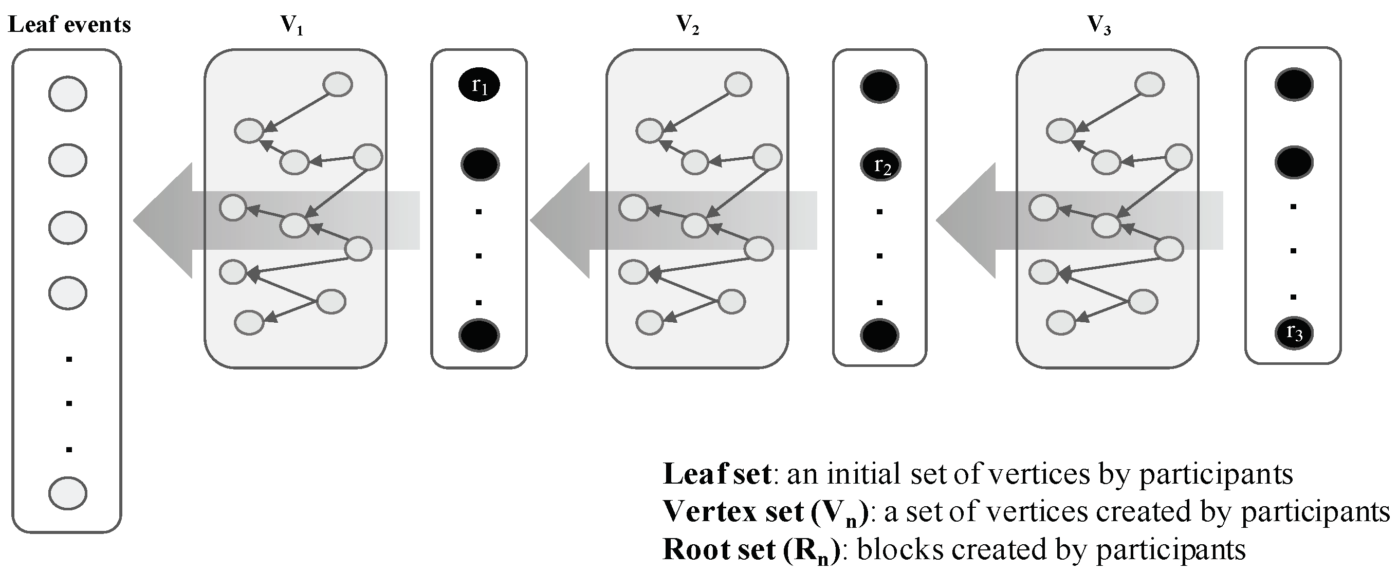
- Event block: All nodes can create event blocks at time t. The structure of an event block includes the signature, generation time, transaction history, and hash information to references. The information of the referenced event blocks can be copied by each node. The first event block of each node is referred to as a leaf event.
- Decision search protocol: Decision search protocol is the set of rules that govern the communication between nodes. When each node creates event blocks, it determines which nodes choose other nodes to broadcast to. Node selection can either be random or occur via a cost function.
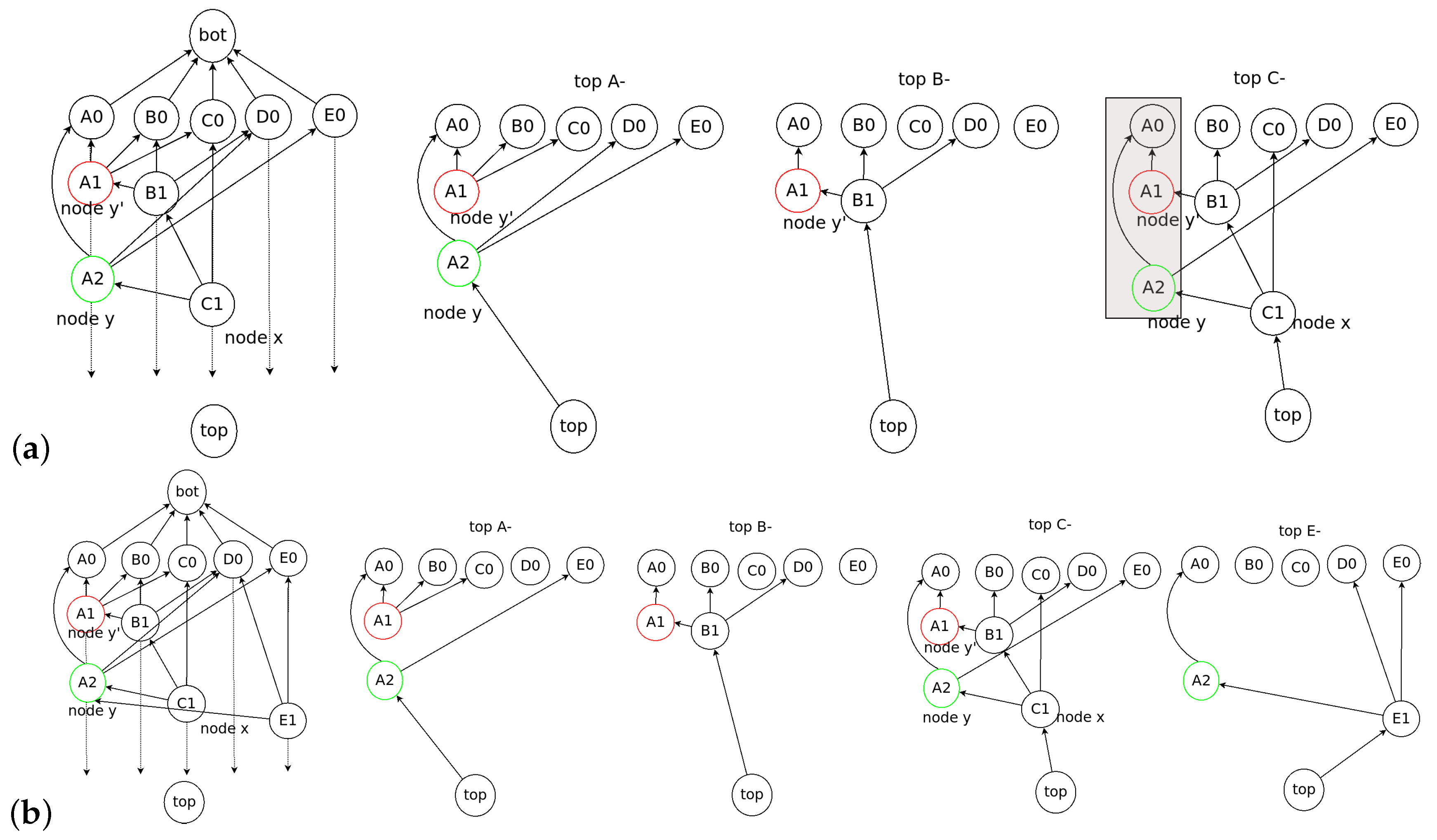
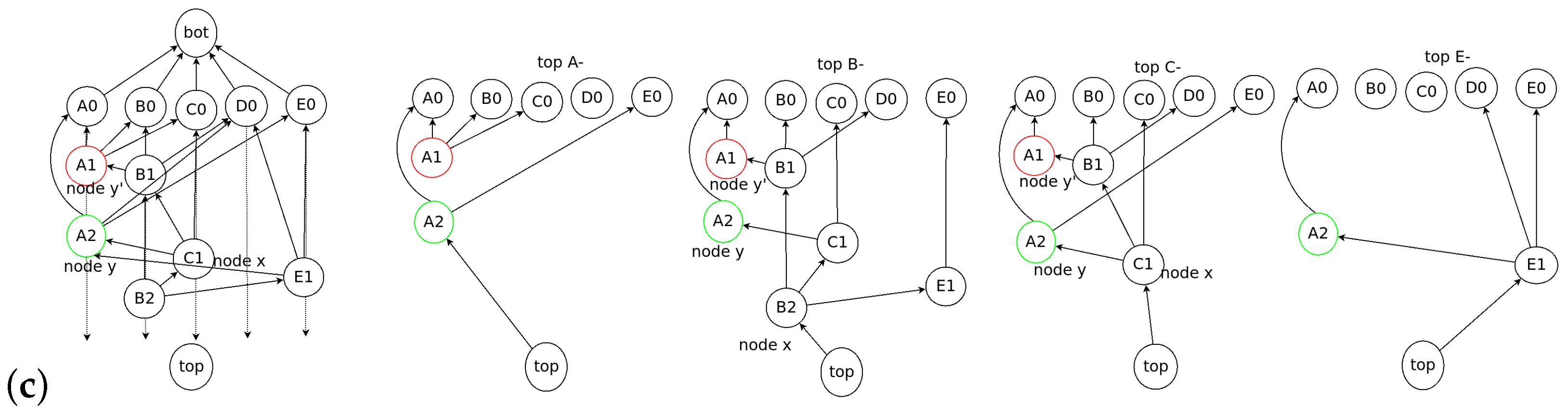
- Happened-before: Happened-before is the relationship between nodes that have event blocks. If a path exists from an event block x to y, then x is Happened-before y, which means that the node creating y knows event block x.
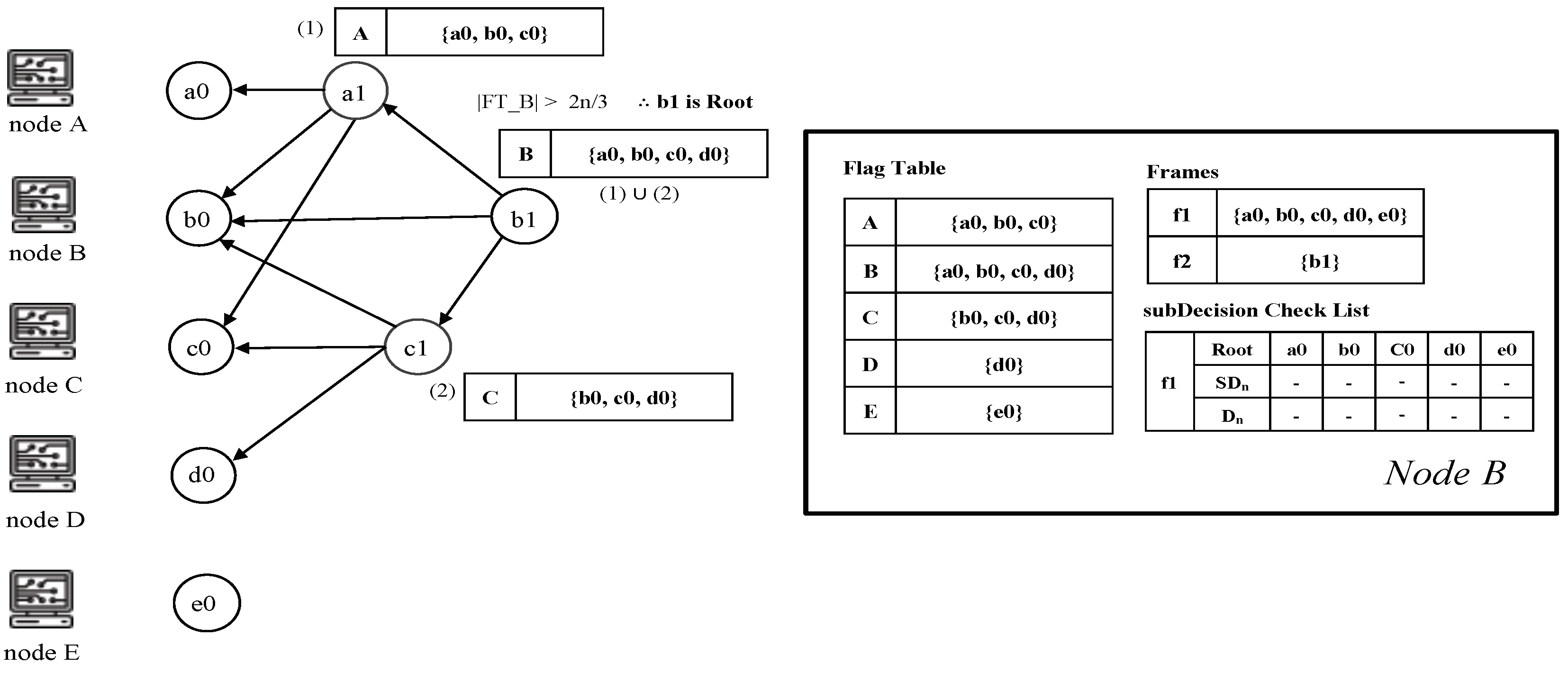
- Root: An event block is termed a Root if either (1) it is the first generated event block of a node, or (2) it can reach more than two-thirds of other Roots. Every Root can be a candidate for subDecision.
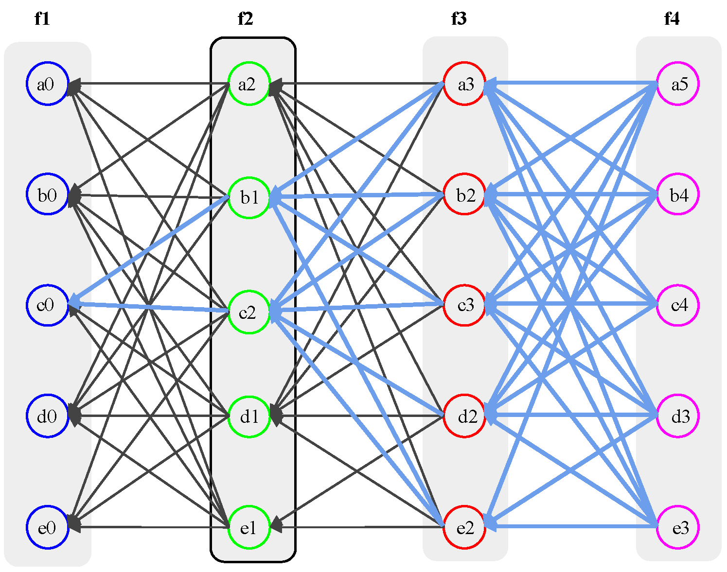
- Root set: Root set () is the set of all Roots in the frame. The cardinality of the set is n, where n is the number of all nodes.
- Frame: Frame f is a natural number that separates Root sets. The frame increases by 1 in the case of a Root in the new set (). Moreover, all event blocks between the new set and the previous Root set are included in the frame f.
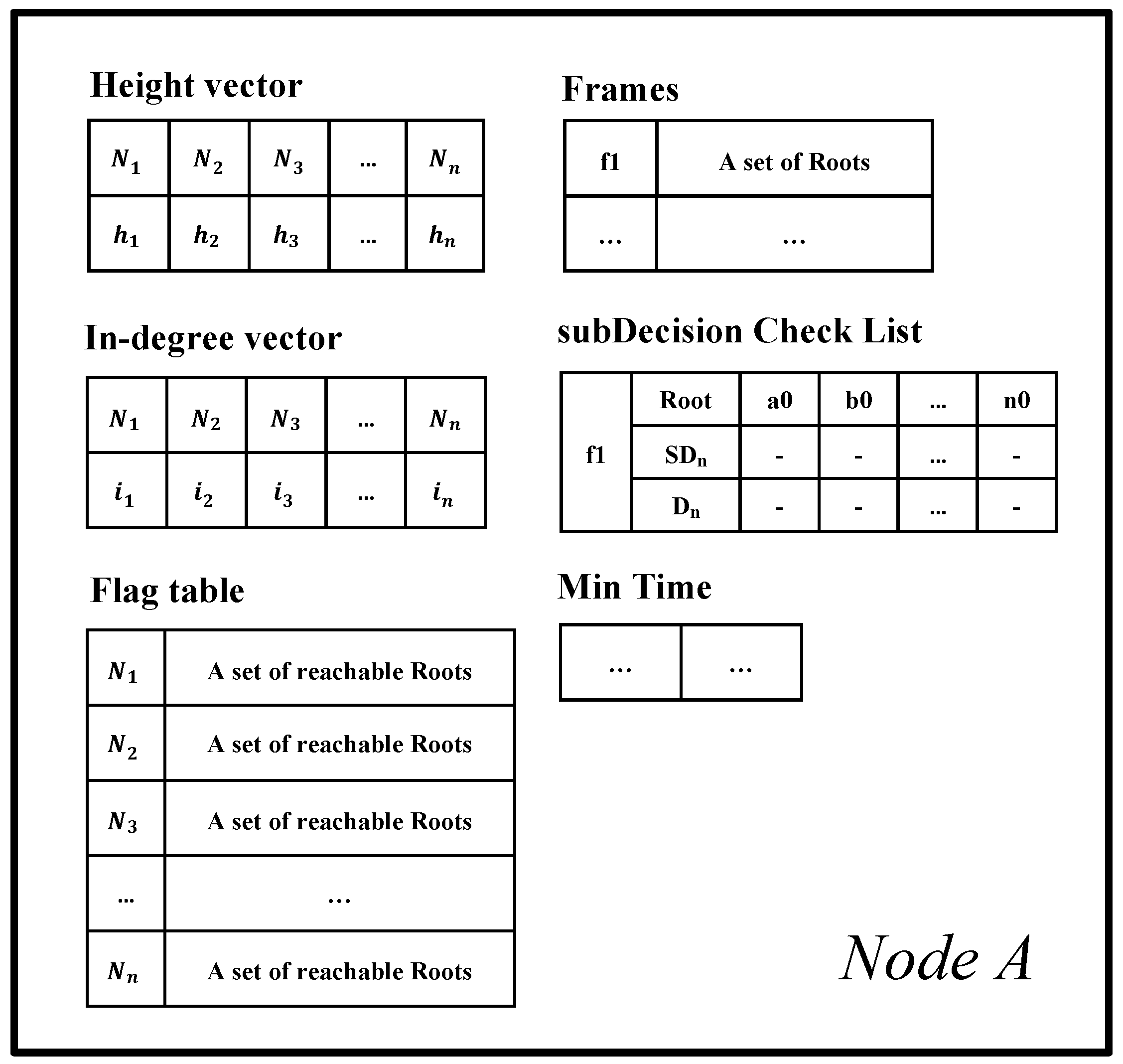
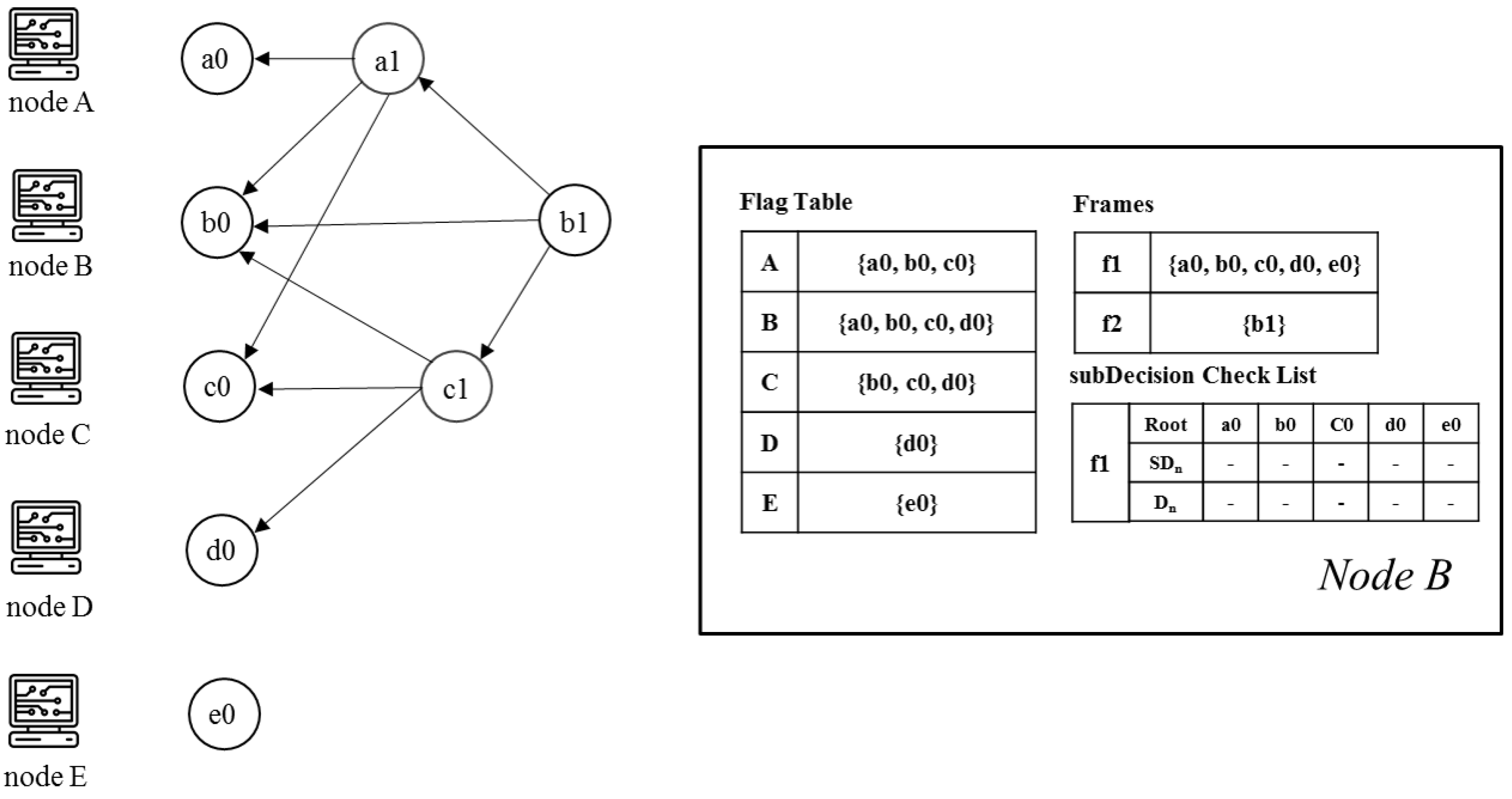
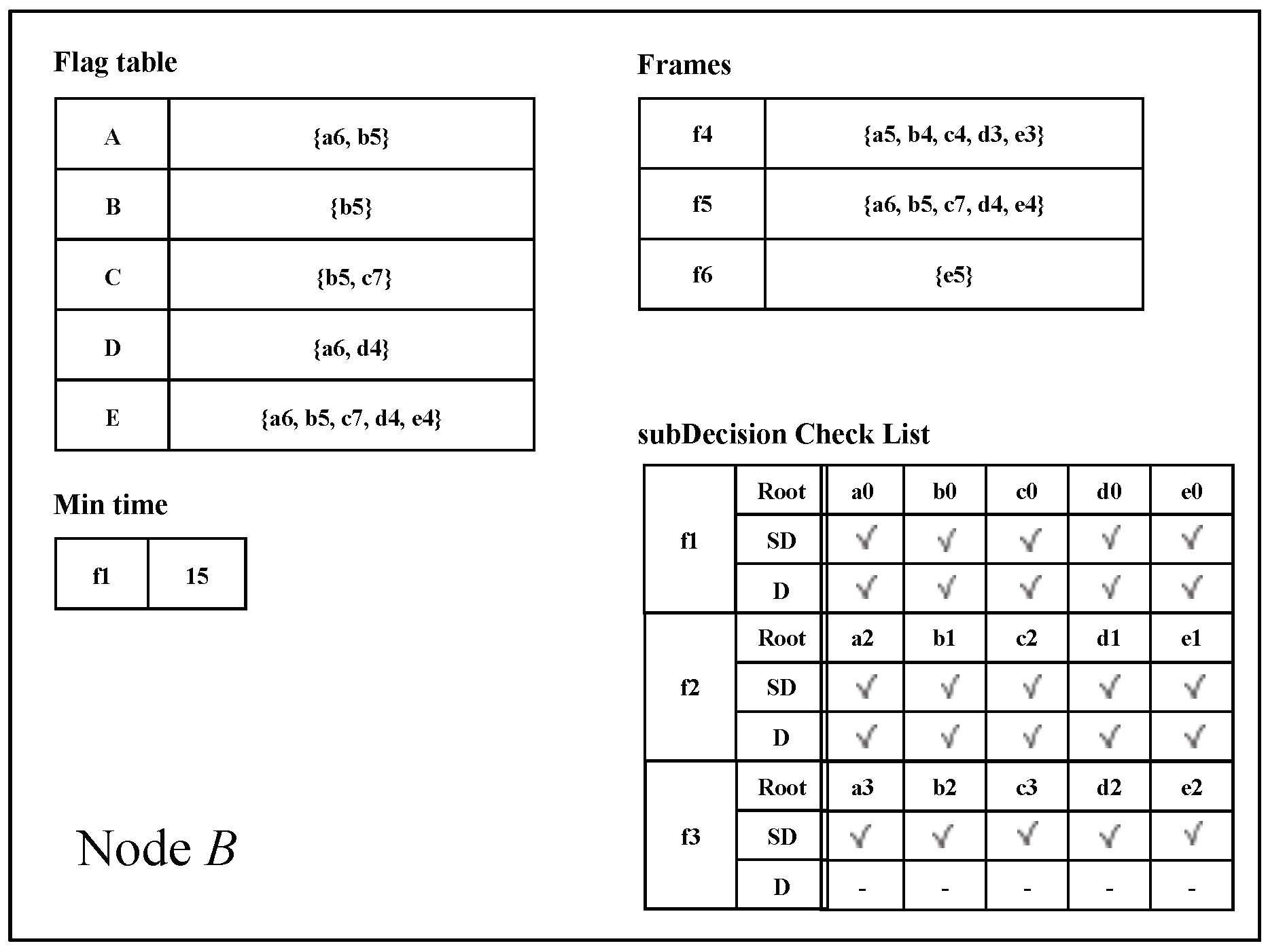
- Flag table: The Flag table stores the reachability from an event block to another Root. The sum of all reachabilities, namely all values in the flag table, indicates the number of reactions from an event block to other Roots.
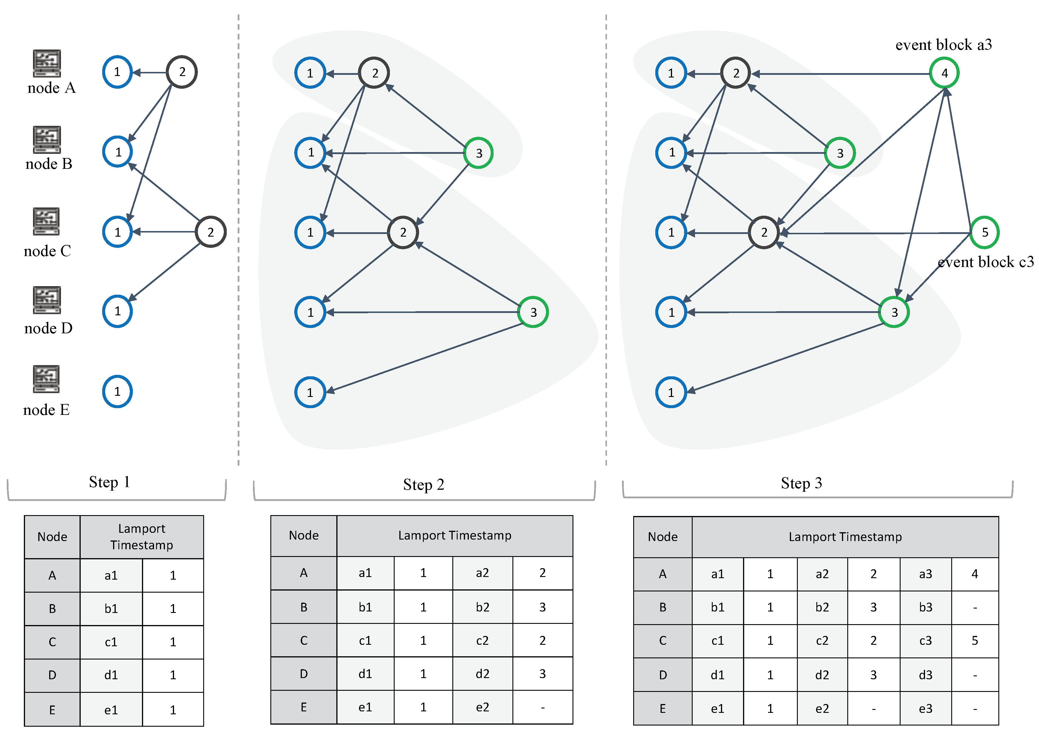
- Lamport timestamps: For topological ordering, the algorithm responsible for Lamport timestamps uses the happened-before relation to determine the partial order of the entire event block based on logical clocks.
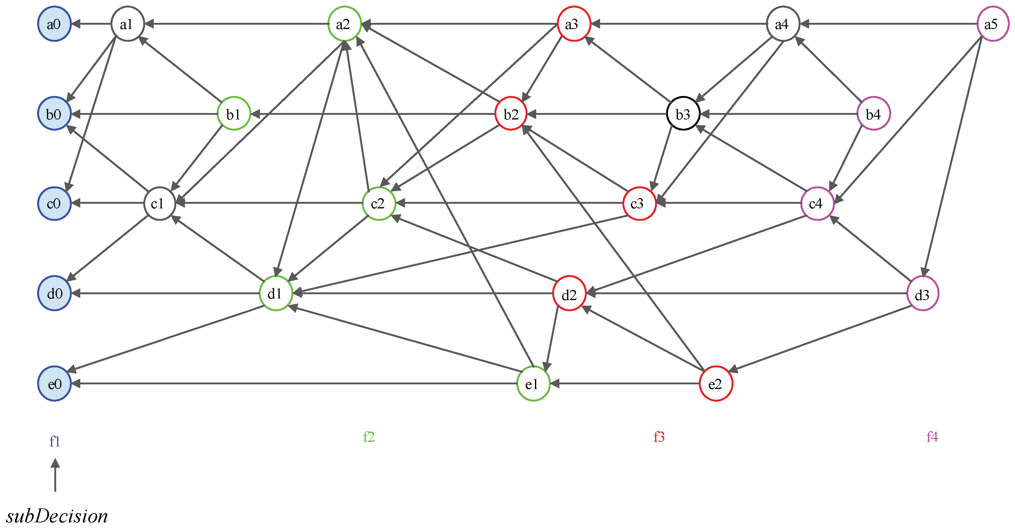
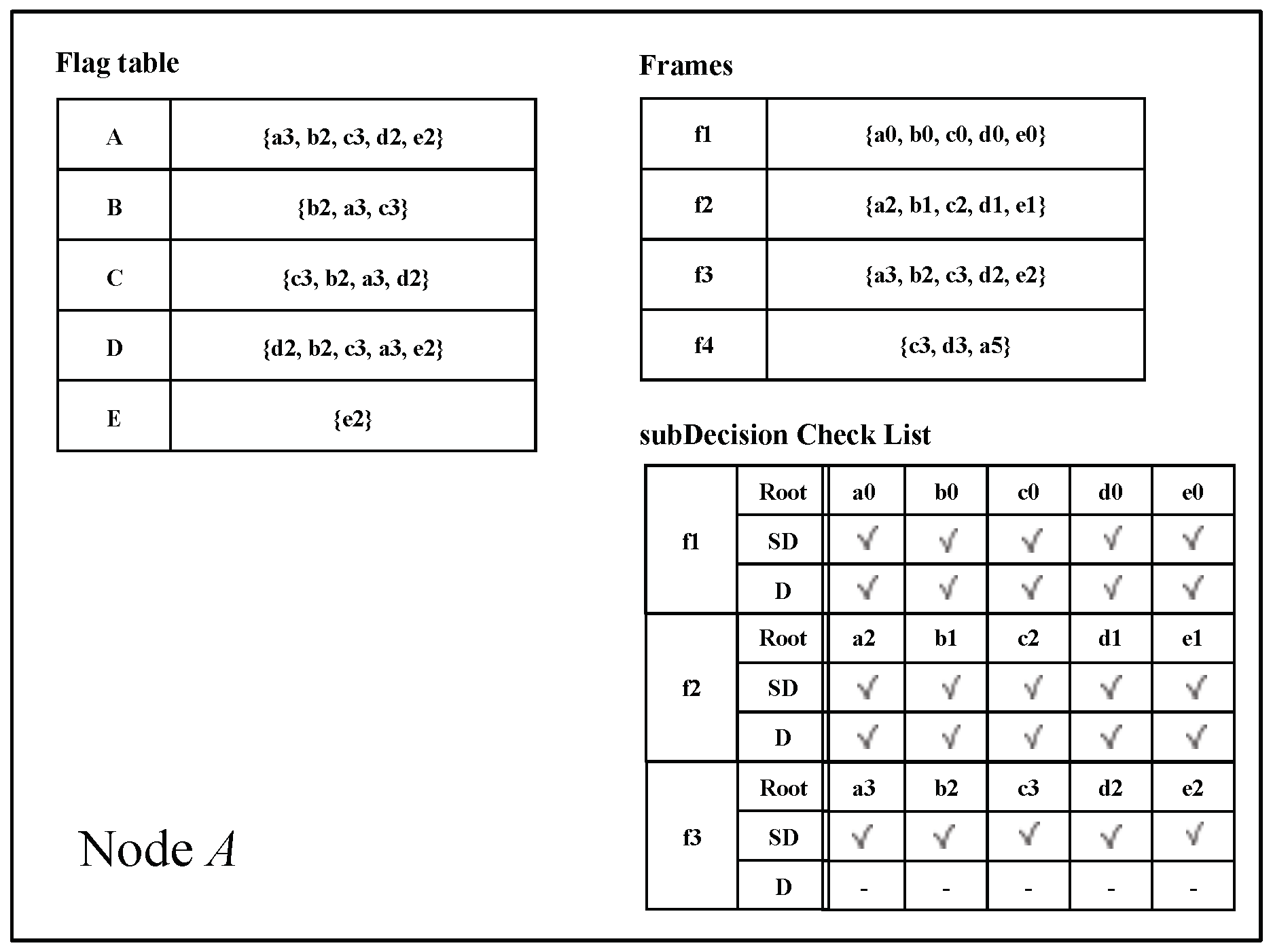
- subDecision: A subDecision is a Root that satisfies being known by more than 2n/3 nodes and more than 2n/3 nodes know the information that is known in nodes. A subDecision can be a candidate for a Decision.
- Decision: A Decision is assigned consensus time by using the Decision search algorithm and is utilized for determining the order between event blocks. Decision blocks allow time consensus ordering and responses to attacks.
- Re-selection: To solve the Byzantine agreement problem, each node reselects a consensus time for a sub-selection, based on the collected consensus time in the Root set of the previous frame. When the consensus time reaches the Byzantine agreement, a subDecision is confirmed as a Decision and is then used for time consensus ordering.
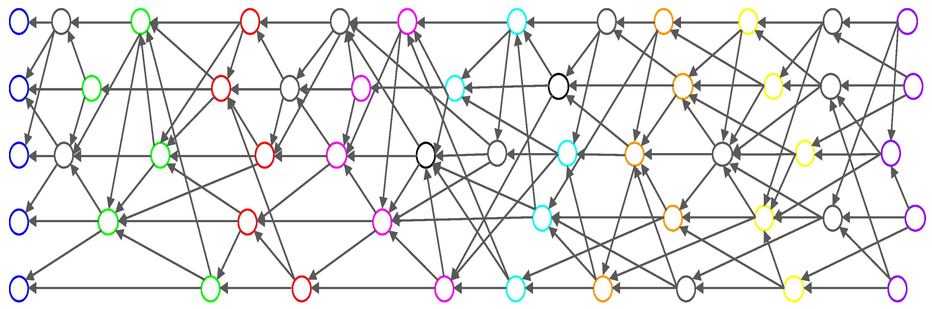
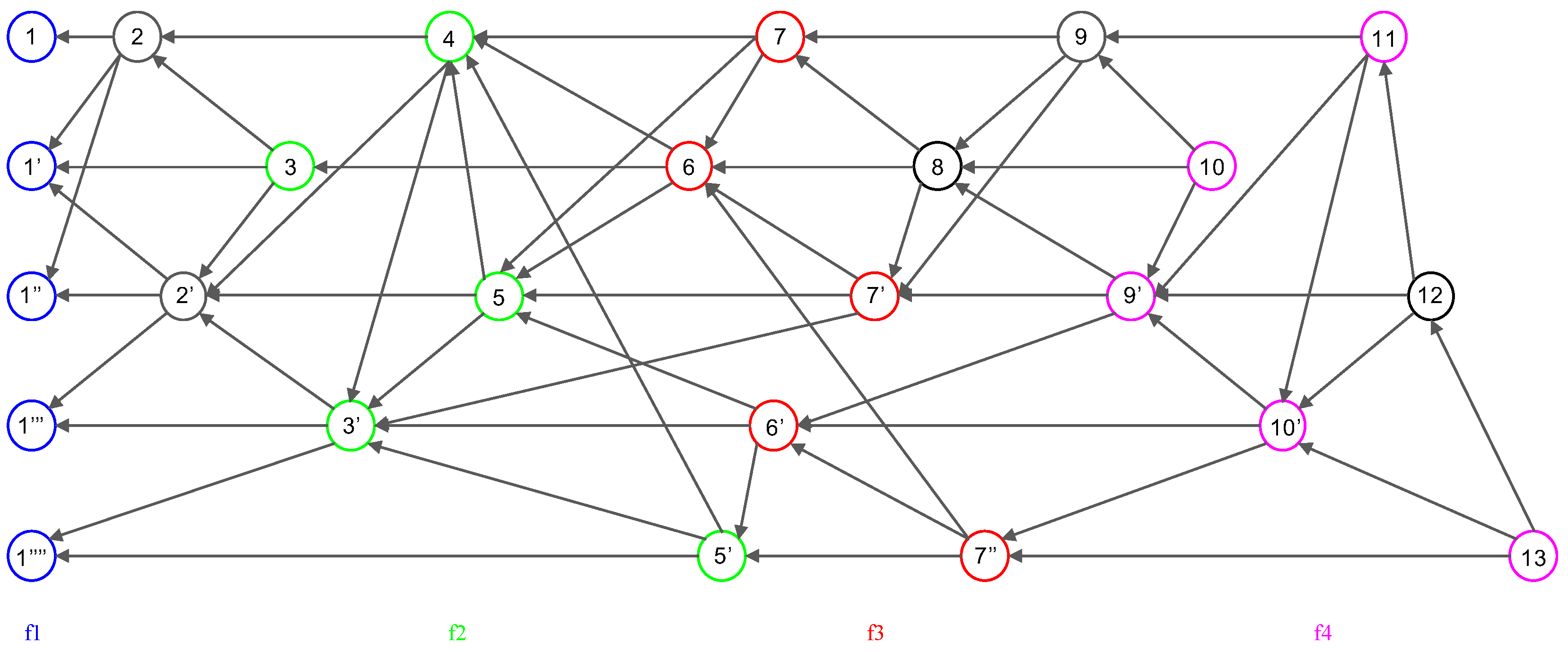
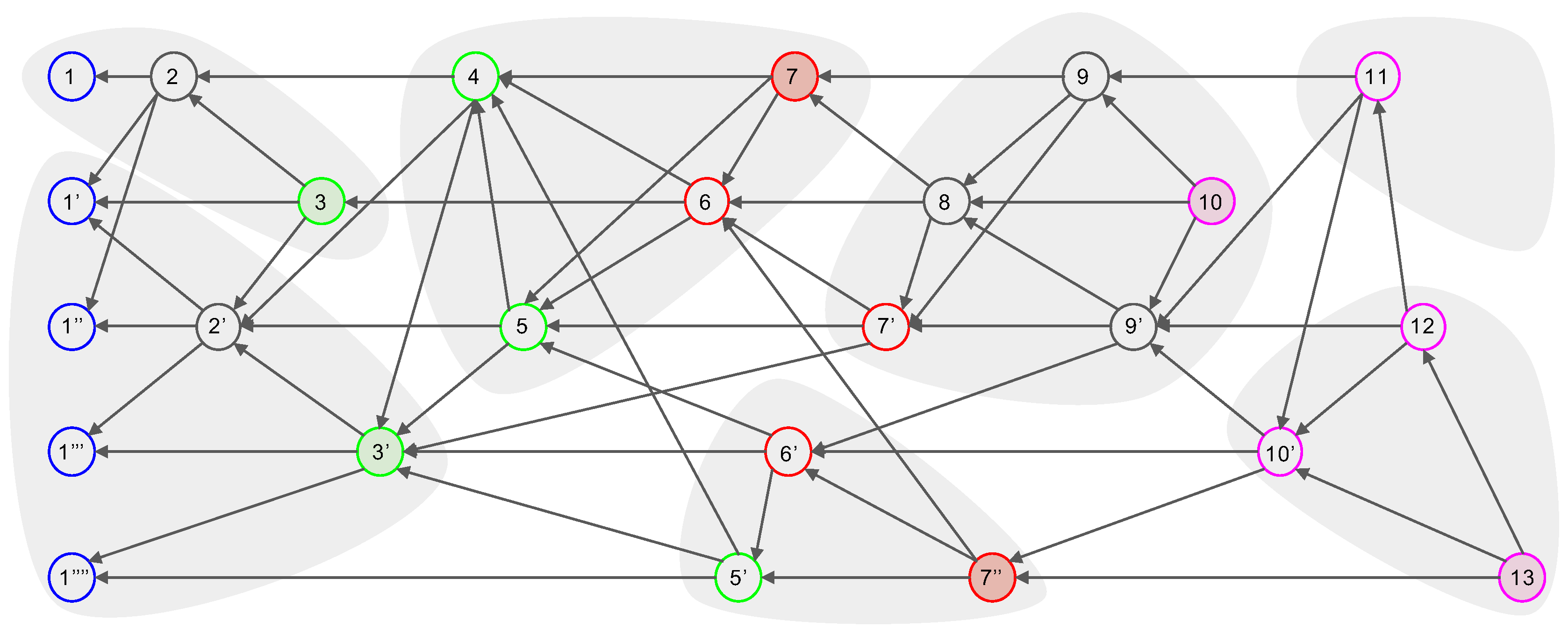
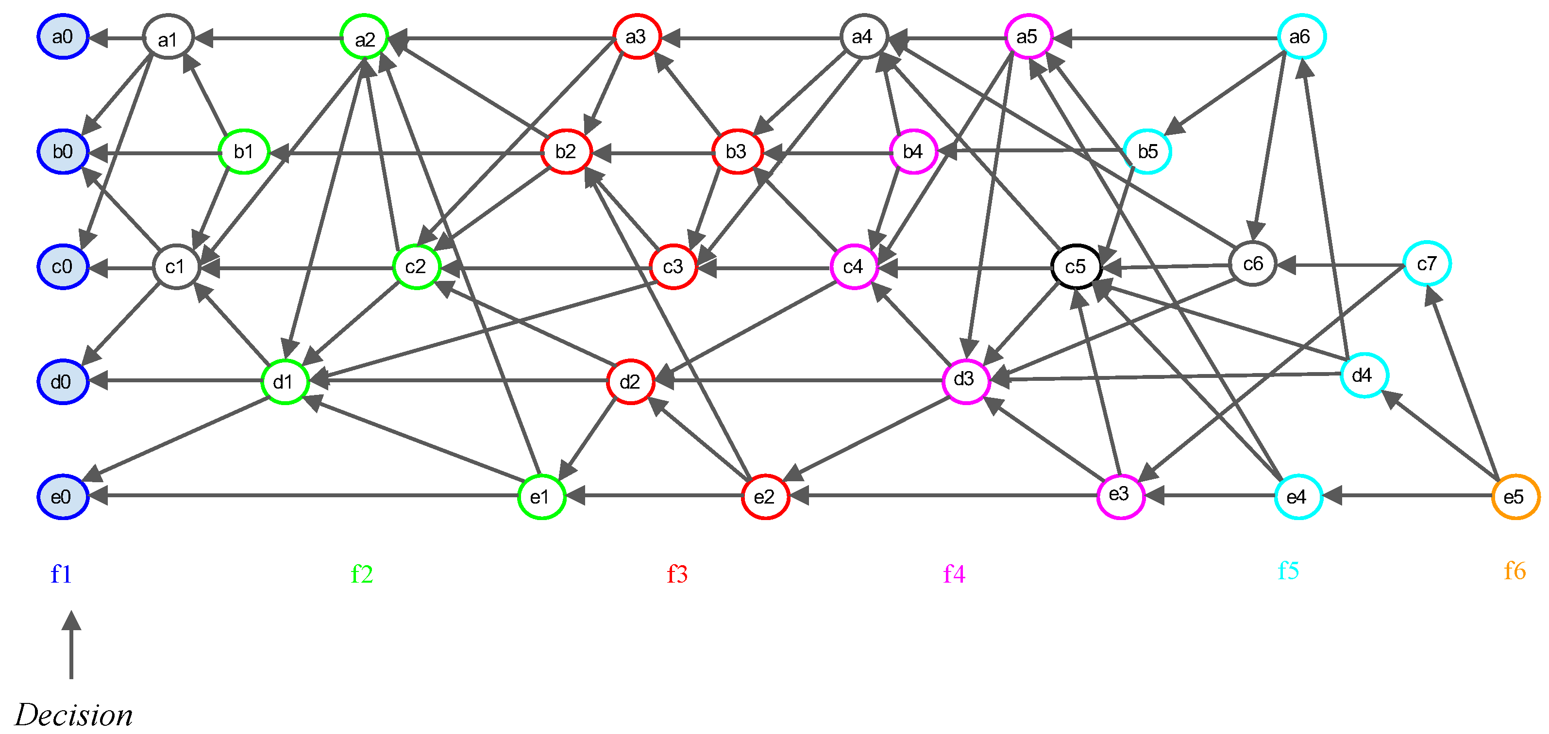
- Consensus structure: The consensus structure is the local view of the DAG held by each node, this local view is used to identify topological ordering, select subDecision, and create time consensus through Decision selection.
1.3. Decision Search Protocol
1.4. Contributions
- We propose new consensus protocols, namely Decision search protocols. We introduce the consensus structure for faster consensus.
- We define the topological ordering of nodes and event blocks in the consensus structure. Lamport timestamps are used to introduce more intuitive and reliable ordering in distributed systems. We introduce a flag table at each top event block to improve Root detection.
- We present proof of the way in which a DAG-based protocol can implement concurrent common knowledge for consistent cuts.
- The Decision search protocols allow for faster node synchronization with k-neighbor broadcasts.
- A specific Decision search protocol DecisionBFT is then introduced with specific algorithms. The benefits of the Decision search protocol DecisionBFT include (1) the Root selection algorithm via the flag table, (2) an algorithm to build the DAG, (3) an algorithm for k peer selection via a cost function; (4) faster consensus selection via k peer broadcasts;
2. Background
2.1. Related Work
2.1.1. Consensus Algorithms
2.1.2. DAG-Based Approaches
2.1.3. Lamport Timestamps
2.1.4. Concurrent Common Knowledge
2.2. Preliminaries
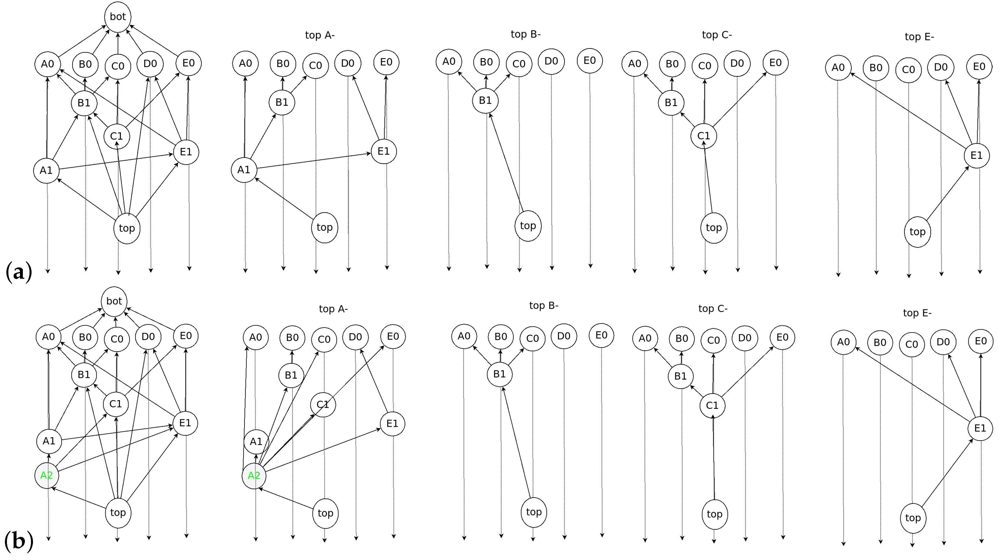
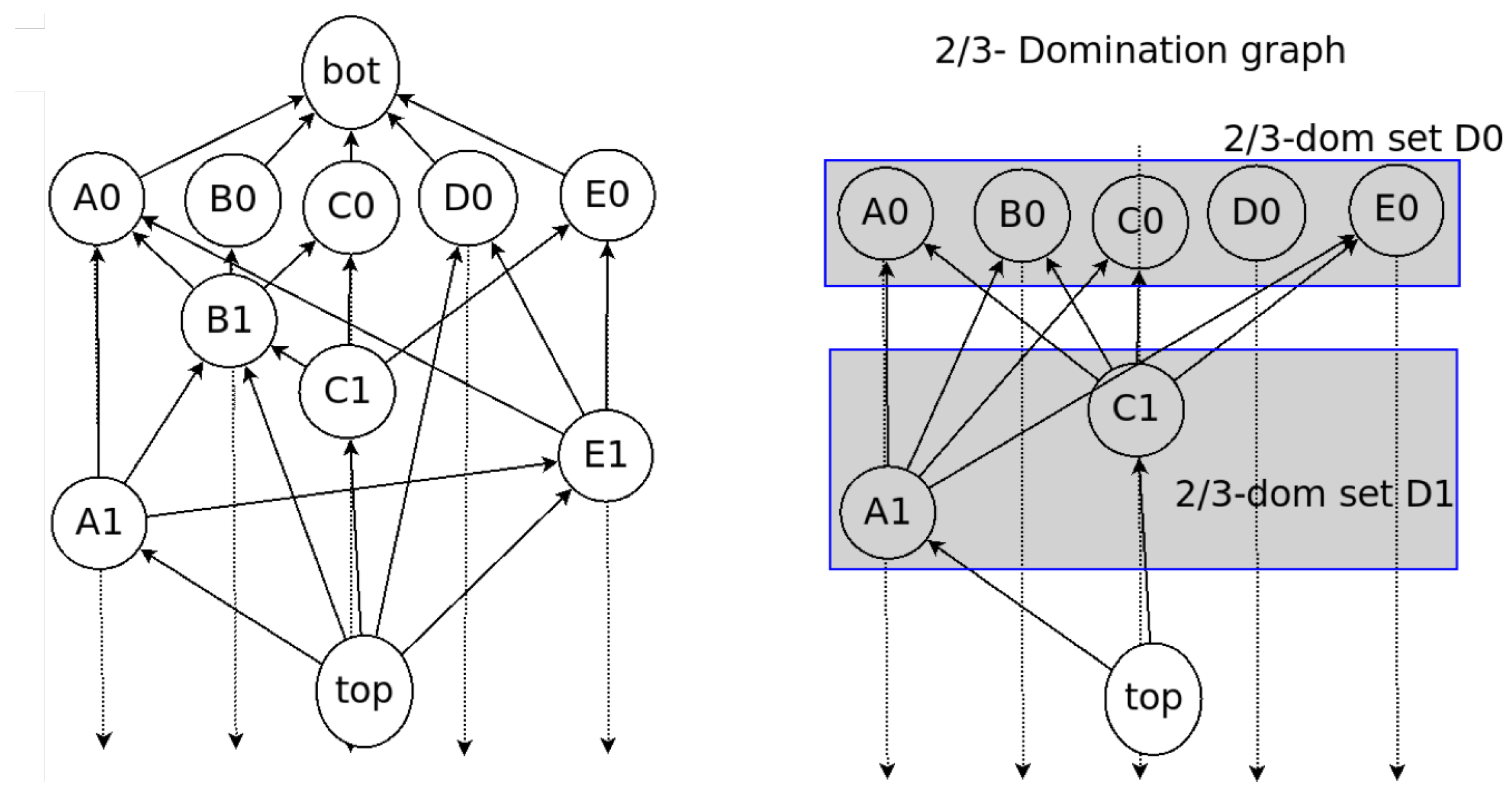
Domination Relation
2.3. Examples of Dominant Relation in Consensus Structure
3. Generic Framework of Decision Search Protocol
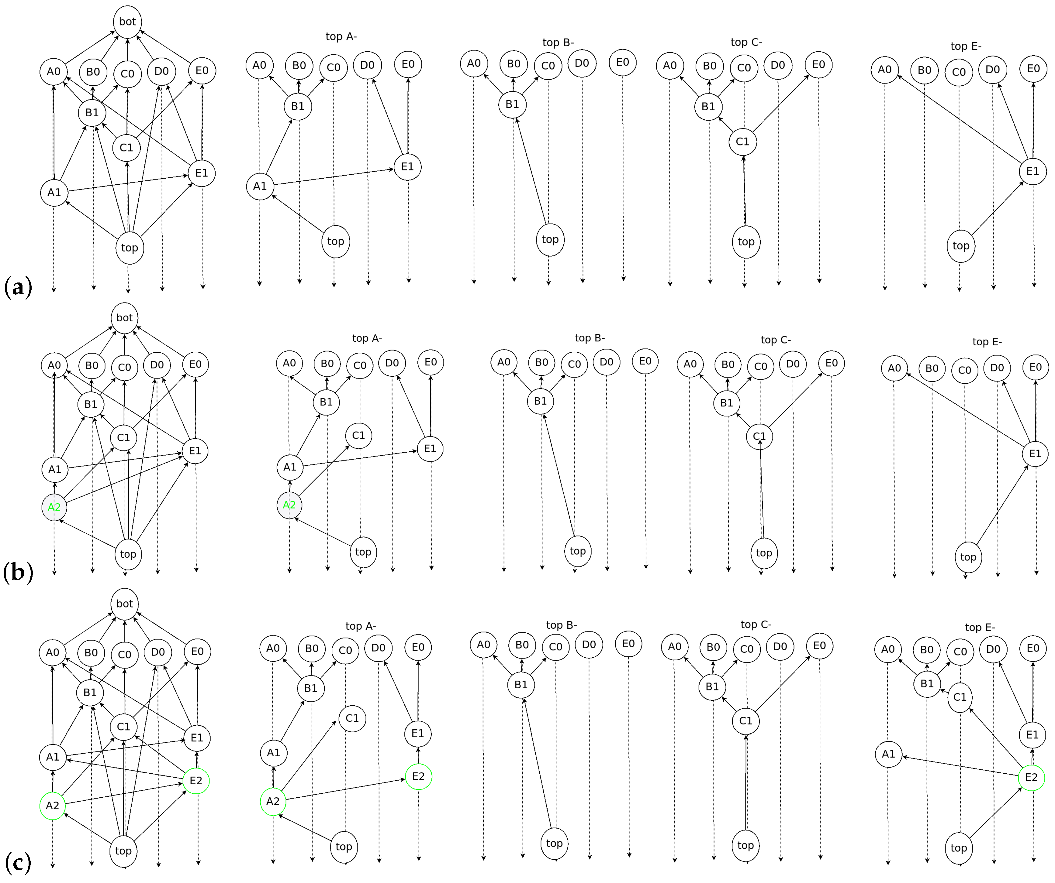
3.1. Consensus Structure
3.2. Decision Search Algorithm
| Algorithm 1 Main Procedure |
|
| Algorithm 2k-neighbor Node Selection |
|
3.3. Node Structure
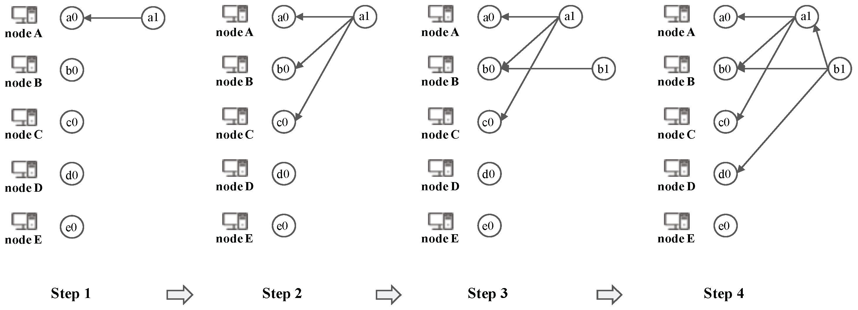
3.4. Event Block Creation
- Each of the k reference event blocks is the top event block of its own node.
- One reference should be made to a self-ref that refers to an event block of the same node.
- The other k − 1 reference refers to the other k −1 top event nodes on other nodes.
3.5. Topological Ordering of Events Using Lamport Timestamps
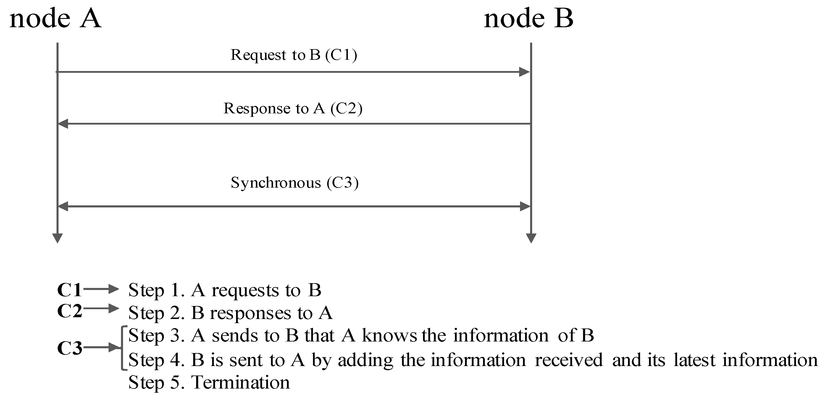
- Each node increments its count value before creating an event block.
- When sending a message that includes its count value, the receiver should consider from which sender the message is received and increment its count value.
- If the current counter is less than or equal to the received count value from another node, then the count value of the recipient is updated.
- If the current counter is greater than the count value received from another node, then the current count value is updated.
3.6. Topological Consensus Ordering
- If there is more than one Decision with different times on the same frame, the event block with smaller consensus time has higher priority.
- If there is more than one Decision with the same consensus time on the same frame, determine the order based on the own logical time from the Lamport timestamp.
- When more than one Decision has the same consensus time, if the local logical time is the same, the hash function prioritizes a smaller hash value.
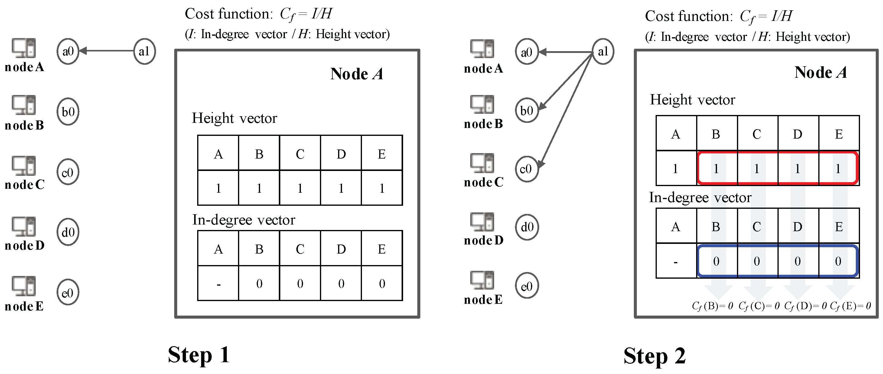
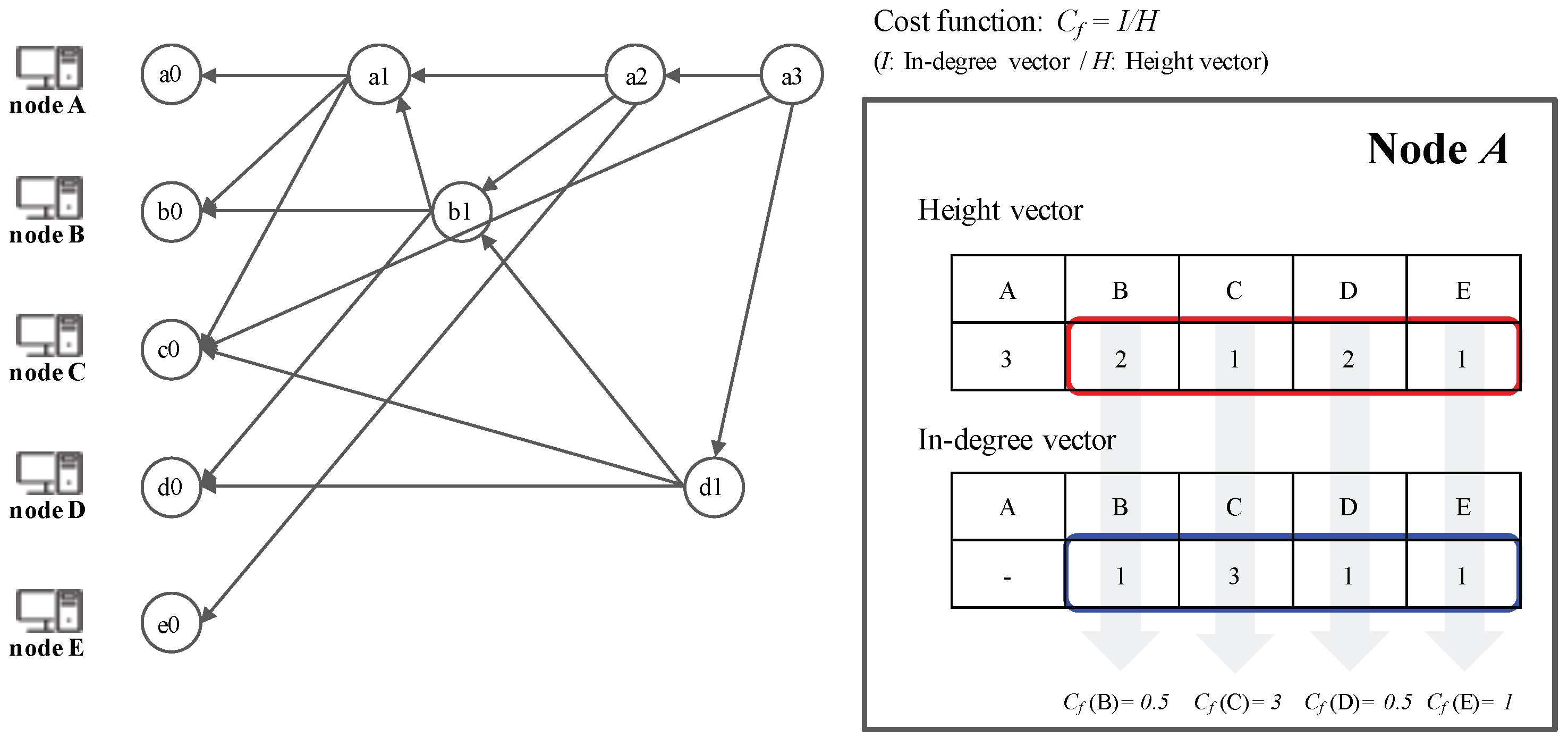
3.7. Peer Selection Algorithm
4. Proof of Decision Search Protocol
4.1. Proof of Byzantine Fault Tolerance for Decision Search Algorithm
4.2. Semantics of Decision Search Protocol
5. Decision Search Protocol DecisionBFT
5.1. Root Selection
- The first event blocks are considered as Roots.
- When a new event block is added to the consensus structure, we check whether the event block is a Root by applying an operation to each set of the flag tables connected to the new event block. If the cardinality of the Root set in the flag table for the new event block is more than 2n/3, the new event block becomes a Root.
- When a new Root appears on the consensus structure, the nodes update their frames. If one of the new event blocks becomes a Root, all nodes that share the new event block add the hash value of the event block to their frames.
- The new Root set is created if the cardinality of the previous Root set is more than 2n/3 and the new event block can reach 2n/3 Root in .
- When the new Root set is created, the event blocks from previous Root set to before belong to the frame .
5.2. subDecision Selection
| Algorithm 3 The subDecision selection |
|
5.3. Decision Selection
| Algorithm 4 Decision consensus time selection |
|
| Algorithm 5 Consensus Time Re-selection |
|
5.4. Peer Selection Algorithm via Cost Function
6. Discussions
6.1. Lamport Timestamps
6.2. Semantics of Decision Search Protocols
6.3. Dynamic Participants
6.4. Analysis of Time Complexity
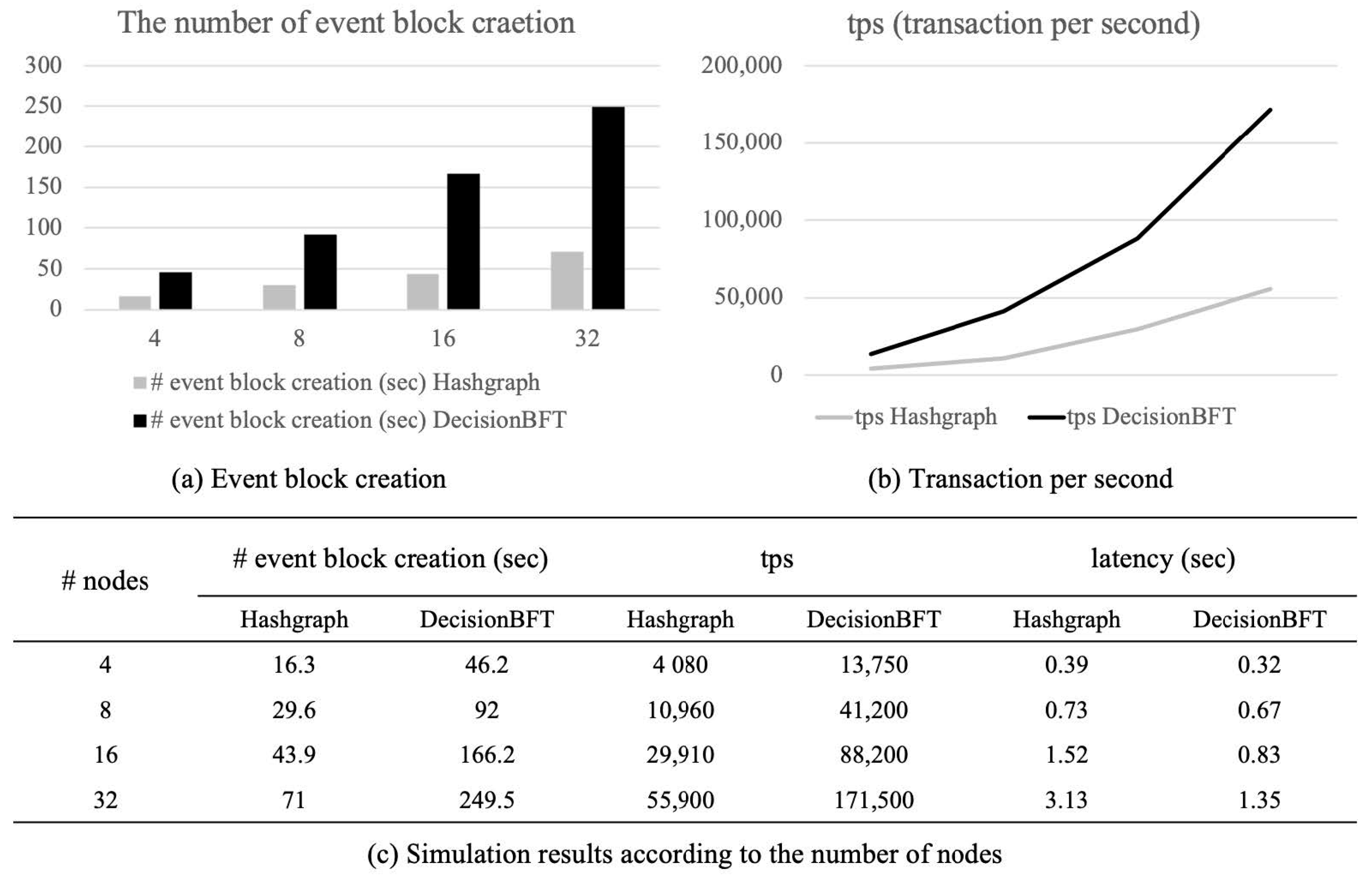
6.5. Simulation Results
7. Conclusions
Future Work
- Using the Decision search protocols, we are designing a fast node synchronization algorithm with k-neighbor broadcasts. The consensus structure and k peer selection make it possible to achieve faster gossip broadcast.
- We are interested in comparing the performance of various gossip strategies, such as random gossip, broadcast gossip, and collection tree protocol for distributed averaging in wireless sensor networks.
Author Contributions
Funding
Acknowledgments
Conflicts of Interest
References
- Swan, M. Blockchain: Blueprint for a New Economy; O’Reilly Media: Sevastopol, CA, USA, 2015. [Google Scholar]
- Chen, J.; Micali, S. Algorand. arXiv 2016, arXiv:1607.01341. [Google Scholar]
- Gilad, Y.; Hemo, R.; Micali, S.; Vlachos, G.; Zeldovich, N. Algorand: Scaling byzantine agreements for cryptocurrencies. In Proceedings of the 26th Symposium on Operating Systems Principles, Shanghai, China, 28–31 October 2017; ACM: New York, NY, USA, 2017; pp. 51–68. [Google Scholar]
- Sompolinsky, Y.; Lewenberg, Y.; Zohar, A. SPECTRE: A Fast and Scalable Cryptocurrency Protocol. IACR Cryptol. ePrint Arch. 2016, 2016, 1159. [Google Scholar]
- Sompolinsky, Y.; Zohar, A. PHANTOM, GHOSTDAG: Two Scalable BlockDAG Protocols. 2020. Available online: https://eprint.iacr.org/2018/104.pdf (accessed on 19 August 2020).
- Lamport, L.; Shostak, R.; Pease, M. The Byzantine Generals Problem. ACM Trans. Program. Lang. Syst. 1982, 4, 382–401. [Google Scholar] [CrossRef]
- Aspnes, J. Randomized protocols for asynchronous consensus. Distrib. Comput. 2003, 16, 165–175. [Google Scholar] [CrossRef]
- Lamport, L. Paxos made simple. ACM Sigact News 2001, 32, 18–25. [Google Scholar]
- Fischer, M.J.; Lynch, N.A.; Paterson, M. Impossibility of Distributed Consensus with One Faulty Process. J. ACM 1985, 32, 374–382. [Google Scholar] [CrossRef]
- Nakamoto, S. Bitcoin: A Peer-to-Peer Electronic Cash System. 2008. Available online: https://bitcoin.org/bitcoin.pdf (accessed on 19 August 2020).
- Sunny King, S.N. PPCoin: Peer-to-Peer Crypto-Currency with Proof-of-Stake. 2012. Available online: https://decred.org/research/king2012.pdf (accessed on 19 August 2020).
- Lerner, S.D. DagCoin. 2015. Available online: https://bitslog.files.wordpress.com/2015/09/dagcoin-v41.pdf (accessed on 19 August 2020).
- Chevalier, P.; Kaminski, B.; Hutchison, F.; Ma, Q.; Sharma, S. Protocol for Asynchronous, Reliable, Secure and Efficient Consensus (PARSEC). arXiv 2018, arXiv:1907.11445. [Google Scholar]
- Li, C.; Li, P.; Zhou, D.; Xu, W.; Long, F.; Yao, A. Scaling Nakamoto Consensus to Thousands of Transactions per Second. arXiv 2018, arXiv:1805.03870. [Google Scholar]
- Popov, S.; Saa, O.; Finardi, P. Equilibria in the Tangle. arXiv 2019, arXiv:1712.05385. [Google Scholar]
- Churyumov, A. Byteball: A Decentralized System for Storage and Transfer of Value. 2016. Available online: https://obyte.org/Byteball.pdf (accessed on 19 August 2020).
- Baird, L. Hashgraph Consensus: Fair, Fast, Byzantine Fault Tolerance. 2016. Available online: https://www.swirlds.com/wp-content/uploads/2016/06/2016-05-31-Swirlds-Consensus-Algorithm-TR-2016-01.pdf (accessed on 19 August 2020).
- Castro, M.; Liskov, B. Practical Byzantine Fault Tolerance. In Proceedings of the Third Symposium on Operating Systems Design and Implementation (OSDI ’99), New Orleans, LA, USA, 22–25 February 1999; USENIX Association: Berkeley, CA, USA, 1999; pp. 173–186. [Google Scholar]
- Kotla, R.; Alvisi, L.; Dahlin, M.; Clement, A.; Wong, E. Zyzzyva: Speculative byzantine fault tolerance. ACM SIGOPS Oper. Syst. Rev. 2007, 41, 45–58. [Google Scholar] [CrossRef]
- Miller, A.; Xia, Y.; Croman, K.; Shi, E.; Song, D. The honey badger of BFT protocols. In Proceedings of the 2016 ACM SIGSAC Conference on Computer and Communications Security, Vienna, Austria, 24–28 October 2016; ACM: New York, NY, USA, 2016; pp. 31–42. [Google Scholar]
- Danezis, G.; Hrycyszyn, D. Blockmania: From Block DAGs to Consensus. arXiv 2018, arXiv:1809.01620. [Google Scholar]
- LeMahieu, C. Nano: A Feeless Distributed Cryptocurrency Network. 2017. Available online: https://content.nano.org/whitepaper/Nano_Whitepaper_en.pdf (accessed on 19 August 2020).
- Lamport, L. Time, clocks, and the ordering of events in a distributed system. Commun. ACM 1978, 21, 558–565. [Google Scholar]
- Panangaden, P.; Taylor, K. Concurrent common knowledge: Defining agreement for asynchronous systems. Distrib. Comput. 1992, 6, 73–93. [Google Scholar] [CrossRef][Green Version]
- Choi, S.M.; Park, J.; Nguyen, Q.; Cronje, A. Fantom: A scalable framework for asynchronous distributed systems. arXiv 2018, arXiv:1810.10360. [Google Scholar]
- Fantom-Foundation/Fantom-Documentation. 2018. Available online: https://github.com/Fantom-foundation/fantom-documentation/wiki (accessed on 19 August 2020).


| Approach | Description | Limitation |
|---|---|---|
| IOTA [15] | The Markov chain Monte Carlo (MCMC) tip selection algorithm and DAG-based techniques | Time consuming to detect conflicts |
| Byteball [16] | Consensus ordering is composed by selecting a single main chain, which is determined as a Root consisting of the most Roots. | Time consuming to reach consensus |
| RaiBlocks [22] | A process of obtaining consensus through the balance weighted vote on conflicting transactions. | Time consuming to reach consensus |
| Hashgraph [17] | Each node is connected by its own ancestor and randomly communicates known events through a gossip protocol. | Each node maintains large information |
| Conflux [14] | DAG-based Nakamoto consensus protocol. | Time consuming to reach consensus |
| Parsec [13] | An consensus algorithm that guarantees Byzantine faults tolerance in a random synchronous network. | It allows up to one-third Byzantine (arbitrary) failures. |
| Phantom [5] | A protocol based on PoW for a permission-less ledger with a DAG concept. | Time consuming to reach consensus |
| Specter [4] | A protocol based on PoW and DAG to generalize blockchain structures. | Time consuming to reach consensus |
| Blockmania [21] | A mechanism to achieve consensus with several advantages over the more traditional pBFT protocol and its variants. | Only provides communication efficiency, not consensus protocol. |
| Symbol | Name | Definition | Example |
|---|---|---|---|
| ref | reference hash of an event block points to another event block | ||
| ⊤ | pseudo-top | parent of all top event blocks | ⊤ |
| ⊥ | pseudo-bottom | child of all leaf event blocks | ⊥ |
| ↦ | Happened-Immediate-Before | if is a (self-) ref of | |
| → | Happened-Before | if is a (self-) ancestor of | |
| ‖ | concurrent | Two event blocks are said to be concurrent if neither of them happened before the other | |
| ⋔ | fork | If two event blocks have the same creator |
© 2020 by the authors. Licensee MDPI, Basel, Switzerland. This article is an open access article distributed under the terms and conditions of the Creative Commons Attribution (CC BY) license (http://creativecommons.org/licenses/by/4.0/).
Share and Cite
Choi, S.-M.; Park, J.; Jang, K.; Park, C. Rapid Consensus Structure: Continuous Common Knowledge in Asynchronous Distributed Systems. Mathematics 2020, 8, 1673. https://doi.org/10.3390/math8101673
Choi S-M, Park J, Jang K, Park C. Rapid Consensus Structure: Continuous Common Knowledge in Asynchronous Distributed Systems. Mathematics. 2020; 8(10):1673. https://doi.org/10.3390/math8101673
Chicago/Turabian StyleChoi, Sang-Min, Jiho Park, Kiyoung Jang, and Chihyun Park. 2020. "Rapid Consensus Structure: Continuous Common Knowledge in Asynchronous Distributed Systems" Mathematics 8, no. 10: 1673. https://doi.org/10.3390/math8101673
APA StyleChoi, S.-M., Park, J., Jang, K., & Park, C. (2020). Rapid Consensus Structure: Continuous Common Knowledge in Asynchronous Distributed Systems. Mathematics, 8(10), 1673. https://doi.org/10.3390/math8101673