Is There a Connection between Sovereign CDS Spreads and the Stock Market? Evidence for European and US Returns and Volatilities

Abstract

This study complements the current literature, providing a thorough investigation of the lead–lag connection between stock indices and sovereign credit default swap (CDS) returns for 14 European countries and the US over the period 2004–2016. We use a rolling VAR framework that enables us to analyse the connection process over time covering both crisis and non-crisis periods. In addition, we analyse the relationship between stock market volatility and CDS returns. We find that the connection between the credit and equity markets does exist and that it is time variable and seems to be related to financial crises. We also observe that stock market returns anticipate sovereign CDS returns, and sovereign CDSs anticipate the conditional volatility of equity returns, closing a connectedness circle between markets. Contribution percentages in terms of returns are more intense in the US than in Europe and the opposite result is found with respect to volatilities. Within Europe, a greater impact in Eurozone countries compared to non-Eurozone countries is observed. Finally, an additional analysis is also carried out for the financial sector, obtaining results largely consistent with those found using sovereign data.

1. Introduction

After the Lehman Brothers default in September 2008, international financial markets experienced devastating distortions, highlighting the importance of the study of risk management, especially credit risk, for both academics and professionals. This interest has been revived in recent years in the context of the European debt crisis, where credit spreads rose to unprecedented levels, to a greater extent in the Eurozone countries. As a result, there is an undeniable interest in understanding credit risk and its relationship to other financial markets. The present paper follows this line of research, focusing attention on the connectedness between the credit default swap (CDS) market and the stock market. Specifically, we look into the risk transmission process through the price discovery mechanism. The importance of this lead–lag relationship has increased in recent years as credit derivatives have been trading in all financial markets, with CDSs being the most commonly used instrument for the transfer of credit risk.

The main lines of research that analyse the relation between the stock and the credit market have used equity prices and bond spreads [1,2]; however, some literature has shown that CDS spreads anticipate first and have more impact on stock returns than bond credit spreads [3,4,5]. Nowadays, the results regarding the lead–lag relationship between these markets are not conclusive. Initial papers for the US corporate market mostly conclude that stock returns lead CDS returns [6,7,8]; however, other studies focus on the 2008 financial crisis, either for the US or for Europe, and provide mixed results. Some authors find a significant causality from equity to CDS returns, which increases during the crisis [9,10], others show the opposite unidirectional relationship from CDSs to equity returns [11,12], or even a significant feedback in the case of high-yield CDSs [13]. More recent papers that include the sovereign debt crisis period also obtain contradictory results. The authors of [14] conclude that equity returns dominate the price discovery process, while [15] find that sovereign CDSs lead the information transmission during the sovereign debt crisis. Given this background, it is imperative to contribute to this line of research.

Furthermore, within this same family of papers, we observe that the studies that analyse the transmission process in terms of volatilities generally point to the leadership of CDSs over stocks. However, the existing literature on this topic is quite limited and also mainly focused on the US corporate market [11,12,14,16]. Therefore, we think that the analysis of the interaction between these two markets in terms of volatilities complements the analysis on returns, since it would provide information and close the circle of relationships between CDS returns, stock returns and stock return volatilities. Considering that the volatility of the financial markets experienced spectacular increases during the crisis periods, we want to explore this topic.

Accordingly, the aim of this paper is to analyse information transmission in the US and Europe between the stock market and the CDS sovereign market in terms of returns and volatilities, using a sample period that runs from 2004 to 2016. Following the methods used in recent literature, we use a vector autoregressive (VAR) model to study the lead–lag relationships, and more specifically the Granger causality, as a channel of potential transmission between both markets. As we want to capture the dynamic relationship in our data, we carry out the study in terms of a rolling window analysis.

We can break down the main objective of this paper into the following questions. Do stock returns anticipate CDS returns, or is it the other way round? Is this relationship in the same direction for stock market conditional volatility and CDS returns? Are the lead–lag relationships different between Eurozone and non-Eurozone countries and/or different among Eurozone countries? Do these transmissions vary over time? To what extent have the different crises influenced the connection between the two markets?

Our findings clearly show, for both the US and Europe, that while equity returns lead sovereign CDS returns, it is sovereign CDS returns that anticipate the market information rather than the stock market volatilities. This connectedness varies over time and is closely related to the financial crises. Causality only occurs during bad economic times, both in Europe and the US, although in the case of some Eurozone countries it is also found in the post-crisis period. Furthermore, the information transfer is more intense in the US than in Europe for the returns model, while the opposite result for the volatility model is found. In both analyses, the number of causalities is higher for Eurozone than non-Eurozone countries. There are also some differences between Euro-core and Euro-peripheral countries, depending on the sub-period considered. For instance, during the sovereign debt crisis, we find significant causal relationships between sovereign CDS returns and stock returns in those Euro-peripheral countries most affected by this crisis.

As an additional analysis, we also carry out the study using financial data. In the wake of the latest financial crises, concerns about the solvency or credit risk of many of the largest European and US banks have increased and the vulnerability of the financial system is still an important issue. We aim to check if a lead–lag relationship exists between financial stocks and CDSs and also whether or not this connection is similar to our previous sovereign results. We wonder to what extent the particular characteristics of the different crises have changed the transmission dynamics or even the practices of financial institutions. In general, the results obtained for the financial sector are in line with those previously obtained for the sovereign sector. There is clear leadership from the equity market in terms of returns and the opposite relationship in volatilities.

This study may have important implications with respect to understanding the transmission of international credit risk. The historical and current levels of transmission channels represent crucial information in terms of understanding the dynamics of risk transmission and can assist the formulation of effective and coordinated policy initiatives. The analysis of time varying correlations and price discovery processes between the CDS market and the stock market are important in terms of portfolio management in order to allocate financial assets in particular portfolios. In addition, investors, traders and policymakers are interested in the CDS–stock link in order to introduce their appropriate strategies.

The remainder of the paper is organised as follows. In Section 2, the previous literature is reviewed. Section 3 describes the data, including a preliminary statistical analysis. Section 4 presents the rolling VAR methodology. Section 5 shows the empirical results between stocks and sovereign CDS returns while Section 6 provides the analysis between the conditional volatility of stock returns and CDS returns. Finally, Section 7 presents the additional analysis results for stock and CDS financial data. The paper finishes with a brief conclusion in Section 8.

2. Literature Review

An important strand of literature (see, among others, [1,2,4]) has studied the relationship between the stock and the bond market. They conclude that an inverse relationship between these markets exists and that positive stock returns are linked to negative credit spreads due to the reduction in the firm’s default risk. With the launch of the CDS market in 2000, the possible connectedness between the stock market and the CDS market has been studied for approximately the last ten years. Thus, it can be affirmed that the line of research that this paper follows is relatively new.

In terms of returns, [3] show for 68 US firms that price discovery transmission flows first into the CDS and stock markets, and then into bond spreads. In addition, The authors of [4,5] find that stock returns have more impact on CDS spreads than on bond credit spreads for 33 European and US firms and 24 international firms. These results helped to boost interest in the link between equity and CDS spreads as substitutes for bond spreads. Regarding market volatility, reference [17] conclude for US data that increases in stock volatility explain the cross-sectional variation in corporate bond yields. Nevertheless, this paper leaves open the question as to whether this result will be confirmed for CDS returns. In this regard, The authors of [18] offers preliminary results using different statistical proofs for the connection between the CDS and the stock market jointly for returns and volatilities. Using data from European sectoral iTraxx CDS indices from 2004 to 2005, the author concludes that CDS spreads are inversely correlated with stock prices and the opposite relationship is found between CDS spreads and stock market volatilities.

The literature has focused mainly on analysing the relationship in terms of returns using corporate US data. Although most studies show that equity markets lead CDSs, the results are not conclusive. The few studies that do analyse the financial sector also offer mixed results. In the volatility analysis, there seems to be a greater consensus, with CDSs being the leaders of the transmission. However, the literature in this regard is very limited. Moreover, as we will see below, it is quite difficult to draw conclusions, regardless of whether the analysis is in returns or volatilities, due to the disparity of data, methodologies and sample periods used in the different papers.

The initial studies that analysed the relationship between both markets in terms of returns considered corporate US data. The authors of [6] analyse for 58 international firms the co-movement between both markets, finding that stock returns lead the CDS market during 2000–2002. Following the same line, The authors of [7] investigate simultaneously the discovery process in the CDS, bond and stock markets for 17 US and European non-financial firms during 2001–2003. Using stock market implied credit spreads instead of stock returns, they show that stocks lead CDSs and bonds more frequently than the opposite. More recently, the empirical evidence shown by [8] is in line with previous results for a sample of 783 US firms during 2001–2007. CDS returns do not react to equity returns, but equity returns do respond to credit returns; however, some papers document the opposite effect. In this regard, reference [19] provide empirical evidence that there is an information flow from corporate CDSs to equity for 79 US entities from 2001 to 2004. This transmission is related to bad news from a specific firm, being more significant for entities with a greater number of bank relationships and a higher credit risk.

As a result of the credit crunch of July 2007, there has been a revival in the literature focused on US data. The authors of [20], with a sample of 193 US firms during 2004–2008, find a clear advantage for stock over CDS returns in incorporating new information, mainly due to the positive information in the stock market. According to reference [13], for US stock and CDX indices from 2004 to 2007, they found that the stock market appears to lead both the investment-grade and the high-yield CDS markets. However, high-yield CDSs have more impact on the stock market than investment-grade CDSs. Moreover, they also conclude that volatilities of both CDS indices seem to lead stock market volatility. In the same line, although using exclusively large financial institutions, The authors of [11] analyse the interactions between the CDX and iTraxx indices and 15 US and European bank stock prices for the 2005–2008 period. They affirm that both indices are negatively correlated to the equity returns for all the financial institutions. In addition, they conclude that CDS volatilities had a large impact on stock market volatilities. In the same spirit of co-movements, [21], looking at 13 large US financial institutions during 2007–2008, conclude that the stock and CDS markets become more integrated in times of stress and that the stock market leads the credit market. It should be noted that the last two papers are the only ones that focus exclusively on the financial sector, but offer contradictory results.

With a broader sample period that spans 2004 to 2012, The authors of [10] classify S&P stocks into 10 different sectors. They find that the stock and the CDS markets contribute to price discovery in six out of ten sectors; however, the equity returns dominate the price discovery process. Moreover, the contribution is higher during the 2007 financial crisis compared to the non-crisis period. Following the objective in the previous study, The authors of [12] studies the connection between US markets in a dynamic contagion analysis for sectoral stock returns and volatilities and CDS returns during 2004–2012. However, the main results disagree with [10]. The shocks in CDS returns explain most of the forecast error variance of the sectoral stock returns and sectoral equity volatility, with this effect being different across sectors. Moreover, this CDS leadership is more important in terms of returns rather than volatilities, and increased during the post-crisis period. More recently, [22], looking at eleven US sectors during the period 2007–2014, reveal that the stock market leads the CDS market for all industries, and a bidirectional transmission for the banking, healthcare and materials sectors is found. Following the study of this nexus at the US sectorial level, The authors of [16] analyse the extreme dependence and nonparametric asymmetric causalities, so that causality is associated with certain quantiles. They use data from 2007 to 2015 and find evidence of unidirectional causality from equity to CDSs, but also the opposite, from CDSs to equity, depending on the sector and the quantile. For example, in the case of the financial sector, equity (CDS) leadership occurs in the average and upper quantiles (in the extreme lower quantile). On the other hand, their volatility analysis reveals bidirectional causality for all the sectors. In a recent paper, [14], for corporate US data from 2007 to 2020, the authors obtain a unidirectional causality from stock to CDS returns. Additionally, they include the VIX index as an approximation of the volatility of stocks and conclude that the VIX leads the CDS indices.

There is also no consensus among the few papers that use European data. The authors of [9] examine the relationship between iTraxx CDS with European and US stock indices during the period 2007–2009. Their results suggest that stock market returns lead the transmission with an increasing effect during the subprime crisis. In addition, financial equity and CDS indices cover most of the relationships. Using stock market implied credit spreads instead of stock returns, the authors of [23] analyse the potential factors that explain the relationship between both markets. Using data from 92 European firms during 2002–2008, they conclude, in line with reference [9], that the stock market tends to lead in periods of financial crisis. However, they also observe a higher contribution from CDSs during tranquil periods. In the wake of the Eurozone sovereign debt crisis, the authors of [15] revive the importance of studying this link. Using data from eight European countries during 2007–2010, they find that equity returns lead sovereign CDS spread changes for the full sample period and during the global crisis; but in contrast, in the sovereign crisis, the CDS market influenced the stock market, with the effect being most significant in countries with high-risk spreads. They include implied market volatility in the model, but no evidence of a connection exists with the CDS returns.

This paper complements the earlier literature, providing an exhaustive investigation of the interaction between stock and credit markets. Previous studies have essentially focused on the US corporate sector while paying little attention to the sovereign relationship. As far as we know, the only paper that uses sovereign data is reference [15], but their sample period ends in 2010, covering only three years. We improve on their study in several respects. We include the US and more European countries, and also compare the directionality of the result within Europe and inside the Eurozone, using a relatively long time period (2004–2016), which allows us to analyse the transmission dynamics between both markets in distinct crisis periods of a different nature. In this regard, as a novel contribution, we provide evidence of the time variation of the lead–lag relationship by a rolling framework, which enables us to analyse the evolution over time as well as the quantitative contribution of causalities for both crisis and non-crisis periods.

Moreover, we add additional insight with respect not only to the interaction in terms of returns, but also between stock volatility and CDS returns, hardly studied to date. As an additional proof, noting that very few papers use financial data for both the US and especially for Europe, we also carry out the analysis with financial data. We aim to contribute to the understanding of how financial institutions are interrelated and exposed to other financial markets, which is essential for the assessment of the risks to financial stability derived from these institutions. Thus, in short, the main objective of this paper is to contribute to a deepened understanding with a detailed study of the subject.

3. Data and Preliminary Analysis

We use two major datasets. With respect to the CDS market, we consider the 5-year CDS contracts since these instruments are known to be the most liquid and constitute the majority of the entire CDS market. The CDS spread indicates the 5-year CDS premium mid expressed in basis points. We have daily data of sovereign CDSs from 6 January 2004 to 12 April 2016, collected from the Thomson Datastream database, for the US and 14 developed European countries: Austria, Belgium, Denmark, France, Germany, Greece, Ireland, Italy, the Netherlands, Norway, Portugal, Spain, Sweden and the UK.

Our second dataset contains daily data of stock indices for each country, also obtained from Datastream for the same period as the CDS data, which results in 95,767 unbalanced panel observations. Specifically, we collect data for the following stock indices: ATX (Austria), BEL20 (Belgium), OMX 20 (Denmark), CAC40 (France), DAX30 (Germany), ATHEX COMPOSITE (Greece), ISEQ (Ireland), FTSE MIB INDEX (Italy), AEX (Netherlands), OSLO EXCHANGE ALL SHARE (Norway), PSI20 (Portugal), IBEX35 (Spain), OMXS30 (Sweden), FTSE 100 (UK) and S&P 500 (US). The sample period covers a relatively long time period (2004–2016), which enable us to analyse the dynamic relationship between the stock and credit markets.

Table 1. Main descriptive statistics of daily stock indices and sovereign credit default swap (CDS) spreads.

	Sovereign CDS					Stock Indices
Zone/Country	Obs.	Min.	Max.	Mean	Std. Deviation	Obs.	Min.	Max	Mean	Std. Deviation
Eurozone
Euro-core
Austria	3201	0.50	273.00	46.15	52.86	3201	1411.95	4981.87	2772.64	844.92
Belgium	3201	1.00	398.78	63.84	75.60	3201	1527.27	4756.82	3009.51	715.07
France	2781	0.50	245.27	53.86	52.60	3201	2519.29	6168.15	4193.40	761.66
Germany	3199	0.60	118.38	25.24	25.47	3201	3646.99	12,374.73	6876.50	2028.00
Netherlands	2472	1.00	133.84	40.04	31.49	3201	199.25	561.90	383.88	75.66
Euro-peripheral
Greece	2513	4.40	37,081.41	916.35	2479.29	3201	440.88	5334.50	2169.74	1372.84
Ireland	2471	1.75	1249.30	217.76	244.30	3201	1916.38	9981.08	5054.04	2020.56
Italy	3191	5.30	586.70	129.23	132.65	3201	12,362.51	44,364.41	25,104.62	8329.46
Portugal	3187	1.90	1600.98	245.97	327.64	3201	4408.73	13,702.00	7581.09	2141.87
Spain	2472	2.25	634.35	163.05	138.53	3201	5956.30	15,945.70	10,322.22	2081.02
Non-Eurozone
Denmark	3201	1.60	157.46	32.36	34.92	3201	213.11	1039.70	482.32	197.15
Norway	3201	1.00	65.33	15.74	11.32	3201	183.55	711.22	461.50	133.29
Sweden	3201	1.00	160.84	27.58	26.16	3201	567.61	1719.93	1066.09	252.94
UK	2196	4.50	175.00	48.94	30.05	3201	3512.09	7103.98	5723.05	772.74
US	2176	5.80	100.00	26.51	14.65	3201	676.53	2130.82	1406.24	337.68

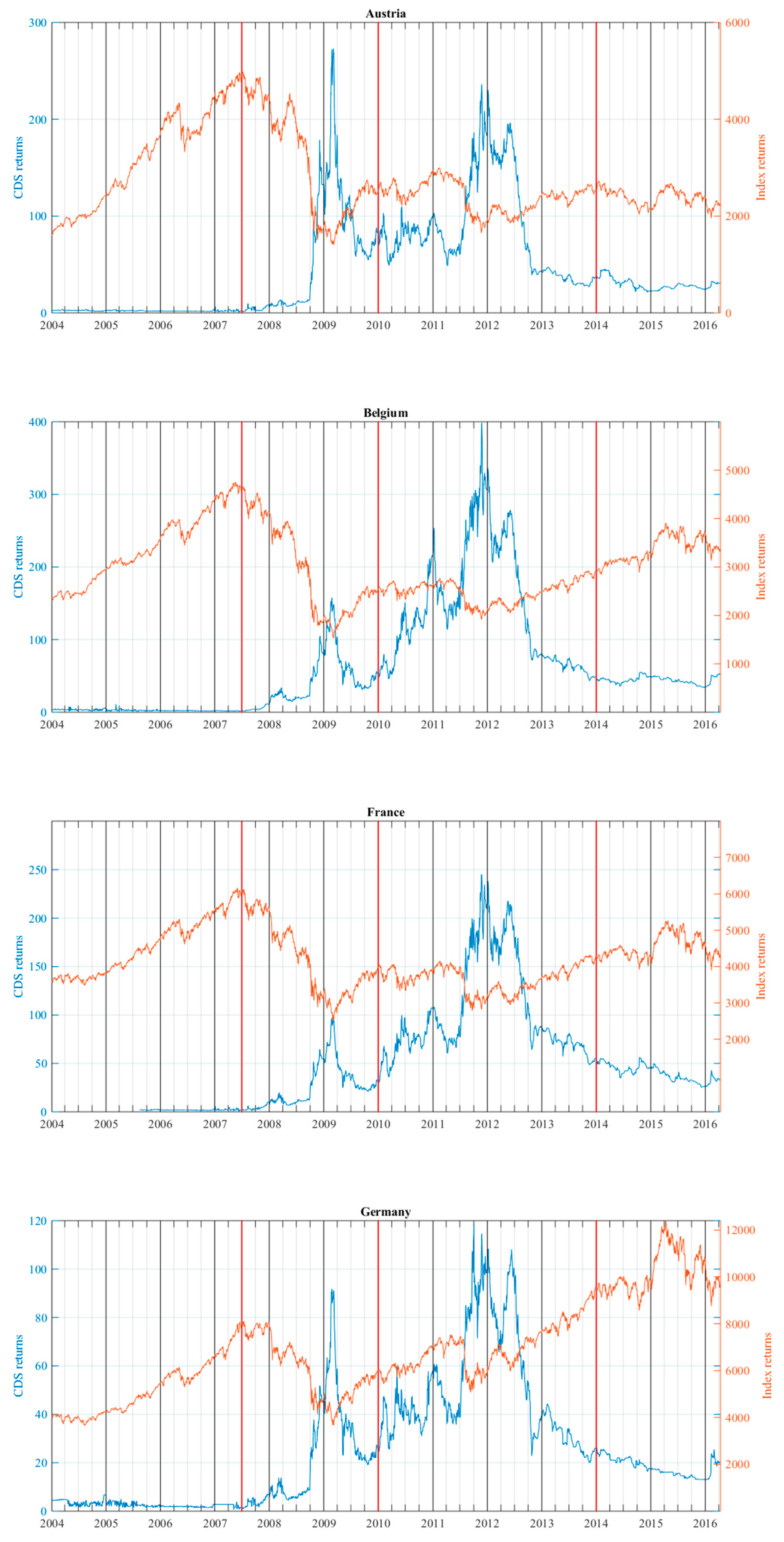
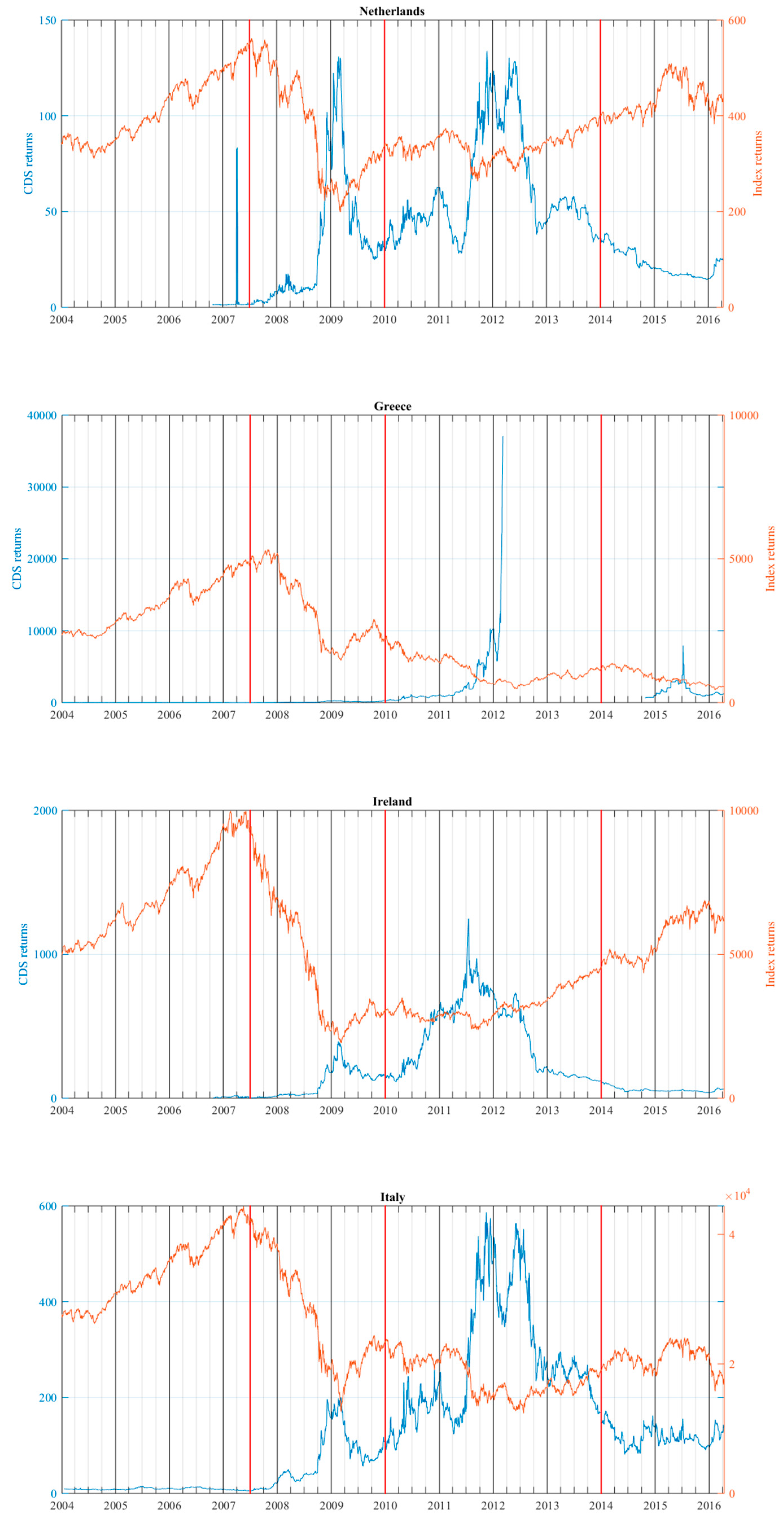
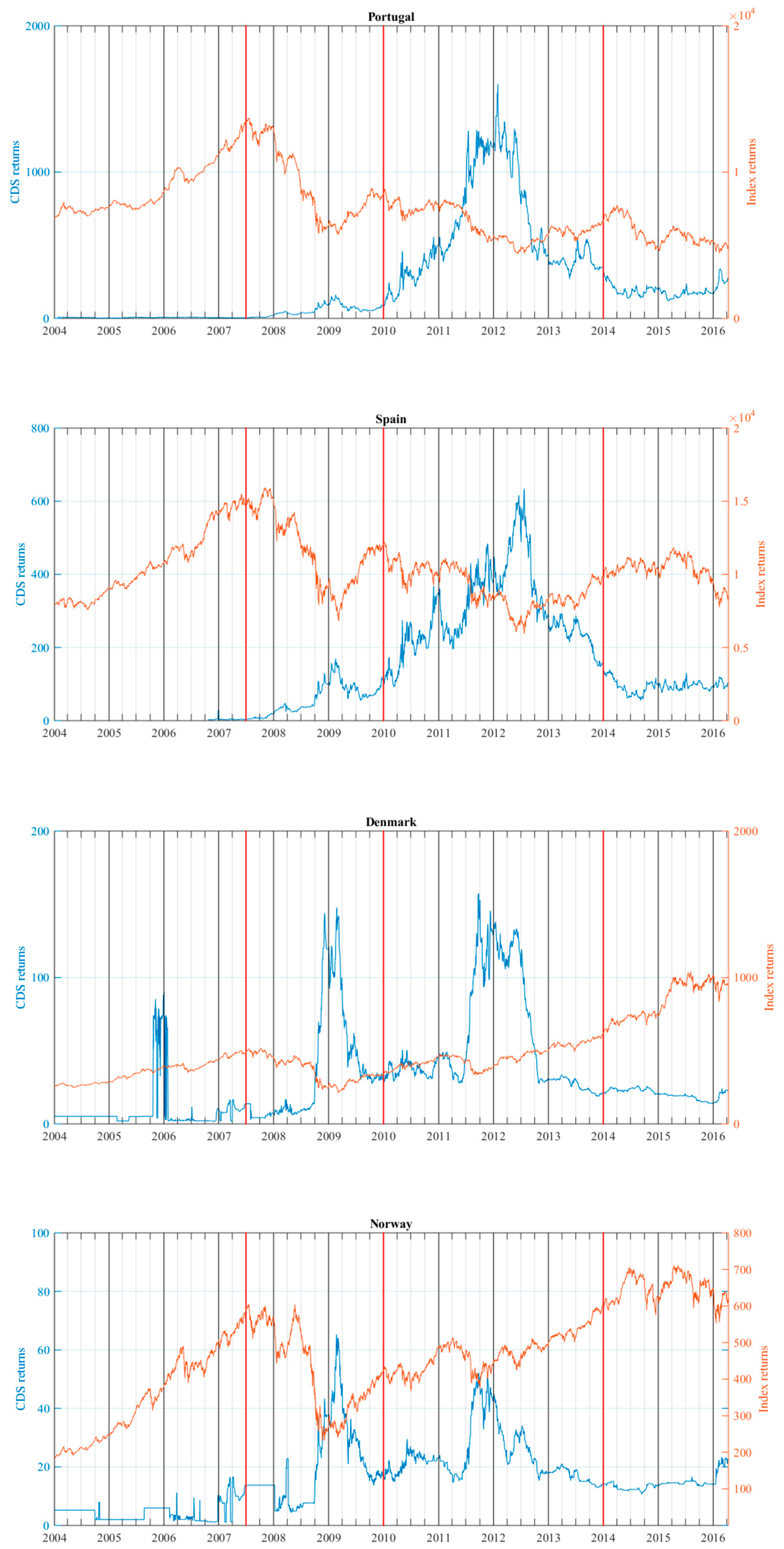
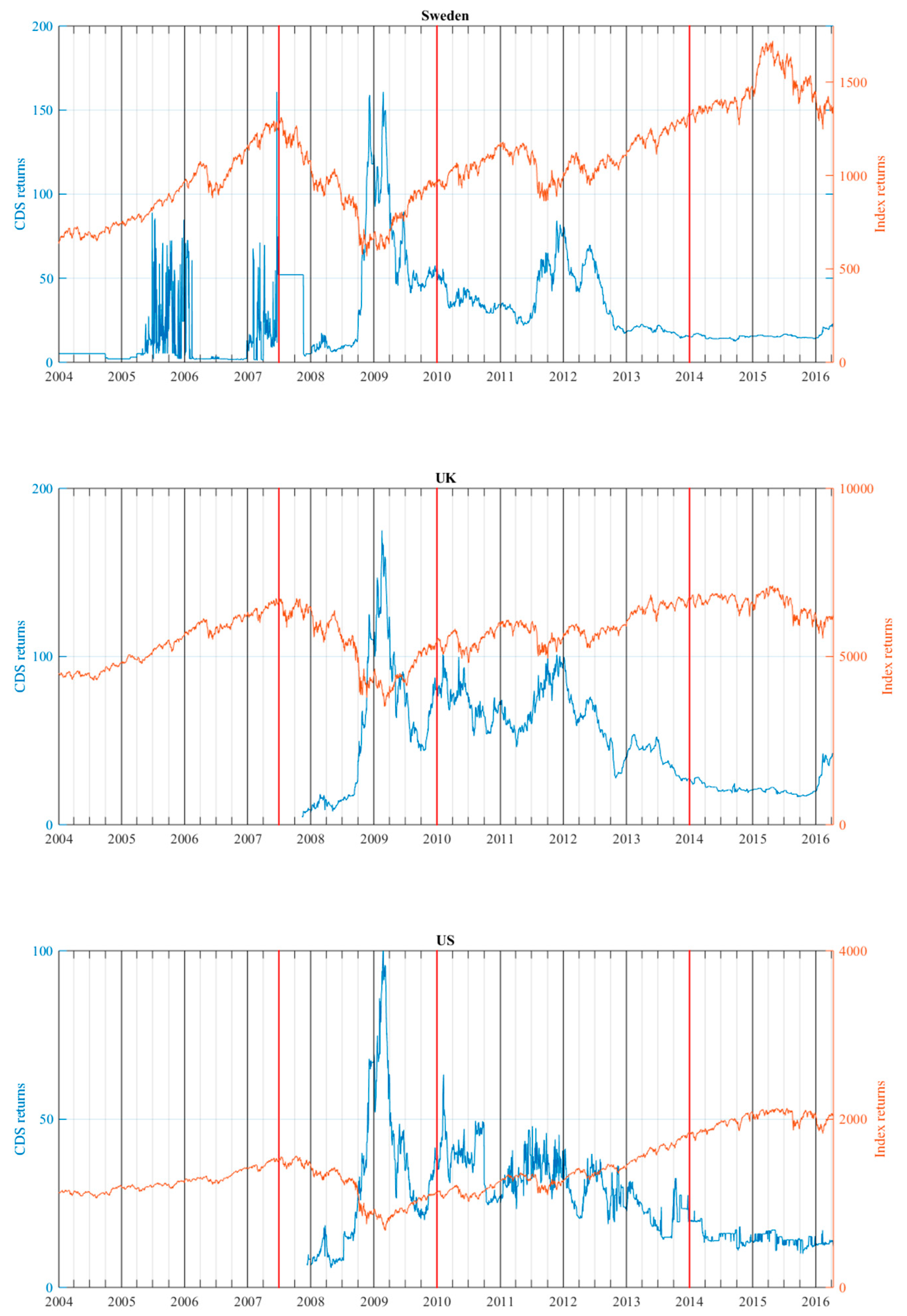
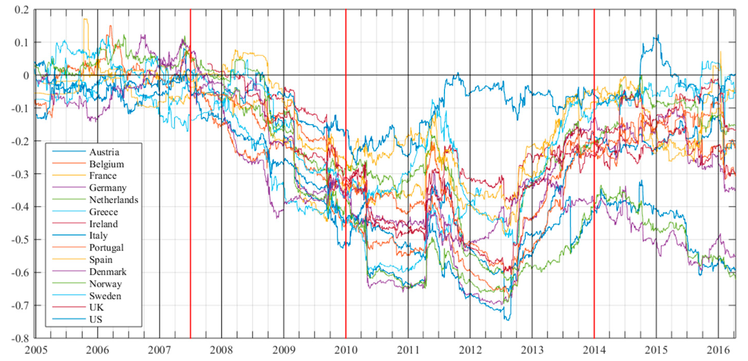
This table provides the descriptive statistics of sovereign CDS spreads and stock indices for European countries and the US. The sample period is from 6 January 2004 to 12 April 2016.

reports basic summary statistics for the stock indices and sovereign CDSs, while Figure 1 shows their daily time evolution during the sample period. CDS spreads differ substantially by country. What stands out is the distinction between non-Eurozone and Eurozone countries, and especially the differences among countries that belong to the Eurozone. In particular, it is noted that the Eurozone countries are divided into two main groups, justifying the distinction between Euro-peripheral and Euro-core countries. For instance, the means of Euro-peripheral sovereign CDSs range from 129.23 bps for Italy to 916.35 bps for Greece. In contrast, the means of Euro-core, non-Eurozone countries and US sovereign CDS spreads are considerably lower. In fact, the maximum level achieved in Belgium, the UK and the US amounts to 63.84, 48.94 and 26.51 bps, respectively. Focusing on some particular countries, we highlight the 37,081.41 bps maximum value of Greek sovereign CDSs (7 March 2012), due to the problems with the sovereign debt. Figure 1 also shows how a rise in credit risk, which is an increase in CDS spreads, is accompanied by a fall in the equity market, given that market risk also increases.

In order to capture the relative variation of the stock market index and the credit risk market, log-returns are calculated, for which certain statistical tests are carried out (we do not report these results to save space, but they are available upon request). The Jarque–Bera test rejects the normality of all the series, due to the excess of kurtosis and skewness. These results are indicative of non-normal distributions and fat tails, which are common features in financial series. Two different unit root tests are applied to check whether the credit spread series and stock returns series are non-stationary: the augmented Dickey–Fuller (ADF) test and the Phillips–Perron (PP) test. The results confirm that the hypothesis of non-stationarity is rejected, so the log-return series are stationary.

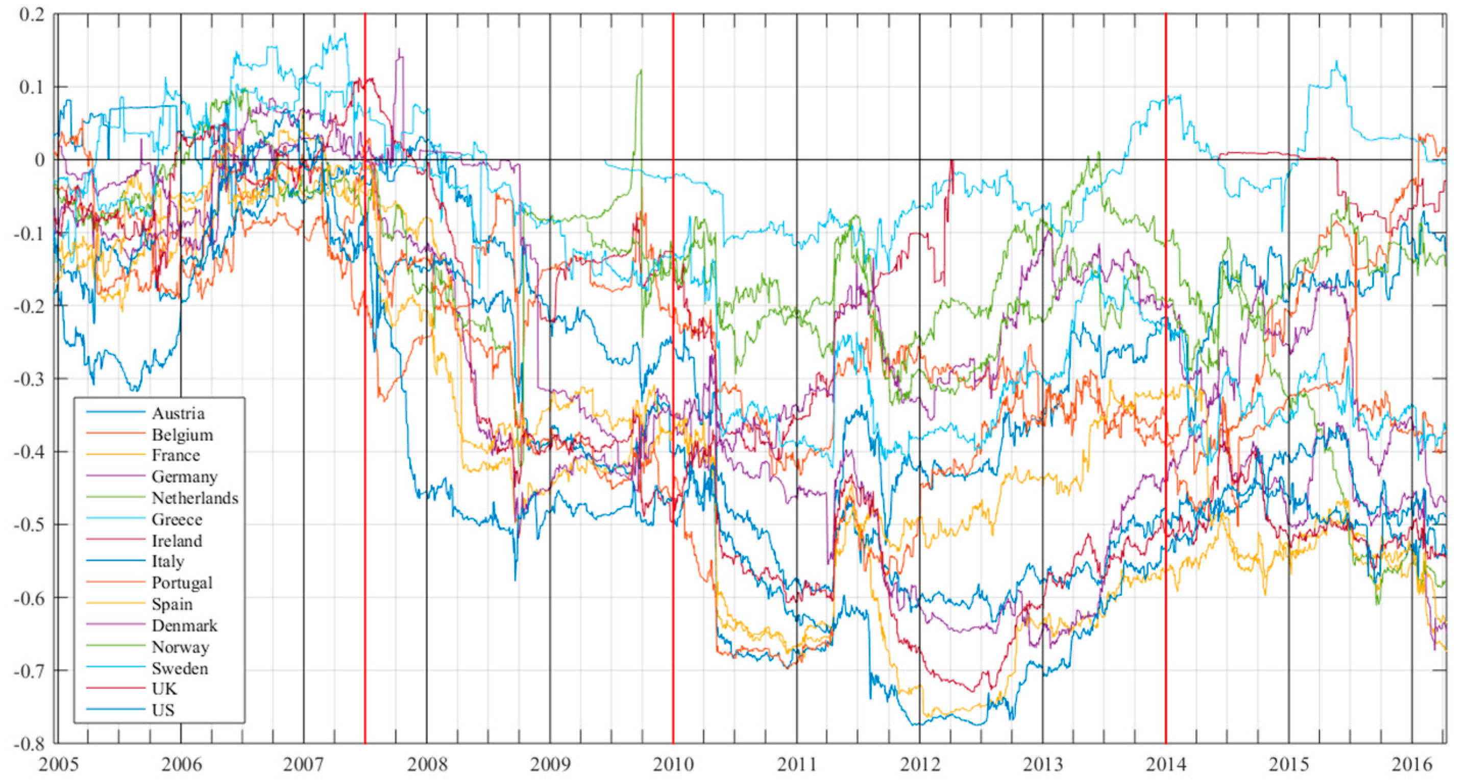
Figure 2 also shows the rolling inverse correlation dynamic for sovereign CDS and stock indices returns during the sample period. As typically occurs in periods of crisis, all the correlations in European markets increased considerably, with the maximum correlation levels (in absolute value) reached in the European sovereign debt crisis, especially affecting Italy, Portugal, Spain and Greece. These Euro-peripheral countries displayed the highest negative CDS–equity relationship values in this period. From 2012 to 2016, all European countries started to decrease the correlation levels with the exception of the cited Euro-peripheral countries. These preliminary results are in line with [18] for European sectoral iTraxx CDS indices. In particular, for the majority of the countries, the negative relationship is more pronounced during both the global financial crisis and the Eurozone sovereign debt crisis (mostly linked to Euro-peripheral countries).

4. Methodology

In this section, we analyse the interaction between stock and sovereign credit markets. In particular, we look for empirical evidence about the information flow between both markets, that is, we analyse if there is enough evidence on the anticipation of one market over the other. More concretely, the lead–lag relationship between the credit and stock markets is evaluated using the concept of Granger causality introduced by reference [24], and explained in depth in reference [25]. First, a bivariant vector autoregressive VAR(p) model is estimated for each of the 15 countries in the sample, using a similar methodology to previous studies, like [15] or [22], given by the following model:

$$\left[\begin{array}{c}{r}_{stock,t}\\ r_{CDS,t}\end{array}\right]=\left[\begin{array}{c}{\alpha }_{stock}\\ {\alpha }_{CDS}\end{array}\right]+{\displaystyle \sum }_{k=1}^p\left[\begin{array}{cc}{\beta }_{stock,stock,k}& {\beta }_{stock,CDS,k}\\ {\beta }_{CDS,stock,k}& {\beta }_{CDS,CDS,k}\end{array}\right] \left[\begin{array}{c}{r}_{stock,t-k}\\ r_{CDS,t-k}\end{array}\right]+\left[\begin{array}{c}{u}_{stock,t}\\ u_{CDS,t}\end{array}\right]$$

(1)

where $r_{stock,t}$ and $r_{CDS,t}$ are the stock indices and sovereign CDS log-returns considered and $u_{stock,t}$ and $u_{CDS,t}$ are the model error terms. The optimal VAR lag p for each country estimation has been chosen following the Akaike information criterion (AIC), the Schwarz Bayesian criterion (SBC) and the likelihood ratio test (LR) for the different lag lengths. In general, there is consistency between criteria, but when there is not, we follow the LR test in order to avoid over parametrization.

Next, we test if Granger causality exists between the stock index and the sovereign CDS, by imposing restrictions on the estimated coefficients. Specifically, if ${\beta }_{stock,CDS,k}=0$ for $k=1, 2\dots ,p$ in (1), we test the null hypothesis that the CDS market ($r_{CDS,t}$) does not Granger-cause the stock market ($r_{stock,t}$). If ${\beta }_{CDS,stock,k}=0$ for $k=1, 2\dots ,p,$ we test the null hypothesis that the stock market ($r_{stock,t}$) does not Granger-cause the CDS market ($r_{CDS,t}$).

As a novelty, we estimate the VAR model with a 250-observation time window in a rolling framework to identify the dynamic causal relationships between markets. We follow the authors of [26], who use a rolling 250-observation time window as an approximation of the number of trading days in a time horizon of one year. We verify the robustness of the results by modifying the size of the rolling window to 200 days (in line with [27] or [28]), both for the dynamic correlations and for the rolling causality analysis. If the traditional methodology provides two causality tests for the full sample period, with this approach we obtain, for each country and window, two series of p-values for both causality tests. Similar to [22], we employ these series in order to analyse graphically the direction of the causalities for the US sectoral market over time. However, we go one step further than their study. The two series of p-values obtained allow us to identify three transmission channels between the two markets considered, two unidirectional relationships (in a single direction) and one bidirectional transmission (in both directions). Specifically, we compute for each country the number of rolling windows (in percentage terms) in which a particular transmission is observed. The causality results for Europe are allocated into different groups computed as the average results by monetary zone (Eurozone and non-Eurozone) and for geographical zones within the Eurozone (Euro-peripheral and Euro-core). The idea is to contrast if there are significant differences pointing to a segmentation of the Eurozone between the countries most affected by the European sovereign debt crisis (Euro-peripheral countries) and the rest (Euro-core countries). Finally, we calculate these percentages for both the full sample period and after differentiating four important financial sub-periods: the pre-crisis period (January 2004–June 2007), the global financial crisis (July 2007–December 2009), the sovereign debt crisis (January 2010–December 2013) and the post-crisis period (January 2014–April 2016). In this way, we improve the conventional Granger causality estimations based on a static analysis for the whole sample period, studying whether the observed relationships vary over time.

5. Empirical Results: Lead–Lag Relationship between Stock Indices and Sovereign CDS Returns

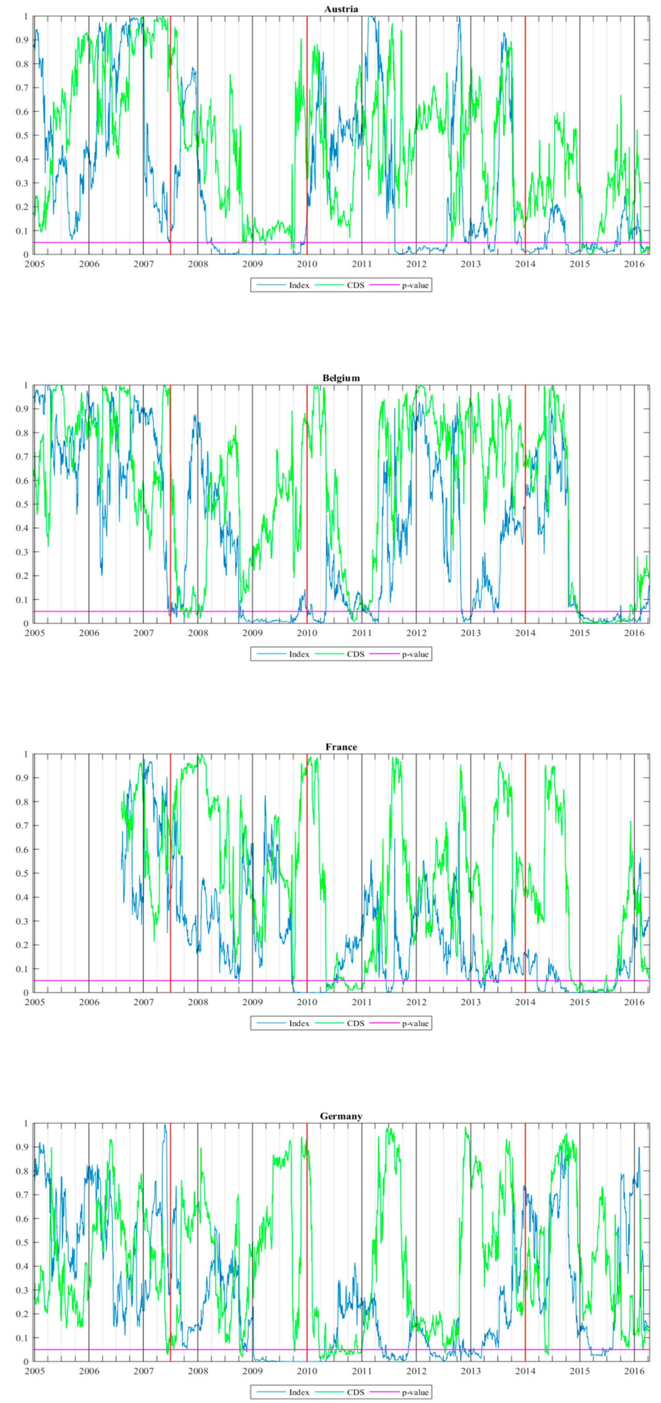
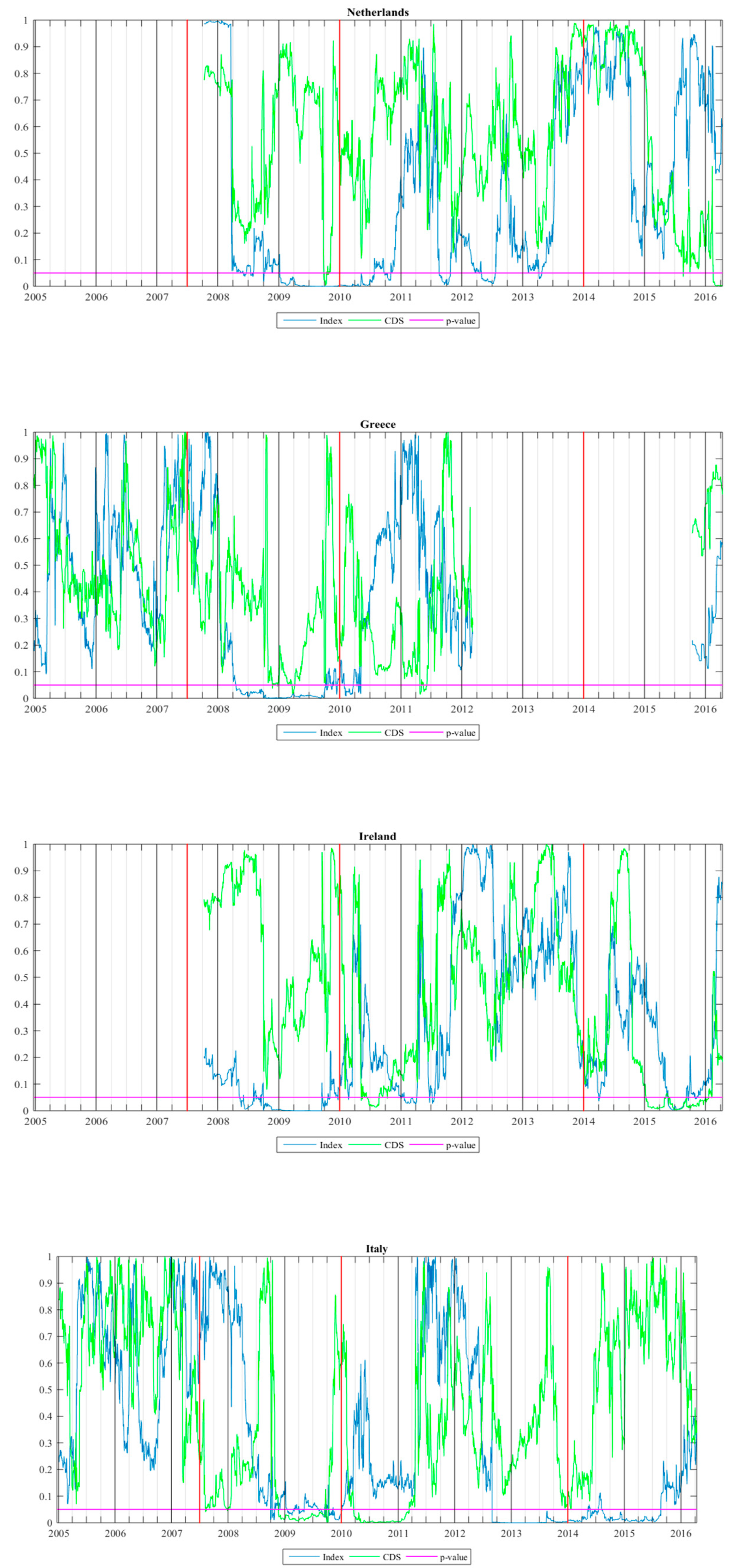
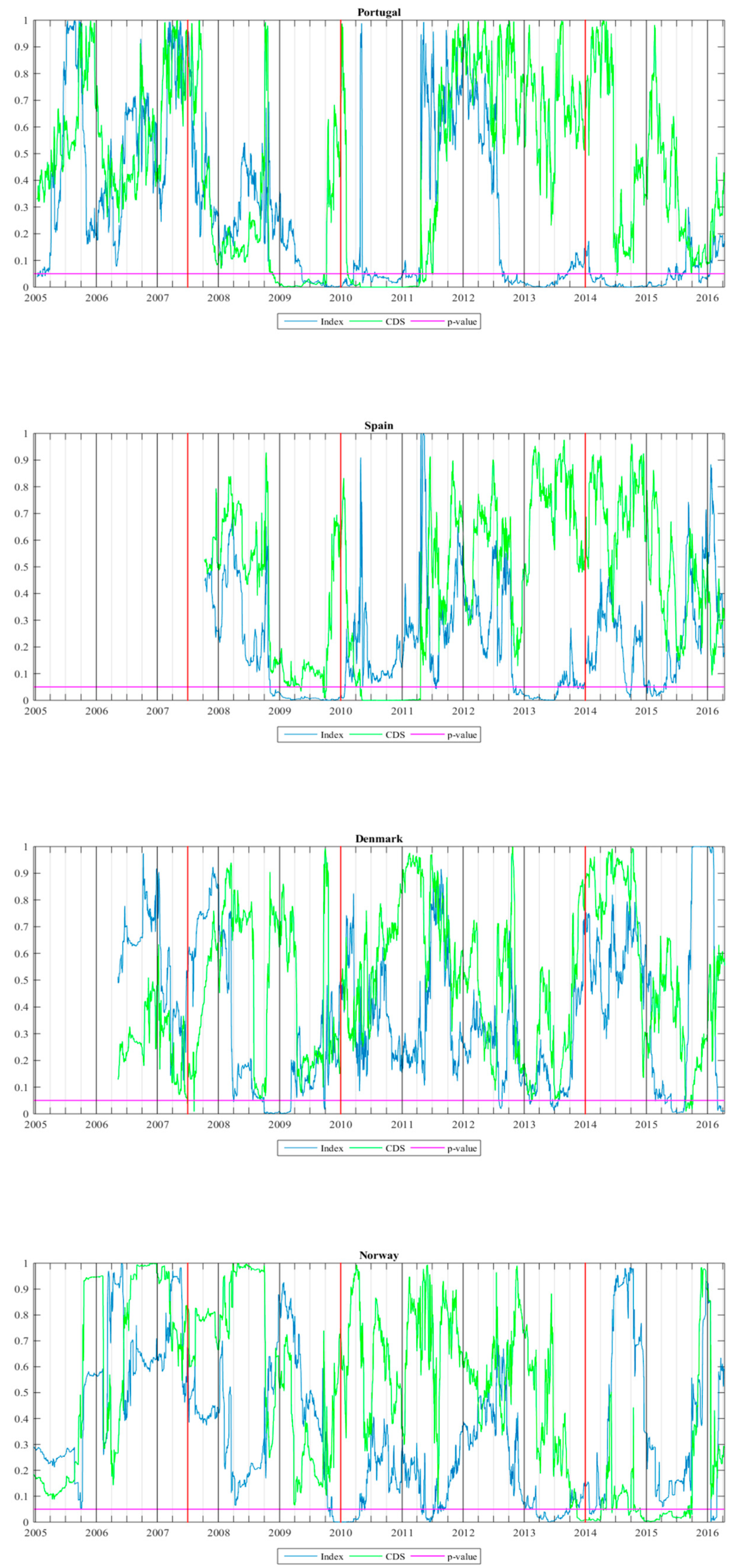
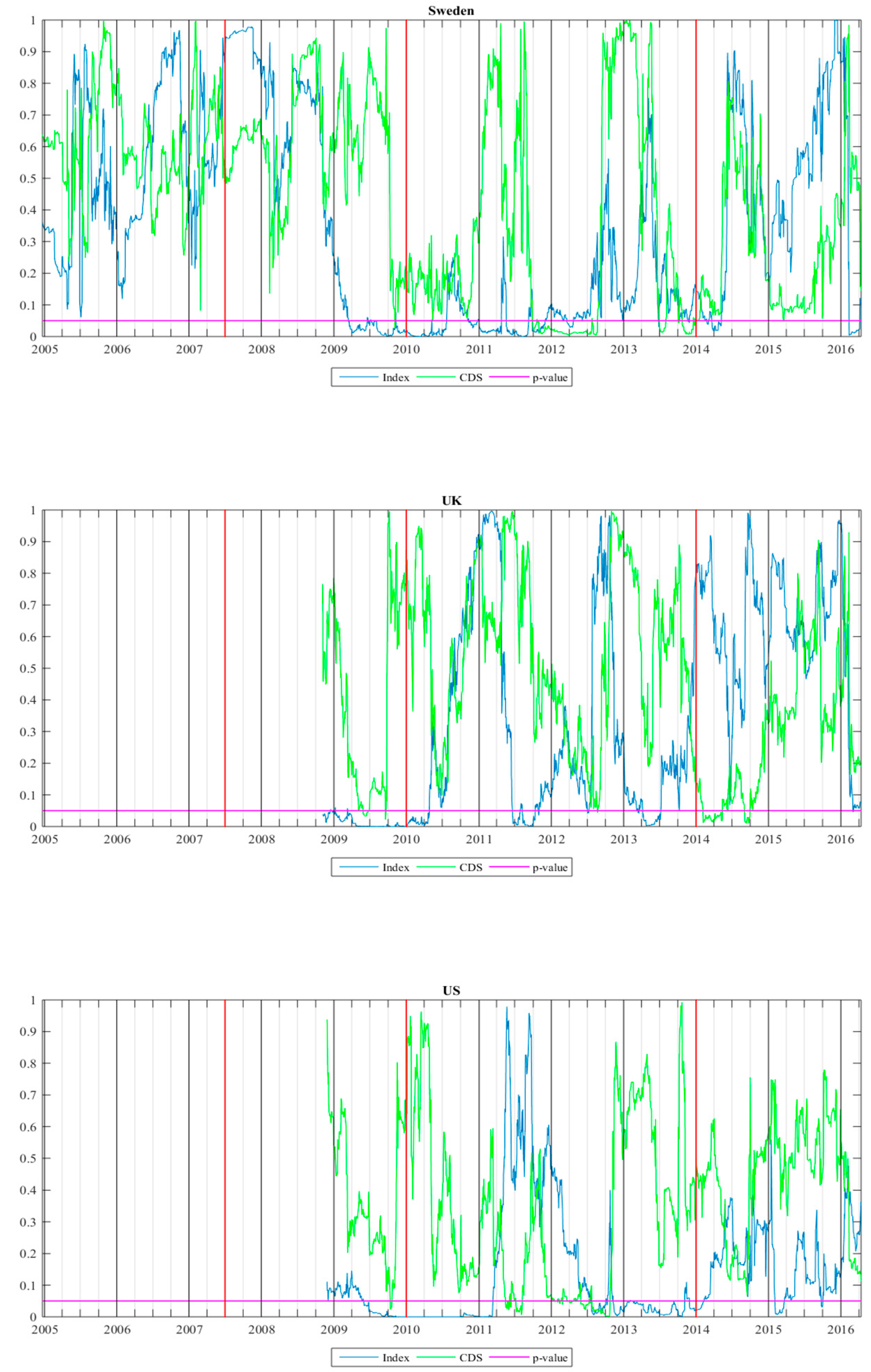
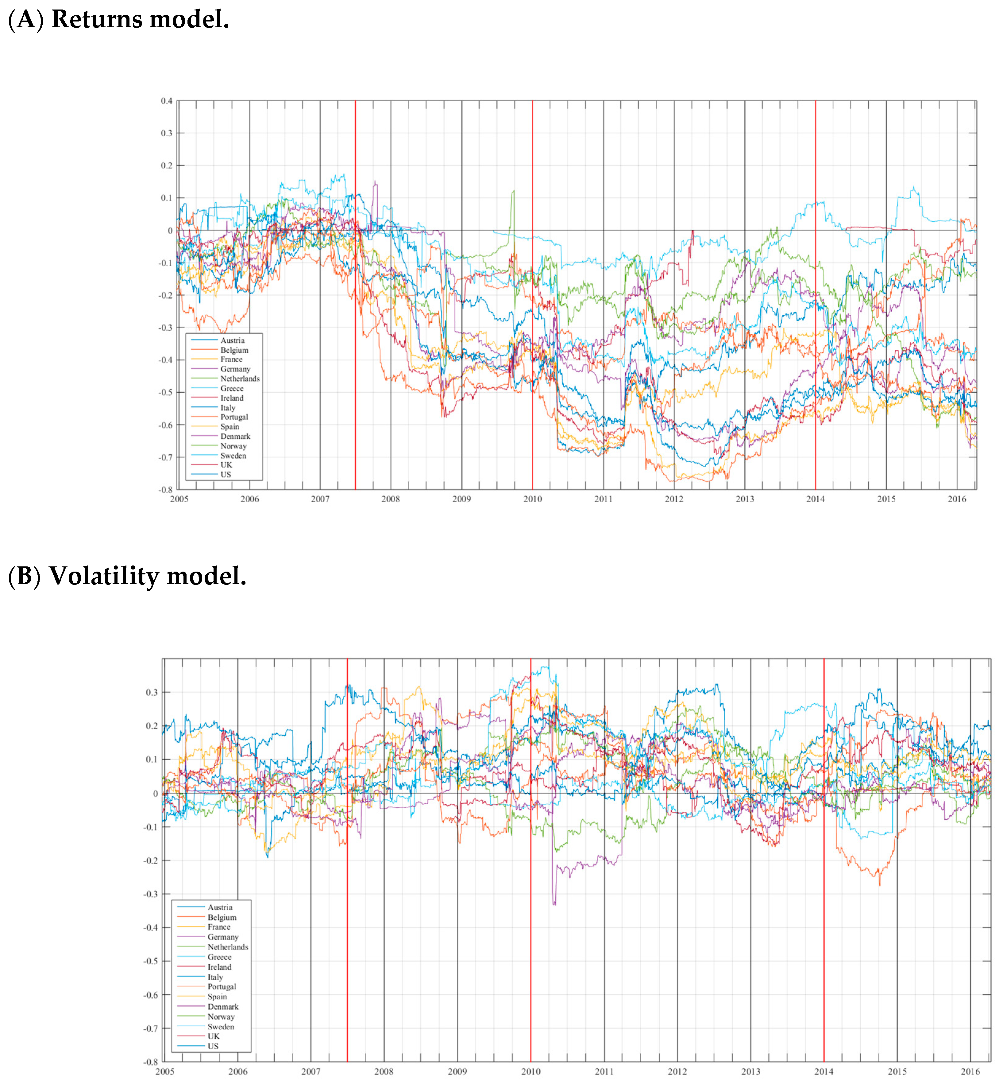
This section discusses whether there is enough empirical evidence to suggest that stock markets anticipate the CDS spread movements or vice versa. Figure 3 contains, for each country, the two series of p-values obtained for the causality test, as well as a line (in pink) indicating a significance level of 5%. When the p-value series in blue or green is below the pink line, this implies a significant causality relationship from stock to sovereign CDS or vice versa. Overall, the causalities between both markets are unstable and vary over time. There is a clear predominance of the stock market leading the CDS market, especially in times of crisis for all the countries; however, during the sovereign debt crisis we observe how the CDS market has increased its influence on the stock market in countries especially affected by this crisis, such as Italy, Portugal and Spain.

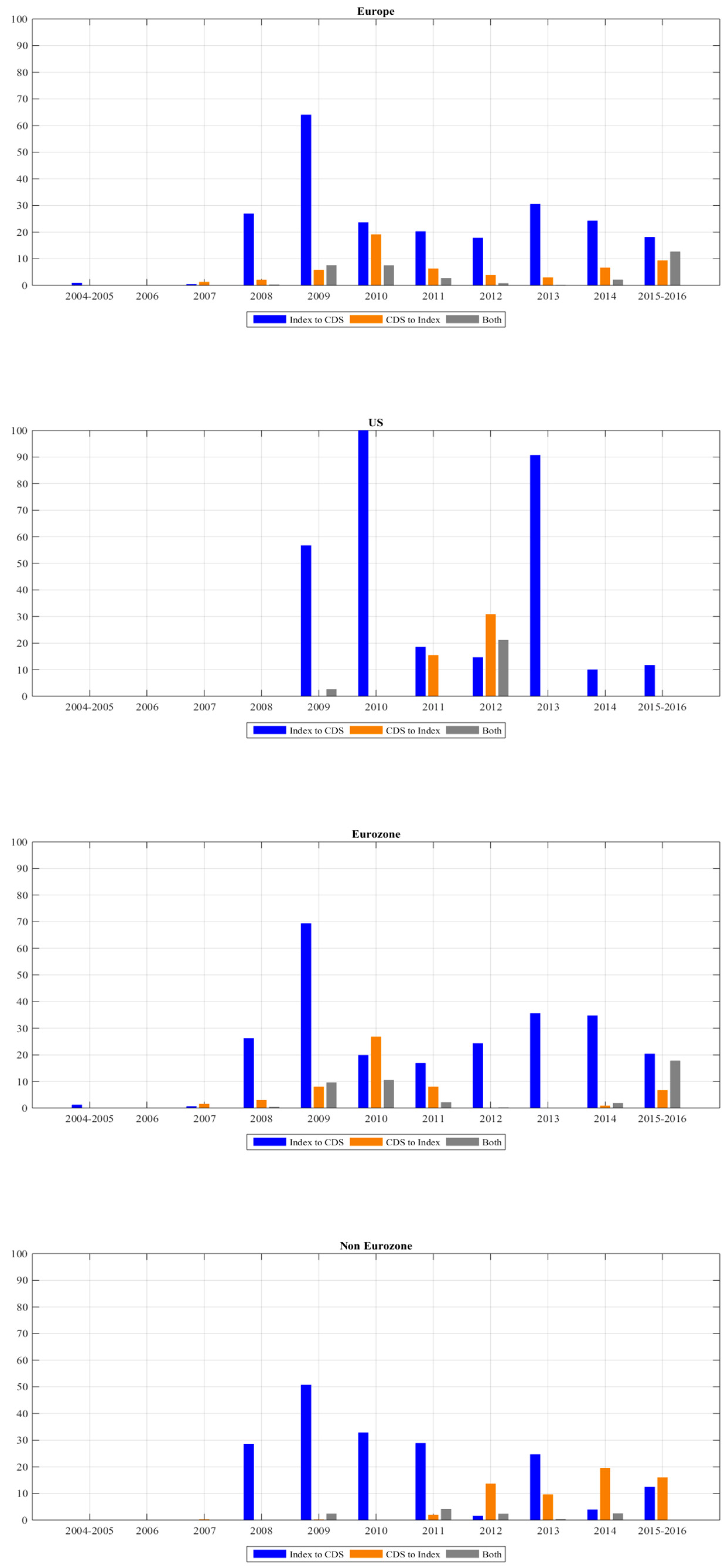
In order to quantify the directionality of results,

Table 2. Granger causality test results: stock indices and sovereign CDS returns.

	Full Sample January 2004–April 2016			Pre-Crisis January 2004–June 2007			Global Financial Crisis July 2007–December 2009			Sovereign Debt Crisis January 2010–December 2013			Post-Crisis January 2014–April 2016
Zone/Country	⇒	⇐	⇔	⇒	⇐	⇔	⇒	⇐	⇔	⇒	⇐	⇔	⇒	⇐	⇔
Austria	34.82%	0.24%	4.24%	0.00%	0.00%	0.00%	65.90%	0.00%	2.75%	30.01%	0.00%	0.00%	47.39%	1.18%	17.98%
Belgium	18.22%	2.41%	8.85%	0.91%	0.00%	0.00%	45.11%	5.81%	0.00%	17.74%	2.49%	1.15%	8.57%	1.18%	41.85%
France	15.28%	3.92%	9.54%	0.00%	0.00%	0.00%	11.01%	0.00%	0.31%	18.12%	9.49%	3.74%	21.01%	0.00%	33.61%
Germany	25.06%	4.96%	1.73%	0.00%	1.38%	0.00%	39.45%	1.99%	0.46%	37.78%	10.26%	4.60%	14.45%	2.86%	0.00%
Netherlands	25.83%	1.85%	0.77%	-	-	-	47.07%	0.00%	2.93%	28.76%	0.00%	0.00%	0.00%	6.89%	0.00%
Euro-core	23.84%	2.67%	5.03%	0.23%	0.34%	0.00%	41.71%	1.56%	1.29%	26.48%	4.45%	1.90%	18.29%	2.42%	18.69%
Greece	21.43%	1.14%	0.90%	0.00%	0.00%	0.00%	58.87%	0.00%	2.75%	8.07%	4.04%	0.00%	0.00%	0.00%	0.00%
Ireland	20.05%	10.23%	3.83%	-	-	-	62.82%	0.00%	0.00%	6.81%	5.27%	0.00%	1.51%	28.91%	14.29%
Italy	28.16%	13.84%	2.82%	0.00%	0.00%	0.00%	11.62%	23.24%	12.39%	33.56%	24.45%	0.00%	67.56%	0.00%	0.34%
Portugal	27.32%	7.25%	11.75%	2.95%	0.00%	0.00%	9.33%	18.96%	16.21%	28.76%	8.44%	22.82%	70.92%	0.17%	0.17%
Spain	27.17%	11.58%	0.81%	-	-	-	48.88%	0.00%	2.93%	22.15%	24.64%	0.10%	14.79%	0.00%	0.00%
Euro-peripheral	24.83%	8.81%	4.02%	0.98%	0.00%	0.00%	38.30%	8.44%	6.85%	19.87%	13.37%	4.58%	30.96%	5.82%	2.96%
Eurozone	24.33%	5.74%	4.52%	0.61%	0.17%	0.00%	40.01%	5.00%	4.07%	23.18%	8.91%	3.24%	24.62%	4.12%	10.82%
Denmark	10.74%	1.12%	0.00%	0.00%	0.34%	0.00%	19.42%	0.15%	0.00%	4.79%	0.00%	0.00%	16.97%	4.54%	0.00%
Norway	12.14%	11.16%	0.88%	0.00%	0.00%	0.00%	7.49%	0.00%	0.00%	27.23%	3.36%	0.00%	4.20%	49.41%	4.37%
Sweden	21.13%	7.93%	2.51%	0.00%	0.00%	0.00%	29.97%	0.31%	0.15%	33.37%	21.86%	7.00%	13.28%	0.67%	0.00%
UK	26.22%	4.84%	1.24%	-	-	-	89.11%	0.00%	7.92%	22.72%	0.19%	0.00%	0.34%	15.46%	0.00%
Non-Eurozone	17.56%	6.26%	1.16%	0.00%	0.11%	0.00%	36.50%	0.11%	2.02%	22.03%	6.35%	1.75%	8.70%	17.52%	1.09%
Europe	22.40%	5.89%	3.56%	0.39%	0.17%	0.00%	39.00%	3.60%	3.49%	22.85%	8.18%	2.81%	20.07%	7.95%	8.04%
US	41.58%	6.24%	3.22%	-	-	-	51.40%	0.00%	2.45%	56.18%	11.51%	5.27%	11.26%	0.00%	0.00%

This table shows the Granger causality test results by sub-periods between stock indices and sovereign CDS returns during the period 6 January 2004–12 April 2016. For each country and zone, we present the number of times (in percentage) that the null hypothesis of Granger causality is rejected. ⇒ indicates that the stock market causes the CDS market, ⇐ indicates that the CDS market causes the stock market and ⇔ indicates that both the stock market and the CDS market cause each other, reciprocally, in a given estimation window. (-) indicates the absence of data for this sub-period.

shows the number of causalities (in percentage) in which a particular transmission is observed, both for the entire period and for four sub-periods that include two financial crises (the global financial crisis and the European sovereign debt crisis) and two more stable periods that we call pre-crisis and post-crisis. In addition, for ease of discussion and to provide more information about the rolling transmission among the sub-periods, Figure 4 provides Granger causality results by year for US and European zones.

Results for the full sample period in Table 2 clearly show a unidirectional price discovery process from stocks leading CDSs. This general result is compatible with [8,14,20] for the US corporate market and [9,15] for the European firms and sovereign market. In addition, the impact of the transmission process is greater in the US than in Europe. Regarding the Eurozone and non-Eurozone countries, the information transfer is more intense in the case of the Eurozone. Inside the Eurozone, both geographical zones exhibit similar contribution percentages.

Sub-period analysis provides interesting results. While the causality relationship from the stock market to the CDS market is by far the most observed relationship, it is not the only one. The results show that at some specific moments, CDSs are in fact leading stocks, and even feedback processes or non-significant relationships are found. We also observe that the existence of lead–lag transmission is time varying and strongly linked to the economic cycle. In fact, it should be noted that this occurs only during the periods of crisis, both in Europe and the US, although in the case of the Eurozone it also occurs in the post-crisis period.

The absence of price discovery relationships in the pre-crisis sample is expected given the preliminary analysis of correlations. Before 2008, the relationship between both markets practically does not exist. This result is in line with what was previously found in the literature, except for [15,23]. In this regard, reference [23] document for European entities that during tranquil times, the CDS market’s contribution to price discovery is equal to or higher than that of the stock market. However, they use corporate data and stock market implied credit spreads instead of stock returns. In contrast, The authors of [15], with sovereign data, found that stocks lead the CDS market in tranquil times. Nevertheless, the authors consider the 2007–2009 period as a tranquil time because the objective is to analyse the European debt crisis in the year 2010. These conclusions should not be extrapolated to our paper due to the different data, methodology, sample and time periods and, in particular, crisis and non-crisis periods.

The significant causal relationships from stocks to CDSs are observed in the wake of the global financial crisis and the consequent European sovereign debt crisis. The leadership of the stock market affects all areas and countries, although with notable differences between the US and Europe. With values around 55% in both crises, the information transfer from stocks to CDSs is more intense in the US than in Europe, which shows a transmission of around 40% in the global financial crisis and about 20% in the European sovereign debt crisis, without significant differences between the different European monetary and geographical zones (see Table 2). Figure 4 shows that the maximum stock price discovery contribution in Europe is during 2009. In this year, the leadership of the stock market is strong due to the US financial crisis infecting Europe. This increasing effect during the subprime crisis is also observed in [9,10,23].

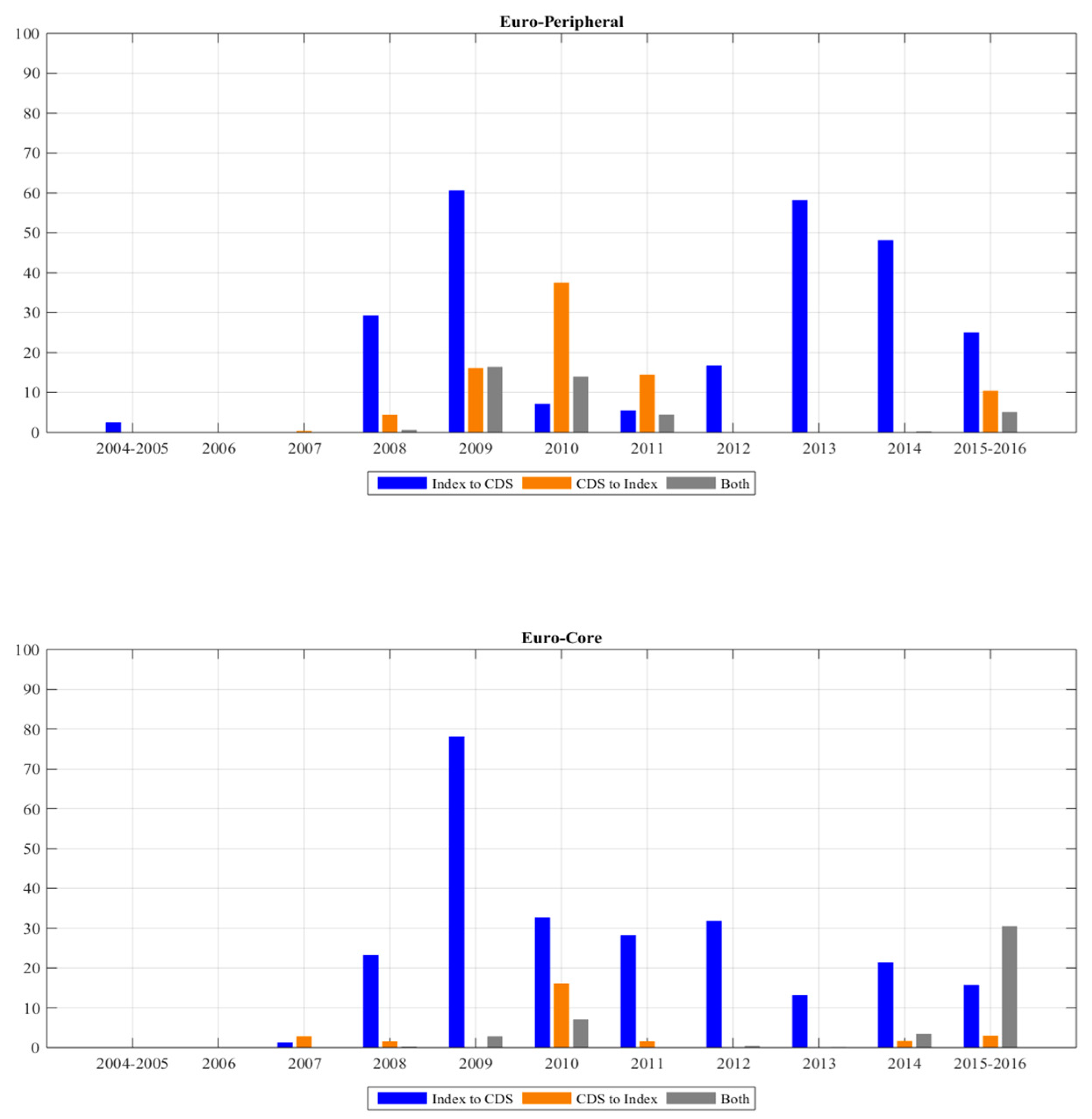
With the sovereign debt crisis, there is a change in the lead–lag trend in Europe and more specifically in the Euro-peripheral area. The stock returns are still leading, but not as evidently as before, as the CDS market has gained importance in Italy, Portugal and Spain. These peripheral countries were particularly affected by this crisis during 2010. Nevertheless, signs of instability appeared much earlier, as suggested by the causal relationship from CDSs to stocks observed since 2009 (Figure 3). According to [15], countries with high-risk spreads during the sovereign debt crisis are related to the transmission of CDS to stock returns. In addition, this result is in line with [22], who affirm that the corporate US CDS market leads its stock counterparts during the periods with significant credit events. The marked differences observed between the different European areas reveal the effects of the sovereign debt crisis in terms of the fragmentation of Europe. During 2011 and 2012, the causality relationships weakened in Europe, possible due to the adjustments made by European countries.

In the case of the US, we also observe several aspects to highlight during the Eurozone crisis. There are two large transmission peaks (over 90%) from stocks to CDSs in the years 2010 and 2013 (Figure 4). On the one hand, it seems that the problems experienced by the Eurozone in 2010 affected the US, increasing the transmission but maintaining the direction in the connection. On the other hand, the high transmission observed in 2013 coincides with the large bond market sell-off due to mortgage hedging trading in July 2013. Finally, 2011 and 2012 are the only years in which the CDS market increased its influence on the stock market in the US. In fact, in 2012, it is the causal relationship from CDSs to stocks that presents the greatest impact. The recovery in European countries may be behind the change in direction of the relationship.

The last years of the sample, which we have denominated the post-crisis period, were years of relative financial stability. As a consequence, the US and many of the European countries do not show significant causal relationships. However, two important facts should be highlighted in the case of the Eurozone. The bidirectional causal relationship found between markets in 2015, mainly due to Euro-core countries (specifically, Belgium and France), and the clear leadership of the stock market in the Euro-peripheral region, is exclusively due to the high transmission values of Italy and Portugal, countries that still faced serious debt problems during 2014 and early 2015 (see Figure 3).

6. Lead–Lag Relationship between Stock Return Conditional Volatility and Sovereign CDS Returns

Once the lead–lag relationship between the stock market and the CDS market in terms of returns is analysed, we consider the existence of a relationship for these markets based on volatilities. It is expected that the link between equity volatility and CDSs should be different than the equity–CDS returns link. The analysis in terms of volatilities has not been extensively explored to date. Some papers study this relationship, computing the volatility of the CDS spreads, but they get mixed results. The authors of [11,13] conclude that CDS market volatilities seem to lead stock market volatility, while reference [15] do not find evidence of a connection between stock volatility and the CDS market. However, in our approach, we do not compute CDS return volatility, as CDSs directly reflect the price of the credit risk. That is why we directly use CDS returns to analyse their relationship with the volatility of stocks. In this regard, we follow [12,14]. Both papers use data for US sectors, but with conflicting results. The former shows the leadership of the CDS market, while the latter finds a unidirectional causality from VIX to CDSs. Regarding this, more studies that analyse this relationship in terms of volatility are needed.

Specifically, we use stock conditional volatility to identify the relationship between stock return volatilities and CDS returns. It is important to note that stock return volatility must be previously obtained in order to estimate the VAR model (for further details, see Appendix A). Figure 5 shows the rolling correlation coefficients between stock volatility and CDS returns. As we expected, given the previous results in initial papers such as [18], correlations between variables are generally positive because both are risk measures, that is, if stock return volatility increases, sovereign credit risk also increases, represented by the rise in the CDS spread value.

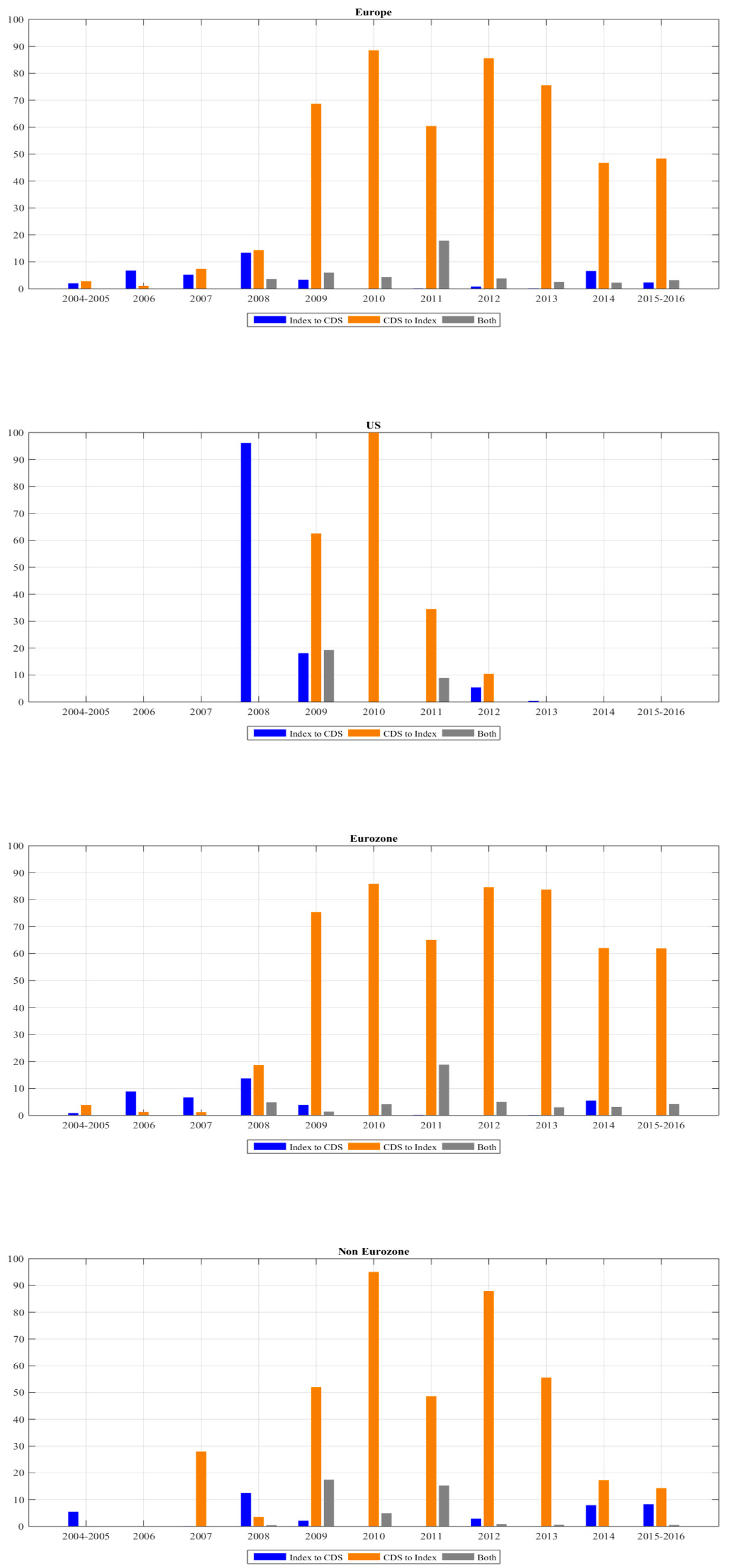
Following the same scheme as for the analysis of returns in the previous section, we begin by analysing the p-values obtained by performing the rolling test statistic, testing the null hypothesis that the conditional volatility of sovereign stock returns do not Granger-cause sovereign CDS returns or vice versa (figures for each country with the results of these tests are omitted to save space, but are available from the authors upon request). The existence of causal relationships is time varying and dependent on the crises in the financial markets. Nevertheless, contrary to what was obtained in the analysis of the lead–lag connections of returns, there is a clear predominance of CDS returns anticipating stock return conditional volatility.

Table 3. Granger causality test results: stock return volatility and CDS returns.

	Full Sample January 2004–April 2016			Pre-Crisis January 2004–June 2007			Global Financial Crisis July 2007–December 2009			Sovereign Debt Crisis January 2010–December 2013			Post-Crisis January 2014–April 2016
Zone/Country	⇒	⇐	⇔	⇒	⇐	⇔	⇒	⇐	⇔	⇒	⇐	⇔	⇒	⇐	⇔
Austria	6.18%	50.92%	4.82%	1.38%	0.00%	0.00%	5.81%	35.32%	0.00%	0.48%	88.49%	7.38%	21.85%	58.15%	10.92%
Belgium	0.00%	67.83%	1.53%	0.00%	7.94%	0.00%	0.00%	72.17%	0.00%	0.00%	95.69%	4.31%	0.00%	80.17%	0.00%
France	4.91%	58.92%	9.06%	20.00%	0.00%	0.00%	11.77%	31.35%	2.91%	0.00%	79.67%	20.13%	0.00%	76.13%	0.00%
Germany	4.07%	44.38%	0.34%	4.75%	0.00%	0.00%	13.61%	32.42%	0.00%	0.00%	98.08%	0.96%	0.00%	12.10%	0.00%
Netherlands	4.73%	65.93%	2.34%	-	-	-	18.07%	33.56%	2.93%	0.00%	96.64%	3.36%	0.00%	43.70%	0.00%
Euro-core	3.98%	57.60%	3.62%	6.53%	1.98%	0.00%	9.85%	40.96%	1.17%	0.10%	91.72%	7.23%	4.37%	54.05%	2.18%
Greece	5.22%	1.64%	0.05%	6.72%	0.00%	0.00%	9.02%	4.74%	0.00%	0.35%	0.35%	0.18%	0.00%	0.00%	0.00%
Ireland	5.99%	43.76%	1.89%	-	-	-	20.83%	16.87%	0.00%	0.00%	62.42%	1.15%	2.02%	37.31%	5.04%
Italy	0.00%	60.37%	11.50%	0.00%	5.25%	0.00%	0.00%	67.43%	0.00%	0.00%	70.76%	29.24%	0.00%	94.45%	5.55%
Portugal	0.48%	60.93%	10.69%	0.00%	0.00%	0.00%	1.22%	55.96%	19.27%	0.58%	89.55%	9.20%	0.00%	82.18%	15.46%
Spain	0.00%	83.24%	0.99%	-	-	-	0.00%	39.59%	0.17%	0.00%	97.99%	2.01%	0.00%	100.00%	0.00%
Euro-peripheral	2.34%	49.99%	5.03%	2.24%	1.75%	0.00%	6.21%	36.92%	3.89%	0.19%	64.21%	8.36%	0.40%	62.79%	5.21%
Eurozone	3.16%	53.79%	4.32%	4.39%	1.87%	0.00%	8.03%	38.94%	2.53%	0.14%	77.96%	7.79%	2.39%	58.42%	3.70%
Denmark	8.19%	31.84%	2.55%	0.00%	0.00%	0.00%	17.43%	22.32%	7.95%	2.88%	58.77%	0.67%	11.43%	10.92%	1.18%
Norway	0.07%	27.20%	0.00%	0.00%	0.00%	0.00%	0.00%	14.83%	0.00%	0.00%	66.92%	0.00%	0.34%	1.18%	0.00%
Sweden	1.26%	44.61%	1.73%	4.43%	13.44%	0.00%	1.22%	59.79%	0.00%	0.00%	77.47%	4.89%	0.00%	4.71%	0.00%
UK	7.37%	63.01%	15.56%	-	-	-	6.93%	24.75%	44.22%	0.00%	83.89%	16.11%	20.50%	45.88%	0.00%
Non-Eurozone	4.22%	41.66%	4.96%	1.48%	4.48%	0.00%	6.40%	30.42%	13.04%	0.72%	71.76%	5.42%	8.07%	15.67%	0.29%
Europe	3.46%	50.33%	4.50%	3.73%	2.66%	0.00%	7.57%	36.51%	5.53%	0.31%	76.19%	7.11%	4.01%	46.21%	2.73%
US	4.73%	28.10%	3.79%	-	-	-	25.78%	56.45%	17.42%	1.63%	36.34%	2.21%	0.00%	0.00%	0.00%

This table shows the Granger causality test results by sub-periods between stock index volatilities and CDS returns during the period 6 January 2004–12 April 2016. For each country and zone, we present the number of times (in percentage) that the null hypothesis of Granger causality is rejected. ⇒ indicates that stock market volatility causes the CDS market, ⇐ indicates that the CDS market causes stock market volatility and ⇔ indicates that both cause each other, reciprocally, in a given estimation window. (-) indicates the absence of data for this sub-period.

provides, both for the full sample and for the four sub-samples considered, the number of times (in percentage) in which a particular causality is observed, while Figure 6 collects these percentages by year in order to offer more information about the rolling transmission.

Results for the full sample period of Table 3 are in line with [12] and clearly show the leadership of CDS returns anticipating stock volatility. This is the first major difference from the model in returns: the causality changes direction and, while stock returns caused CDS returns, now it is the CDSs that cause the volatility of the shares. Moreover, the intensity of the price discovery is once again different in Europe and the US. Notably, the leadership of CDSs is stronger for Europe. This is the second difference (at least for the entire sample) since it used to be the US that had more causal relationships. Within Europe, the transmission is slightly higher for the Eurozone than for the non-Eurozone, and also somewhat higher in the Euro-core zone than in the Euro-peripheral zone.

The analyses by sub-samples show interesting results. In line with the findings in terms of returns, we only find significant causality relationships in Europe and the US for the two crisis periods, and in the post-crisis period for the Eurozone. The pre-crisis period is a period of financial stability during which no causal relationships are observed between the two markets, either considering equity returns or equity volatilities. It is from the global financial crisis that a clear causal relationship between CDS returns and equity volatilities is observed, although with different characteristics depending on the sub-period and the geographical area.

During the global financial crisis, Europe experienced an increase in the connection between markets, with CDS returns anticipating the volatility of stock market indices. This pattern was more evident in Eurozone countries than in non-Eurozone countries, and within the former, Euro-core countries exhibited greater causality compared to Euro-peripheral countries. The US displayed a different causality behaviour. The outbreak of the subprime crisis was characterised by the opposite one-way relationship in which the volatility of shares led the CDS market, with 2008 being the only year in which this direction is observed in causality. In 2009, the relationship followed the trend in Europe, displaying, as in the rest of the sample, an apparent causality of CDS returns towards volatility in the stock market.

During the European debt crisis, the growing trend of CDSs leading stock market volatility continued in Europe, with the maximum contribution level of the sample being reached in 2010 (with values of almost 90% in average terms). Looking at the entire sub-period, there are no significant differences between the various monetary zones, confirming that with respect to volatilities, the fragmentation of Europe in terms of returns is not observed. However, it is within the Eurozone where the Euro-core countries experience a higher causality ratio than the Euro-peripheral ones. Additionally, for the US, 2010 is characterised as the year with the highest transmission peak (100%) and, as in the case of Europe, transmission is from CDS returns to stock index volatility. Over the next few years, the connection noticeably decreases until it no longer exists in the post-crisis period.

In the case of Europe, causality behaves differently during the post-crisis period. The levels of connection between the two markets decreased notably compared to the previous sub-period, although CDSs continued to dominate share volatility, with the Eurozone countries being the only ones that registered significant transmissions.

The analysis in terms of volatilities reveals some interesting results that add value to the analysis in returns. We observe that there is a change in the direction of the market transmission, a change that is due to the dynamic in the equity market. It is important to remember that we use CDS returns in both analyses. On the other hand, the geographic area leadership is also different. We note that when using returns (volatilities), a greater contribution is attributed to the US (Europe). Furthermore, the causality percentages obtained in the volatility analysis for all European countries are much higher than those obtained with returns. For the US, our findings are in line with the corporate US contagion study in [12], where contagion in returns is greater than the volatility spillovers.

7. Additional Analysis: Lead–Lag Relationship between Bank Stock Indices and Bank CDS Indices

In addition to sovereign data, we employ financial stocks and CDS data in the analysis. Following the spirit of [11,21], we believe that the vulnerability of European financial institutions is still an important fact, largely due to the large amount of sovereign debt they possess and to their role as a financial instability connector to the whole system. Consequently, the concerns about the solvency or credit risk of the banking systems have increased. The objective of this analysis is to check if a lead–lag relationship exists between financial stocks and CDSs and also if this connection is similar to our previous sovereign results.

Financial stock index data are obtained from Datastream, who build country-specific banking indices using the most representative banks in each country. In particular, Datastream computes sectoral indices as follows. For each market, a representative sample of stocks covering a minimum of 75–80% of total market capitalization enables market indices to be calculated. By aggregating market indices for regional groupings, regional and world indices are produced. Within each market, stocks are allocated to industrial sectors using the Industry Classification Benchmark (ICB) jointly created by FTSE and Dow Jones.

Additionally, CDS spreads for banks located in the previous countries are collected. Following [28], only banks with actively traded CDS data over the period are selected. The financial sector reference entities include the largest share of the actively traded CDSs. For the empirical analysis, we exclude some banking firms due to the availability of updated data in Reuters.

Table 4. List of European and US banks.

Country	Bank Name	Obs.	Country	Bank Name	Obs.
Eurozone			Euro-Peripheral (Continued)
Euro-core (14)			Portugal (2)	Banco Espirito Santo	3201
Austria (2)	Erste Group Bank	3201		Banco Comercial Português	3201
	RaiffeisenZentralbank	3201	Spain (5)	Banco Santander	3201
Belgium (1)	KBC Bank	3201		Banco Bilbao Vizcaya Argentaria	3201
France (5)	BNP Paribas	3201		Banco Popular Español	3201
	Société Générale	3201		Banco de Sabadell	2293
	Crédit Agricole	3201		Bankinter	2801
	Natixis	3201	Non-Eurozone (12)
	BPCE SA	3201	Denmark (1)	Danske Bank	3191
Germany (4)	Deutsche Bank	3201	Norway(1)	DNB NOR ASA	2069
	Commerzbank	3201	Sweden (4)	Nordea Bank	3201
	Deutsche Postbank	3177		Svenska Handelsbanken	3201
	HSH Nordbank	3201		Skandinaviska Enskilda Banken	3201
Netherlands (2)	ING Bank NV	3201		Swedbank	3091
	Rabobank	3201	UK (6)	HSBC Holdings PLC	3201
Euro-peripheral (16)				Lloyds Banking Group	3201
Greece (2)	National Bank of Greece	1712		Alliance and Leicester PLC	2887
	Alpha Bank	3201		Barclays	3201
Ireland (1)	Allied Irish Banks	2173		Royal Bank of Scotland Group	3201
Italy (6)	Unicredito Italiano	3201		HBOS	3201
	Banca Monte Paschi Siena	3201	US (3)
	Unione di Banche Italiane	3161		Bank of America corporation	3201
	Banco Popolare	3199		JP Morgan Chase & Co	3201
	Banco Popolare Milano	3201		Citigroup Inc.	3201
	Banca Italease	2313

This table shows the European and US banks used to build the financial CDS index. Banks are assigned to countries based on the Datastream classification. Obs. refers to the available number of observations (CDS spread) for each bank in the sample.

illustrates the list of European and US banks. The sample is composed of 45 large banks, 42 European banks and 3 US banks. Finally, based on the iTraxx and banking stock index structure, an equally weighted banking CDS index is constructed for each country. More specifically, our financial sample is composed of 100,264 unbalanced panel observations for 3201 days.

Table 5. Main descriptive statistics of daily financial stock indices and bank CDS spreads.

	Financial CDS					Financial Stock Indices
Country	Obs.	Min.	Max.	Mean	Std. Deviation	Obs.	Min.	Max	Mean	Std. Deviation
Eurozone
Euro-core
Austria	3201	3.83	510.25	124.62	85.33	3201	153.83	896.27	433.51	175.40
Belgium	3201	6.90	511.10	117.65	106.24	3201	76.32	1877.74	691.61	551.32
France	3201	5.18	356.17	90.32	74.67	3201	191.75	1149.65	554.74	230.31
Germany	3201	10.22	276.11	91.47	58.55	3201	88.84	676.98	291.54	150.50
Netherlands	3201	3.40	214.67	66.94	50.90	3201	98.91	5007.18	1401.87	1578.62
Euro-peripheral
Greece	3201	10.80	3876.74	607.09	694.60	3201	0.47	3312.48	1101.71	1056.58
Ireland	2173	63.50	1812.99	696.54	571.10	3201	40.54	8549.14	2364.49	2810.52
Italy	3201	9.78	706.50	180.78	158.01	3201	338.70	3169.15	1385.72	762.65
Portugal	3201	8.10	1615.18	298.77	341.72	3201	9.41	352.16	111.05	89.50
Spain	3201	8.33	700.77	173.69	170.10	3201	138.68	566.35	319.83	103.19
Non-Eurozone
Denmark	3191	1.00	344.80	83.06	78.47	3201	696.82	4839.75	2646.84	897.47
Norway	2071	37.50	212.00	85.76	36.90	3201	130.46	1056.76	593.65	178.14
Sweden	3201	9.63	242.38	67.18	50.74	3201	891.87	4343.30	2560.61	703.93
UK	3201	4.10	298.86	88.61	68.03	3201	1663.32	9649.60	5242.71	2253.32
US	3201	8.67	421.06	98.65	74.71	3201	282.86	1889.44	1110.52	411.97

This table provides the descriptive statistics of financial CDS spreads and stock indices for European countries and the US. The sample period is from 6 January 2004 to 12 April 2016.

shows the basic summary statistics for the financial stock indices and CDS. In the same way as in the sovereign case, financial CDS spreads vary by country. The highest CDS spreads are found in Euro-peripheral countries, while the lowest values are observed in the non-Eurozone countries. For instance, the minimum average levels were achieved in Sweden (67.18 bps), Denmark (83.06 bps) and Norway (85.76 bps). Nevertheless, with a value of 37,081.41 bps, Greek banks show the maximum CDS value, closely followed by Ireland and Portugal, reflecting the lack of solvency of Greek, Irish and Portuguese banks during the European sovereign debt crisis.

Similarly to the procedure followed with the sovereign sector, we compute the rolling correlations between financial CDS returns and financial stock returns and conditional volatilities. The estimation parameters of the conditional volatility model for financial stock returns and the figures for each country are omitted to save space, but are available from the authors upon request. Likewise, although we omit the results related to the statistical tests for reasons of space, as expected, financial stocks and CDS returns series are stationary.

Figure 7 shows the results of the rolling correlations. We observe a stronger negative correlation for the financial returns, which could be indicating a stronger lead–lag relationship between the stock and the CDS markets in the banking sector compared to the sovereign sector. In addition, it is observed that financial stock return volatility shows slightly higher levels than sovereign return volatility and the correlation coefficients are higher during crisis periods.

Next, we analyse the p-values of the rolling analysis for financial stocks and CDS returns and volatilities (figures for each country with the rolling causality results are available upon request).

Table 6. Granger causality test results: bank indices and bank CDS returns.

	Full Sample January 2004–April 2016
	Return Model			Volatility Model
Zone/Country	⇒	⇐	⇔	⇒	⇐	⇔
Austria	45.39%	3.90%	17.58%	0.86%	41.08%	3.14%
Belgium	50.34%	2.47%	2.00%	2.88%	38.69%	1.36%
France	28.72%	4.75%	1.46%	0.85%	75.17%	5.09%
Germany	27.62%	1.39%	1.05%	3.16%	65.56%	7.57%
Netherlands	16.58%	8.92%	1.70%	0.68%	19.57%	1.93%
Euro-core	33.73%	4.29%	4.76%	1.68%	48.01%	3.82%
Greece	13.38%	13.51%	0.00%	6.28%	14.83%	0.12%
Ireland	27.52%	0.00%	0.00%	20.46%	0.89%	11.62%
Italy	47.12%	2.98%	1.90%	0.92%	72.84%	6.00%
Portugal	23.22%	2.24%	9.05%	2.78%	42.66%	4.44%
Spain	44.31%	3.93%	0.00%	0.00%	68.33%	1.56%
Euro-peripheral	31.11%	4.53%	2.19%	6.09%	39.91%	4.75%
Eurozone	32.42%	4.41%	3.47%	3.89%	43.96%	4.28%
Denmark	25.57%	0.74%	1.48%	7.60%	21.63%	0.00%
Norway	54.40%	0.05%	0.49%	1.70%	49.34%	10.93%
Sweden	41.06%	1.25%	7.97%	3.90%	46.02%	1.93%
UK	19.04%	3.97%	0.68%	0.10%	58.69%	9.88%
Non-Eurozone	35.02%	1.51%	2.66%	3.33%	43.92%	5.69%
Europe	33.16%	3.58%	3.24%	3.73%	43.95%	4.68%
US	37.46%	6.54%	13.76%	0.27%	79.28%	8.55%

This table shows the Granger causality test results between bank indices and bank CDS returns during the period 6 January 2004–April 12 2016. For each country and zone, we present the number of times (in percentage) that the null hypothesis of Granger causality is rejected. 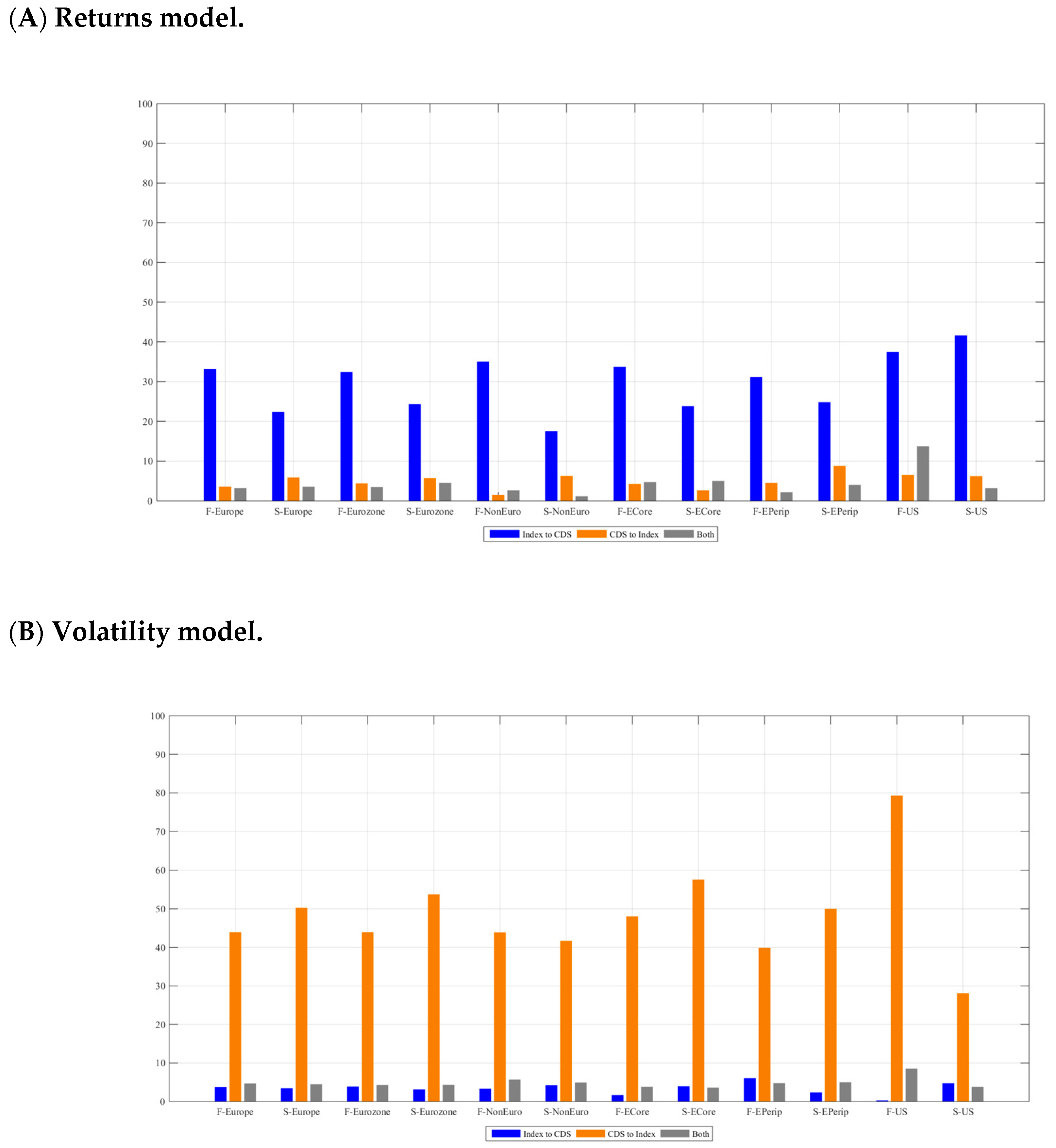⇒ indicates that the stock market causes the CDS market, ⇐ indicates that the CDS market causes the stock market and ⇔ indicates that both the stock market and the CDS market cause each other, reciprocally, in a given estimation window.

offers, for the case of the banking sector and the full sample, the number of causalities (in percentage) for each country and geographical area considered. In addition, for ease of discussion, Figure 8 shows the comparative results of the information transfer relationships between both sectors.

In line with the findings obtained for the sovereign sector, there is clear leadership of the equity market over the CDS market in terms of returns (same result as [21]) and the opposite relationship in volatilities, with CDS returns causing equity volatilities (consistent with [11]). However, there are some peculiarities depending on the sector and the analysis considered. On the one hand, although the price discovery contribution from stocks to CDS returns is still stronger for the US, the difference compared to Europe is not so marked. In fact, the US shows a slightly lower percentage for the financial sector and a much higher one in the case of Europe, especially in the non-Eurozone. This means that, in the financial sector, the contribution of causality in the analysis of returns is similar in Europe and the US (in contrast to [11], who observe a greater impact in the case of European banks). On the other hand, the impact of the transmission process of financial CDS returns on stock volatilities is somewhat lower compared to the sovereign sector in the Eurozone, but significantly higher in the US. Therefore, the leadership of CDS returns causing stock volatilities is stronger in the sovereign (banking) sector for Europe (US).

8. Conclusions

The objective of the study is to use a rolling VAR model to analyse in terms of returns and volatilities the transmission dynamics between the stock and the CDS markets. Given the scant prior evidence in this regard, we consider sovereign and financial daily data from January 2004 to April 2016 for 14 European countries and the US. The long sample period allows us to analyse the impact that crises of a different nature, such as the global crisis of 2008 and the Eurozone debt crisis, have had on the mechanisms of information transmission between the two markets. Our goal is to understand how financial crises are formed and transmitted, which can be useful in the face of financial distress events that may occur in the future.

The findings for the sovereign sector reveal that, regardless of whether the analysis is in returns or volatilities, the price discovery contribution of both markets is time varying and is dependent on the economic cycle. Causality only occurs during bad economic times, both in Europe and the US, although in the case of some Eurozone countries, it is also found in the post-crisis period.

We find that the stock market clearly leads the CDS market in terms of market returns. This result is consistent for both the sovereign and banking sectors, and it is more intense in the US than in Europe, although the difference is not so marked in the financial case. In general, no significant differences are observed between the different European monetary and geographical zones. However, with the sovereign debt crisis, the fragmentation within Europe becomes evident. The stock returns are still leading, but not as evident as before, as the sovereign CDS market has gained importance in Italy, Portugal and Spain, countries that were particularly affected by this crisis during 2010.

Regarding the volatility model results, the causality changes direction, as we find evidence that CDS returns are able to anticipate what happens to stock market volatility, for the sovereign and banking sectors in the US as well as in Europe. From a sovereign perspective, CDS leadership is stronger in Europe than in the US, and also greater in Eurozone countries than in non-Eurozone countries. In contrast, a greater impact is observed in the US than in Europe with respect to the financial sector, but surprisingly we do not find significant differences within Europe.

In short, we conclude that the transmission process between the credit and equity markets exists. We confirm that stock returns anticipate CDS returns, and that the latter anticipate the conditional volatility of stock returns, showing a returns and volatilities connection channel between the markets. An important result is that the transmission between markets is more intense or less intense in one or another geographical area depending on the sample period, the sector considered and whether the analysis is in terms of returns or volatilities.

These results are especially useful in terms of understanding the dynamics of risk transmission; knowledge about correlations and the price discovery process between markets should be taken into consideration by portfolio managers in order to match assets in optimal portfolios. Another important issue to take into account is the development of appropriate strategies related to hedging credit derivatives with stocks, the analysis of portfolio performance and comparing portfolio results in turbulent and tranquil periods. Furthermore, we have identified that more studies with respect to volatilities are needed. Finally, it would also be interesting to analyse the connection not only between markets within the same country but also among a sample of different samples.