Fractional Dynamics and Pseudo-Phase Space of Country Economic Processes

Abstract

In this paper, the fractional calculus (FC) and pseudo-phase space (PPS) techniques are combined for modeling the dynamics of world economies, leading to a new approach for forecasting a country’s gross domestic product. In most market economies, the decline of the post-war prosperity brought challenging rivalries to the Western world. Considerable social, political, and military unrest is today spreading in major capital cities of the world. As global troubles including mass migrations and more abound, countries’ performance as told by PPS approaches can help to assess national ambitions, commercial aggression, or hegemony in the current global environment. The 1973 oil shock was the turning point for a long-run crisis. A PPS approach to the last five decades (1970–2018) demonstrates that convergence has been the rule. In a sample of 15 countries, Turkey, Russia, Mexico, Brazil, Korea, and South Africa are catching-up to the US, Canada, Japan, Australia, Germany, UK, and France, showing similarity in many respects with these most developed countries. A substitution of the US role as great power in favor of China may still be avoided in the next decades, while India remains in the tail. The embedding of the two mathematical techniques allows a deeper understanding of the fractional dynamics exhibited by the world economies. Additionally, as a byproduct we obtain a foreseeing technique for estimating the future evolution based on the memory of the time series.

1. Introduction

The last crisis (2007–2008) was severe, and it came without adequate warning to markets and policymakers. High unemployment rates could not be avoided, and the austerity programs had enormous impacts on standards of living, and caused extensive suffering. While sound democracies have been implanted in the Western world, sacrifice associated with austerity throughout the 2008 financial crisis could not be alleviated, and great discredit has befallen economics as a social science.

The use of gross domestic product (GDP), and GDP per capita, to assess economic performance and prosperity has long been discussed. The indicator does not include any out-of-market production, as self-consumption escapes accounting efforts and methods altogether. At the same time, negative externalities of economic growth, such as inequality, resource depletion, pollution, environmental degradation, and effects on climate, have been forgotten, although they always affect future economic growth [1].

The claim for better prosperity indicators and welfare measurement includes political fears about the capacity of democratic political regimes to implement them [2]. While there are no better metrics to reflect people’s lives and aspirations that will be able to inspire better policies for better lives after the 2008–2009 crisis, the US and the European economies have been growing slightly more slowly than in earlier years, according to GDP metric.

As slower economic growth has been coupled with urban riots, strikes, warring, and mass migrations around the world, analysts have been led to doubt the possibility of overcoming social problems. Pessimistic views from Fogel 2007 even discuss the US capacity to go on performing as the world great power [3]. They predict an acceleration of convergence, and suggest that by 2040 the world may experience a global geopolitical turnover related with the relative economic decline of the US. Beyond alternative techniques to be invented to measure prosperity, the relative share of the US GDP in the global GDP will fall from 22% to 14%, according to Fogel [3]. For Europe, the relative share of the European GDP in the global GDP will fall from 21% to 5%, it is said.

The contrast of post-war prosperity with post 2007–2008 crisis is evident. Social, political, and military conflicts, including urban riots, terrorism, guerrilla actions, and outright warfare, are afflicting all continents and regions of the world. Independently of the construction of other indicators to assess economic performance and social progress, as suggested by Stiglitz et al. [1], the successful catching-up of Asian partners to core countries, coupled with their expansionary demography, will bring about fear for the survival of democracy, as this will depend on the political options of those Asian countries, according to Fogel.

Experts have recalled other aspects related with past crisis indicators, and concluded that the ongoing crisis has a new scale in comparison with any others in the past: Banking systems in Europe have faced episodes of instability several times in the nineteenth and twentieth centuries, but those crises were much less severe. The new millennium has brought monetary policies based on low interest rates that do not compensate for individuals’ saving efforts, which is consistent with the ongoing banking crisis and the financial instability, which have increased in this period [4,5,6,7].

From the perspective of market economies, crises are normal episodes. Modern markets in capitalism have developed frequent episodes of booms and busts [8]. Surely, booms mean prosperity (sometimes with bubbles) and give origin to busts (or even crises, recessions, and depressions), that historically were followed by new prosperity [9]. Marxian views on the end of capitalism never materialized [10]. The failure of the less-adapted firms during crises can explain Capitalism’s resilience and survival (until now). Business cycles alternating between prosperity and crisis are intrinsic features of market economies.

Independently of the invention of new measures for human welfare and happiness, economic convergence of national economies deserves generalized approval, because, in improving the lowest standards of living around the world, convergence contributes to global welfare.

In the 1960s Alexander Gerschenkron, economic historian at Harvard, devoted his attention to economic growth in a historical perspective, and identified the meaning of industrialization for prosperity to recall the higher rates of economic growth in the late-comers. According to Gerschenkron’s hypothesis, the adoption of new technologies commands industrialization, helping imitators to grow faster [11]. This observation from the post-WWII perspective is remarkable, even if governments assumed strong roles in national economies. In many countries, such as France or the UK, the government’s policies did not stimulate capital markets in the 1950s and 1960s because of nationalization of important sectors of economic activity [12]. However, the American role in joining European countries to the Marshall Plan offer in the OEEC, in 1948, guided them to considerable co-operation, putting Western partners into an openness attitude towards global capital markets, again.

The 1948–1973 period experienced the most successful economic growth of the entire history of humankind. It allowed the defeated Japan and late-industrialized countries to catch up to the developed European countries. Genuine economic modernization and urbanization occurred [13]. Individual aggressive competitive behavior was extended to more traditional societies. Co-operation with governments in strategies of growth, which included the formation of conglomerates and cross-participation of multinational firms, provided safety and more robust opportunities in Asian markets. In adopting new technologies for productive investment, Asian countries were successful in catching-up with the most-developed nations. A convergence process took place in each country in industrialization.

Fractional calculus (FC) is a mathematical formalism that models efficiently phenomena with non-locality and long term memory. On the other hand, the pseudo-phase space (PPS) is a tool for studying dynamics while avoiding the calculation of derivatives. Recently, various authors applied the tools of classical dynamical systems to the economy. Petráš and Podlubny [14] used the state space for describing national economies, while adopting GDP, inflation, and unemployment rates as state variables. Machado and Mata [15,16] analyzed the Economic and Monetary Union countries and their similarities during the integration process, and investigated the Portuguese short-run business cycles over the last 150 years, using the multidimensional scaling method for visualizing the results. Škovránek et al. [17] proposed an approach to macroeconomic modeling based on the state space, fractional-order differential equations, and orthogonal distance fitting. The GDP, inflation, and unemployment rates were adopted as state variables. Machado and Mata [18] presented a bond-graph approach to model economy. The generalization of the principle of conservation of power and the assignment of causalities were circumvented by means of a variable fractional-order element. Machado et al. [19] investigated the economic growth using the multidimensional scaling method and state space portrait analysis. The GDP per capita was adopted as the main indicator for economic growth and prosperity, and the long-run perspective from 1870 to 2010 for identifying the main similarities among countries’ economic growth. Machado and Mata [20] proposed the PPS and FC for modeling the Western global economic downturn. Tarasova and Tarasov [21] introduced a generalization of the economic model of logistic growth by considering the effects of memory and crises. The memory effects are modeled with fractional order derivatives. Using the equivalence of fractional differential equations and the Volterra integral equations they obtained discrete maps with memory that were exact discrete analogs of fractional differential equations of economic processes. Tarasov and Tarasova [22] designed a model of economic growth with fading memory and continuous distribution of delay time. Their approach can be considered as a generalization of the standard Keynesian macroeconomic model. Tejado et al. [23] presented models of economic growth for the countries of the Group of Seven (G7) for the period 1973–2016. Such models consisted of differential equations of both integer and fractional order, where the GDP was a function of the country’s land area, arable land, population, school attendance, gross capital formation, exports of goods and services, general government final consumption expenditure, and broad money. Ming et al. [24] applied the Caputo fractional derivative to simulate China’s GDP growth, while comparing the effectiveness of both fractional and integer order models. Škovránek [25] proposed a mathematical model based on the one-parameter Mittag–Leffler function to describe the relation between the unemployment and the inflation rates, known as the Phillips curve. For a comprehensive literature review see [26] and the references therein.

Hereafter, the aforementioned questions are analyzed using the FC and PPS in the scope of the complex dynamics of world economies and the perspective of 15 important countries. Furthermore, a new approach for forecasting the GDP is proposed. The common adoption of the two approaches leads to (i) a clear visualization and a straightforward interpretation of the dynamic effects, and (ii) foreseeing the future dynamics of the time series (TS). The 15 selected countries are Australia, Brazil, Canada, China, France, Germany, India, Japan, Korea, Mexico, Russia, South Africa, Turkey, the United Kingdom, and the United States.

The paper has the following organization. Section 2 introduces the fundamentals of the FC and the PPS representation. Section 3 develops the methodology and the analytical formulation for studying the dynamics of the TS. Section 4 discusses the proposed estimators and evaluates their efficiency. Finally, Section 5 summarizes the conclusions.

2. Fundamental Concepts

2.1. The Fractional Calculus

The FC generalizes the derivative of a function f, $D^{\alpha }f\left(x\right)$, to orders $\alpha \in \mathbb{R}$ [27,28]. During the last decades FC has become a popular tool [29,30,31], and new areas of application have emerged. The modeling finance [32] and economy [18,21,22,26,33,34,35] phenomena became of particular relevance.

The Riemann–Liouville and Caputo are classical definitions of a fractional derivative (FD), being given by [36]:

$${\displaystyle {}_a^{RL}{\mathcal{D}}_t^{\alpha }x\left(t\right)=\frac{1}{\mathsf{\Gamma }(n-\alpha )}\frac{{\mathrm{d}}^n}{\mathrm{d}{t}^n}{\int }_a^t\frac{x\left(\tau \right)}{{(t-\tau )}^{\alpha -n+1}}\mathrm{d}\tau ,n-1<\alpha <n,}$$

(1)

$${\displaystyle {}_a^C{\mathcal{D}}_t^{\alpha }x\left(t\right)=\frac{1}{\mathsf{\Gamma }(n-\alpha )}{\int }_a^t\frac{x^{\left(n\right)}\left(\tau \right)}{{(t-\tau )}^{\alpha -n+1}}\mathrm{d}\tau ,n-1<\alpha <n,\alpha >0,}$$

(2)

where $\mathsf{\Gamma }\left(·\right)$ denotes the gamma function and $\{t,a\}\in \mathbb{R}$ ($t>a$) are the upper and lower limits of the calculation interval, respectively.

Another classical expression is the Grünwald–Letnikov (GL) definition. The GL formulation has the advantage of leading to a straightforward digital implementation and is given by [36]:

$${}_a^{GL}{\mathcal{D}}_t^{\alpha }x\left(t\right)=\underset{h\to 0^{+}}{lim}\frac{1}{h^{\alpha }}\sum _{k=0}^{\left[\frac{t-a}{h}\right]}\gamma \left(\alpha ,k\right)x\left(t-kh\right),t>a,\alpha >0$$

(3a)

$$\gamma \left(\alpha ,k\right)={\left(-1\right)}^k\frac{\mathsf{\Gamma }\left(\alpha +1\right)}{k!\mathsf{\Gamma }\left(\alpha -k+1\right)},$$

(3b)

so that $\left[\frac{t-a}{h}\right]$ is the integer part of $\frac{t-a}{h}$ and h stands for the time increment.

The calculation of Equation (3) can be approximated by the truncated series

$${\mathcal{D}}^{\alpha }\left[x\left(t\right)\right]\approx \frac{1}{T^{\alpha }}\sum _{k=0}^r\gamma \left(\alpha ,k\right)x\left(t-kT\right),$$

(4)

where r represents the truncation order and T is the sampling period. Therefore, in the $\mathcal{Z}$-domain we have:

$$\mathcal{Z}\left\{D^{\alpha }\left[x\left(t\right)\right]\right\}\approx \left(\frac{1}{T^{\alpha }}\sum _{k=0}^r\gamma (\alpha ,k)z^{-k}\right)\mathcal{Z}\left\{x\left(t\right)\right\},$$

(5)

with $\mathcal{Z}\{·\}$ and z denoting the $\mathcal{Z}$ transform and variable, respectively.

Equation (5) results from adopting the Euler (or first backward difference) in the discrete approximation. However, other approximations are possible, such as the Tustin (or bilinear) and the Simpson rules, as well as their combinations [37]. To obtain rational expressions the approximants need to be expanded into Taylor series and the final algorithm corresponds either to a truncated series, or to a rational Padé fraction.

In the follow-up we shall adopt Equations (4) and (5) to approximate the FD, due to their direct applicability in TS analysis.

2.2. The Pseudo-Phase Space

The PPS is useful for studying complex and non-linear dynamics. The PPS is more robust against noise than the classical phase space (PS) method and allows representations using a small number of measurements. The PPS reconstruction follows the Takens’ embedding theorem [38]. If a TS represented by $x\left(t\right)$ is an attractor component represented by a smooth d-dim manifold, then the topological properties of the TS are equivalent to those of the embedding n-dim vector:

$$v\left(t\right)=\left[x\left(t\right)x\left(t+\tau \right)x\left(t+2\tau \right)\cdots x\left[t+\left(n-1\right)\tau \right]\right],$$

(6)

where t stands for time, $d,n\in \mathbb{N}$, $n>2d+1$, and $\tau >0$. Moreover, the symbols n and $\tau$ represent the embedding dimension and time delay, respectively. For $n=2$ or $n=3$, the vector $v\left(t\right)$ can be represented in an n-dim plot, so that the vectors $\left[x\left(t\right)x\left(t+\tau \right)\right]$ and $\left[x\left(t\right)x\left(t+\tau \right)x\left(t+2\tau \right)\right]$ in the PPS reflect the classical dynamic described by $\left[x\left(t\right)\dot{x}\left(t\right)\right]$ and $\left[x\left(t\right)\dot{x}\left(t\right)\ddot{x}\left(t\right)\right]$ in the PS.

An aspect of utmost importance in the PPS method is the time delay $\tau$. Let us assume, for example, that the signal $x\left(t\right)$ has a limited superimposed noise. For small values of $\tau$, the variables $x\left(t\right)$, $x\left(t+\tau \right)$ and $x\left(t+2\tau \right)$ have close values for the same sample and we obtain a straight line in the PPS. On the other hand, for large values of $\tau$ the TS are almost independent, but their intersection almost vanishes. Indeed, for a TS of length $L\in \mathbb{N}$, the intersection becomes $L-\left(n-1\right)\tau$, when considering an n-dim representation. Therefore, some kind of compromise needs to be established to obtain the time delay, ${\tau }_m$, that minimizes a given index, that is, for calculating $\underset{\tau }{min}\left\{J\left[v\left(t\right)\right]\right\}$.

One possible way for selecting J is to adopt the autocorrelation function between $x\left(t\right)$ and $x\left(t+\tau \right)$, for $\tau =0,1,2,\dots$. The value of ${\tau }_m$ is given by the first minimum. The fractal dimension and the mutual information [19,39] were also adopted, but it is not clear which index is superior and we often find several difficulties, such as low precision or small sensitivity, the influence of noise, or problems due to the limited length L.

3. The Description of the Time Series Dynamics

We consider the dynamics of the TS characterizing a set of 15 countries during the years 1970–2018. The set is made up of Australia, Brazil, Canada, China, France, Germany, India, Japan, Korea, Mexico, Russia, South Africa, Turkey, the United Kingdom and the United States, herein denoted by {AUS, BRA, CAN, CHN, FRA, DEU, IND, JPN, KOR, MEX, RUS, ZAF, TUR, GBR, USA}. The performance of the economy is captured through the GDP per capita. The data were obtained at the World Bank website on 15 November, 2019. In the following, each TS is represented by $x_i\left(t\right)$, where $i=1,\dots ,15$.

A classical method for analyzing the dynamics consists of the PS. For example, Figure 1 and Figure 2 depict the GDP of China versus time, $x_4\left(t\right)$, and the corresponding 2- and 3-dim PS during years 1970–2018.

For the numerical calculation of ${\dot{x}}_4\left(t\right)$ and ${\ddot{x}}_4\left(t\right)$ we adopt the algorithm proposed in [40], since it mitigates the effect of noise:

$${\dot{x}}_4\left(t\right)=\frac{1}{8T}\left\{2\left[x_4\left(t+T\right)-x_4\left(t-T\right)\right]+x_4\left(t+2T\right)-x_4\left(t-2T\right)\right\},$$

(7a)

$${\ddot{x}}_4\left(t\right)=\frac{1}{4T^2}\left\{\left[x_4\left(t+2T\right)+x_4\left(t-2T\right)\right]-2x_4\left(t\right)\right\},$$

(7b)

where T stands for the sampling period.

We note in the PS considerable variations in the derivatives ${\dot{x}}_4\left(t\right)$ and ${\ddot{x}}_4\left(t\right)$. We can adopt other filtering techniques, but they introduce undesirable delay and reveal limited performance. Consequently, the PPS technique discussed in Section 2 emerges as a relevant strategy to solve such issues.

Two important limitations imposed by the TS are the large sampling period of one year, and the limited length of the TS of 49 years. To have a smaller sampling period, but avoiding artificial numerical artifacts, we implement a half-year piecewise cubic interpolation. Such an approach is consistent with the TS evolution, without revealing large fluctuations among consecutive samples, and allows passing from a TS with $L=49$ to another one with $L=97$ samples.

China’s economic growth after 1970 was very successful, as Figure 1 illustrates [24]. While extensive literature calls into question the veracity and accuracy of Chinese GDP data based on officially published information, often suggesting that the declared economic growth rate of Chinese statistics greatly overstates the Chinese real rate of economic growth, it is true that China could adopt technological innovation and move to a position of strong participation in international markets. Thanks to institutional adjustments and entrepreneurial initiative, industrial growth based largely on bank loans, and increasing consumption of electricity and freight, Chinese economic growth has been remarkable, and clearly confirms resilience to adverse economic shocks [41]. Moreover, China has experienced structural transformations that encourage productivity growth in producing new commodities and services (especially those for electronic delivery), which explain an annual average accumulated growth rate above 10%. While quick ongoing economic growth may be an important reason to believe that China will not be able to continue indefinitely at such a pace, it is a fact that Chinese expansion consistently out-performed most analysts’ expectations over the past 50 years [42].

To determine the delay $\tau$, the cosine correlation [43] is adopted:

$$r\left(\tau \right)=\frac{{\displaystyle \sum _{t=1}^{L-\tau }x\left(t\right)x\left(t+\tau \right)}}{\sqrt{{\displaystyle \sum _{t=1}^{L-\tau }{x}^2\left(t\right)}{\displaystyle \sum _{t=1}^{L-\tau }{x}^2\left(t+\tau \right)}}}.$$

(8)

The first minimum of r versus $\tau$ provides the value ${\tau }_m$. Several numerical experiments confirmed its good performance when compared with the mutual information and the Pearson or the Kendall tau rank correlations.

Both the FD and the PPS capture the memory of past dynamics. Indeed, the FD implicitly includes the past in Equation (4) by means of the series of signal samples at the time instants $kT$, $k=1,\cdots ,r$. On the other hand, the PPS captures memory through the delay ${\tau }_m$ in Equation (4). Therefore, we can compare ${\mathcal{D}}^{\alpha }[x\left(t\right)]$ with ${\tau }_m$ by some kind of average, ${\gamma }_{av}$, representing the TS. Nonetheless, the arithmetic mean reveals difficulties due to the slow convergence of the GL coefficients $\gamma \left(\alpha ,k\right)$. On the other hand, the geometric mean was tested numerically, revealing good convergence for obtaining ${\gamma }_{av}$. We “average” the signal samples in Equation (4) by the geometric average of their terms, yielding [20]:

$${\gamma }_{av}\left(\alpha ,r\right)z^{-{\tau }_m}={\left(\prod _{k=1}^r\gamma \left(\alpha ,k\right)\right)}^{\frac{1}{r}}{z}^{-\frac{r\left(r+1\right)}{2}},$$

(9)

in the $\mathcal{Z}$ domain.

Equation (9) leads directly to ${\tau }_m=\frac{r\left(r+1\right)}{2}$. Figure 3 depicts the evolution of ${\gamma }_{av}$ versus $(\alpha ,r)$, where the line connects the points with maximum value ${\gamma }_{av}=max\left({\gamma }_{av}\right)$.

For obtaining the geometric average of the GL series Equation (9) we interpolate ${\gamma }_{av}=max\left({\gamma }_{av}\right)$ at ${\tau }_m$ and determine the corresponding $\alpha$. The values of ${\tau }_m$ versus $\alpha$ are listed in

Table 1. List of ${\tau }_m$ versus $\alpha$ for the set of 15 countries.

	AUS	BRA	CAN	CHN	FRA	DEU	IND	JPN	KOR	MEX	RUS	ZAF	TUR	GBR	USA
${\tau }_m$ (years)	13	9.5	10	8	17.5	20	24.5	20.5	22	10	15	19	6	12	13
$\alpha$	0.430	0.454	0.450	0.470	0.406	0.400	0.390	0.398	0.395	0.449	0.419	0.402	0.492	0.435	0.430

for the set of 15 countries.

After calculating the values of ${\tau }_m$ for each TS we can plot the corresponding PPS. Figure 4 represents the PPS $\left[x\left(t\right)x\left(t+{\tau }_m\right)\right]$ of the GDP for the 15 countries during the period 1970–2018. We observe the emergence of three main clusters, namely ${\mathcal{S}}_1=\{$CHN, IND}, ${\mathcal{S}}_2=\{$BRA, KOR, MEX, RUS, TUR, ZAF} and ${\mathcal{S}}_3=\{$AUS, CAN, DEU, FRA, GBR, JPN, USA}. We note a clear trend towards the 45 degree line, since the TS values do not vary quickly and, in general, recent values are higher than previous ones, due to the global economic progress. Another detail is the clusters’ location, with ${\mathcal{S}}_1$ representing countries with a fast and steady growth, ${\mathcal{S}}_2$ standing for economies both with progress and recession, and ${\mathcal{S}}_3$ for countries with a small but sustained improvement.

In a different perspective, we approximate the PPS $\left[x\left(t\right)x\left(t+{\tau }_m\right)\right]$ by means of power law functions, $x\left(t+{\tau }_m\right)\approx c·{[x\left(t\right)]}^b$, using a non-linear least-squares fit algorithm. We verify that the parameters b are correlated with $\alpha$, as shown in Figure 5, reflecting the fractional behavior of the economy dynamics. With the exception of IND, RUS and ZAF, we verify an almost linear correlation given by $b=-1.9737+6.2083\alpha$ for the rest of the countries.

The usual PPS portrait requires the calculation of ${\tau }_m$, but lacks giving assertive information about the memory embedded in the TS. Since a heuristic relationship between ${\tau }_m$ and $\alpha$ was formulated previously, we expand the PPS by including the fractional dynamics information. Figure 6 shows the 3-dim locus $\left[x\left(t\right)x\left(t+{\tau }_m\right)\alpha \right]$ for the 15 countries during 1970–2018. This 3-dim locus extends the usual 2-dim PPS, by placing $x\left(t\right)$ and $x(t+{\tau }_m)$ in the x- and y-axes, respectively, and $\alpha$ in the z-axis. We find countries exhibiting slow dynamics (i.e., low $\alpha$) in the bottom (e.g., IND, JPN, and KOR), and countries with fast dynamics (i.e., high $\alpha$) in the top (e.g., BRA, CHN, and TUR).

The sample is made up of the G5 partners (UK, France, Germany, US, and Japan) and the three new successful Asian partners (India, China, and Korea), and also includes the heirs of old empires (Turkey and Russia), and four old European offshores (Australia, Canada, Mexico, Brazil, and South Africa). Figure 4 proves that in their long-term economic growth, gaps have been blurred. This means that globalization has brought acculturation and a contagious spread of economic growth. All over the world, a process of diffusion of technology has brought an extension of capitalism:

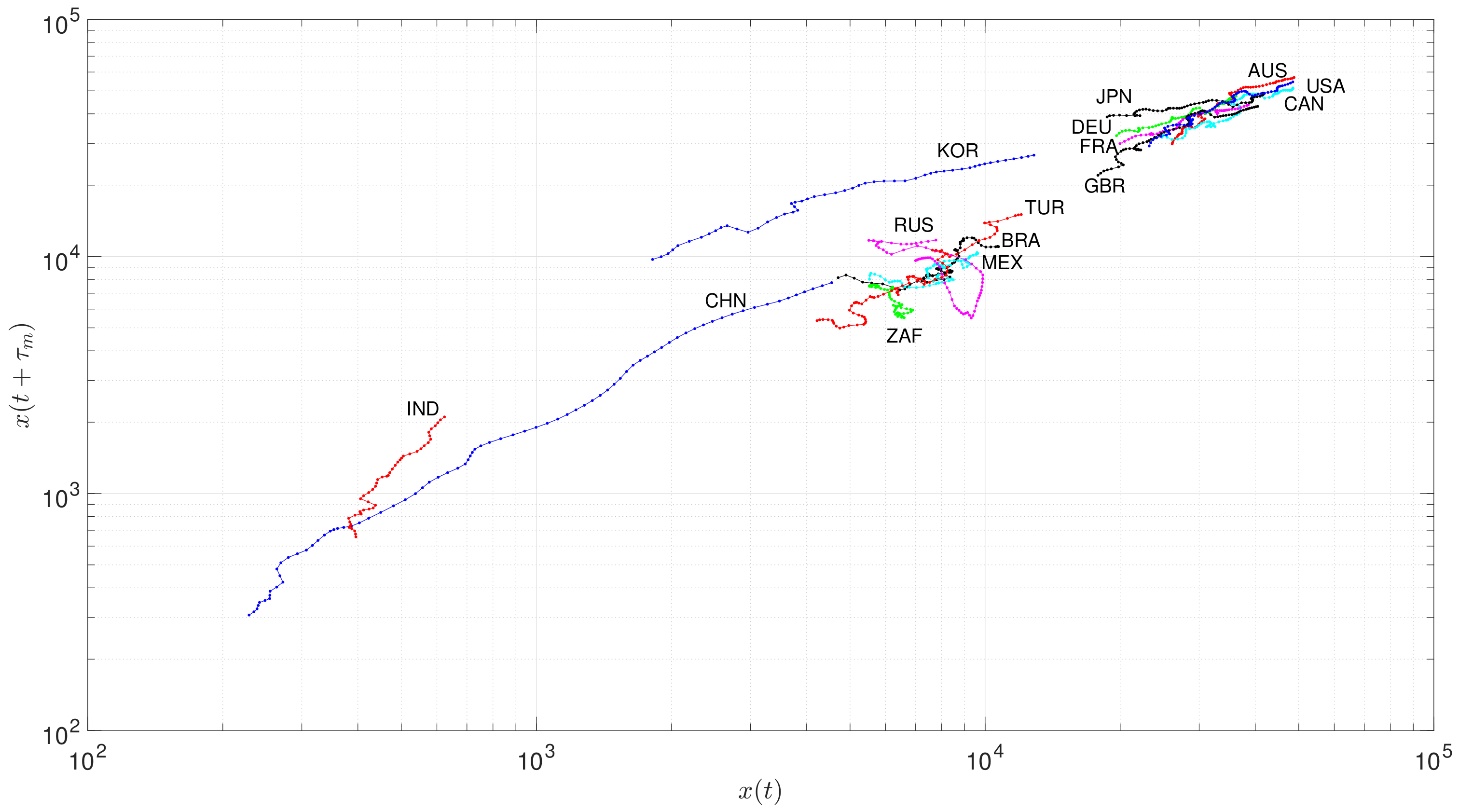
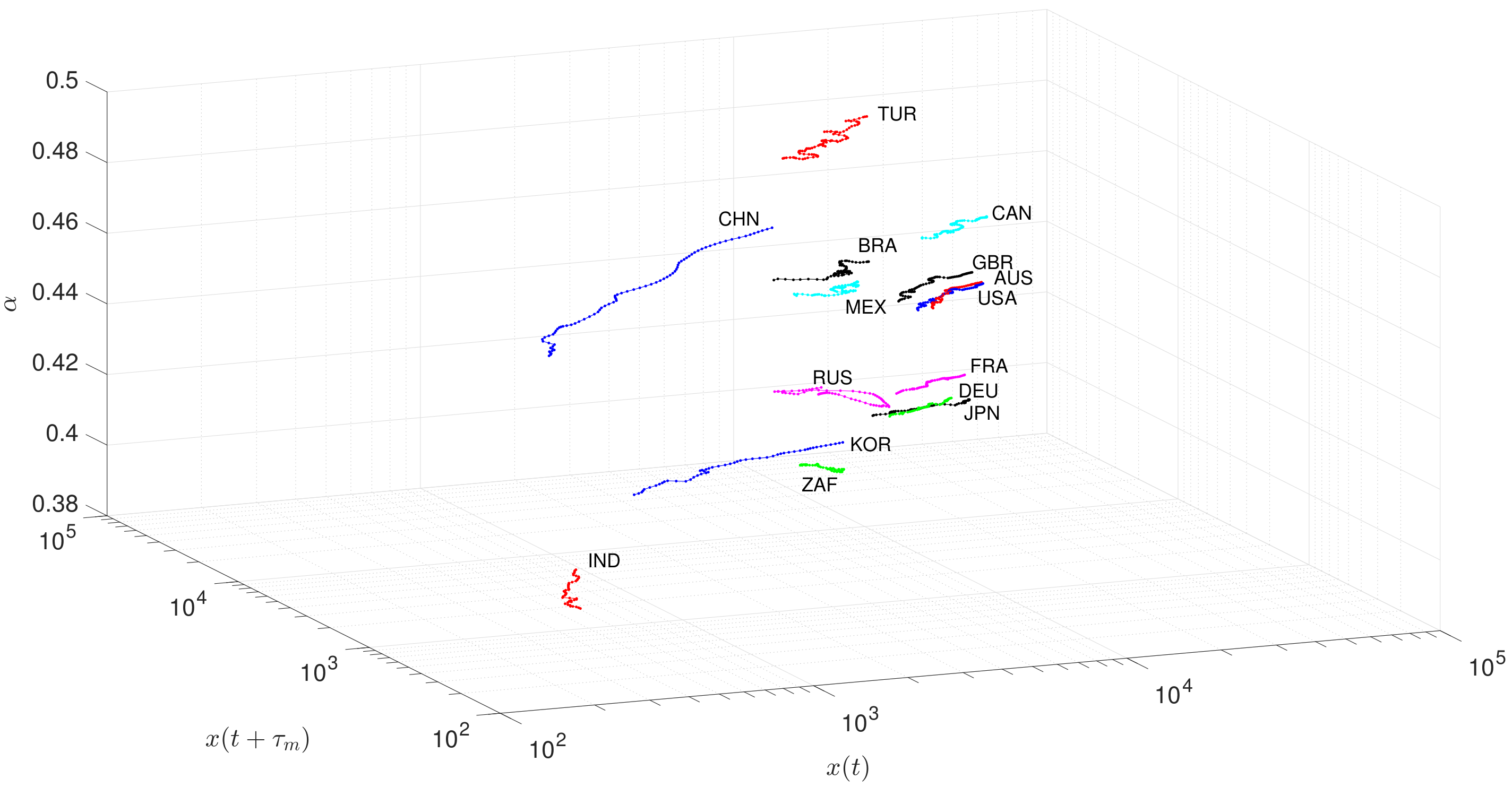
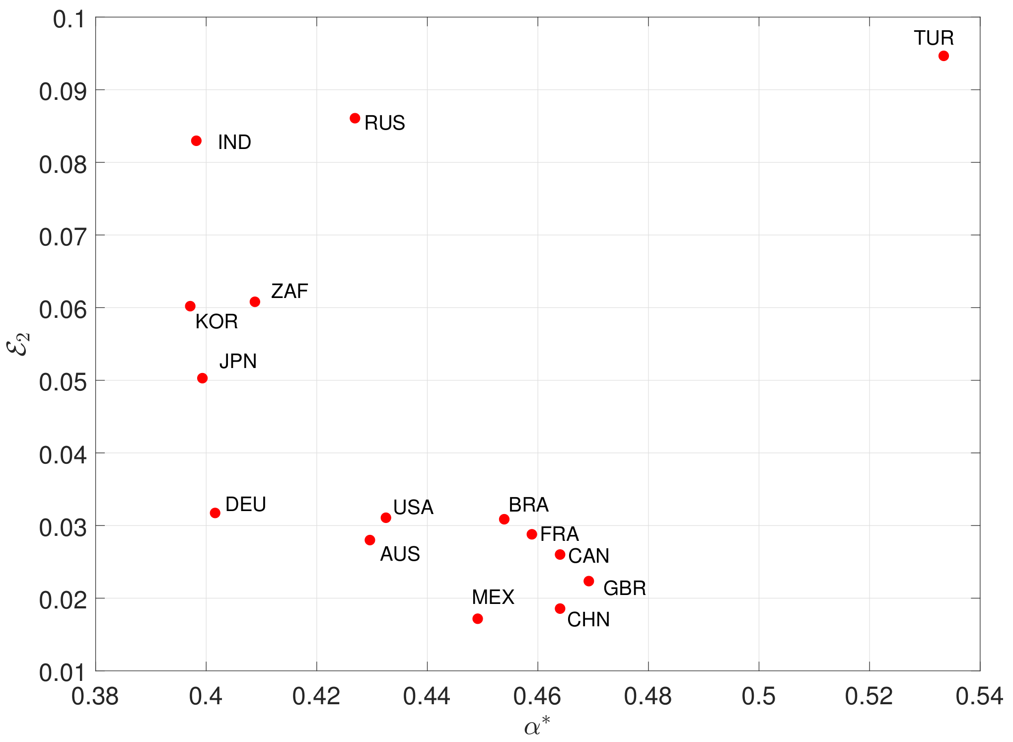
• The European partners and Japan could catch-up to the US and two other old European offshores (Australia and Canada). Before the late 1980s and the fall of the Berlin Wall, fighting communism may be considered to have been crucial to the national political strategies in most Western European countries and in East Asia. The anti-communist strategies clearly stimulated national policies in drawing them toward stock markets after the late 1980s. Many decision makers working at the World Bank and other international development agencies have even criticized codification of capital markets as meaning overregulation for the purpose of extending capitalism to communist-socialist areas.
• The heirs of old empires (Turkey and Russia), Korea, and three of the European offshores (Mexico, Brazil, and South Africa) also converged. In spite of cultural differences, genetic specificity, and climatic influences, they experimented consumption uniformization, with barriers that result from inequality in the distribution of revenue. Russia’s political change has made its transition to convergence with the most-developed economies difficult, and the country exhibits more erratic economic growth behavior, comprising periods of strong rates of growth separated by frequent and severe crises.
• The two Asian historical civilizations, China and India, have proceeded at fast and regular economic growth rates; China and India’s comparatively less-modern sectors have been catching up disproportionately faster to the world productivity frontier [44].

4. Estimation

In the last years the interest on models and algorithms for economic data forecasting has been growing [45,46]. The available methods include regression analysis [47], moving average [48], artificial neural networks [49], evolutionary computing [50], and empirical analysis [51], among others [52,53].

The proposed strategy leads implicitly to one estimation method based on the PPS. While our main objective was to establish a relationship between the time delay and the fractional order, it is relevant to explore this method and to compare results with other standard schemes.

After obtaining the value of ${\tau }_m$ for each economy and the corresponding 2-dim PPS, we have distinct alignments between the two TS, $x\left(t\right)$ and $x\left(t+{\tau }_m\right)$. This effect is negative, because it reduces the size of the intersection between the two vectors. Nonetheless, we can use the time shift between $x\left(t\right)$ and $x(t+{\tau }_m)$ for foreseeing purposes, so that the future values $\left[\widehat{x}\left(L+1\right)\cdots \widehat{x}\left(L+{\tau }_m\right)\right]$ are estimated on the basis of the old values $\left[x\left(L+1-{\tau }_m\right)\cdots x\left(L\right)\right]$. In this perspective, the new values are those that maximize the index of Equation (8) for the pair $\left[\widehat{x}\left(L+1\right)\cdots \widehat{x}\left(L+{\tau }_m\right)\right]$ and $\left[x\left(L+1-{\tau }_m\right)\cdots x\left(L\right)\right]$, as shown in the diagram of Figure 7.

The values of the delay depend on the dataset and the estimation period varies accordingly. Consequently, the estimation horizon is different for each country.

4.1. Assessing the Estimation Method

For assessing the proposed scheme we divide the available data into two subsets: 1970–2013 for prediction and 2013.5–2018 for testing. First, we calculate the delays ${\tau }_m^{*}$ for the prediction TS, since they are slightly different from the ones resulting for the complete dataset, and we predict the future values. Second, we compare the real and predicted values for the period 2013.5–2018 by means of the metrics ${\mathcal{E}}_1$ and ${\mathcal{E}}_2$, given by:

$${\displaystyle {\mathcal{E}}_1=\sqrt{\frac{1}{T}\sum _{t=1}^T{\left[x\left(t\right)-\widehat{x}\left(t\right)\right]}^2},}$$

(10)

$${\displaystyle {\mathcal{E}}_2=\frac{1}{T}\sum _{t=1}^T\frac{\left|x\left(t\right)-\widehat{x}\left(t\right)\right|}{x\left(t\right)+\widehat{x}\left(t\right)},}$$

(11)

where $T=10$ corresponds to the number of estimated points in the interval 2013.5–2018. These expressions closely follow the so-called Euclidean and Canberra distances [54] often adopted to assess the differences between numerical data.

Table 2. The values of ${\tau }_m^{*}$, ${\alpha }^{*}$, ${\mathcal{E}}_1$, and ${\mathcal{E}}_2$ for the set of 15 countries: Real data for 1970–2013 and comparison between real and estimated values for 2013.5–2018.

	AUS	BRA	CAN	CHN	FRA	DEU	IND	JPN	KOR	MEX	RUS	ZAF	TUR	GBR	USA
${\tau }_m^{*}$ (years)	13	9.5	8.5	8.5	9	19	20.5	20	21	10	13.5	17	5	8	12.5
${\alpha }^{*}$	0.430	0.454	0.464	0.464	0.459	0.402	0.398	0.399	0.397	0.449	0.427	0.409	0.534	0.469	0.433
${\mathcal{E}}_1$	3759.3	848.4	3170.7	315.3	2879.7	3278.0	325.0	6031.7	3995.9	374.3	1950.5	947.6	3764.0	2216.6	4089.5
${\mathcal{E}}_2$	0.028	0.031	0.026	0.019	0.029	0.032	0.083	0.050	0.060	0.017	0.086	0.061	0.095	0.022	0.031

includes the complete list of values $\{{\tau }_m^{*},{\alpha }^{*}\}$ of the estimation TS and the errors $\{{\mathcal{E}}_1,{\mathcal{E}}_2\}$ for all countries. Since the prediction algorithm is supported by the past, we do not obtain unrealistic values often proposed in the literature.

The errors ${\mathcal{E}}_1$ and ${\mathcal{E}}_2$ are compared with those obtained with common regression analysis. Usually, regression methods perform adequately with economic data, since the TS evolves smoothly in time [55]. We adopt the nonlinear least-squares to fit 62 distinct models to the prediction TS, while discarding those that have a large number of parameters or that depict clear divergent behavior outside the fitting interval. The best fit is obtained with the rational and the third degree polynomial functions:

$${\displaystyle {\widehat{x}}_R\left(t\right)=\frac{a+bt}{1+ct+d{t}^2},}$$

(12)

$${\displaystyle {\widehat{x}}_P\left(t\right)=a+bt+c{t}^2+d{t}^3,}$$

(13)

where $a,b,c,d\in \mathbb{R}$ are parameters to be estimated for each time series.

Equations (12) and (13) are then used for predicting the countries’ GDP per capita for the period 2013.5–2018 and for calculating ${\mathcal{E}}_1$ and ${\mathcal{E}}_2$.

Figure 8 depicts the locus of the errors obtained with the PPS method and Equations (12) and (13). We verify that the PPS method does not lead always to the best prediction. This result was expected since Equations (12) and (13) were chosen as the best between a large number of possible functions, while the PPS-based estimation is just a byproduct of the relationship between the time delay and the fractional order. Nonetheless, we must note that the PPS method yields values of ${\mathcal{E}}_1$ and ${\mathcal{E}}_2$ in the narrower interval, being more robust to the variations between the distinct country GDP per capita.

Figure 9 depicts ${\mathcal{E}}_2$ versus ${\alpha }^{*}$, revealing three clusters that comprise {IND, RUS, TUR}, {JPN, KOR, ZAF}, and {AUS, BRA, CAN, CHN, FRA, DEU, MEX, GBR, USA}, respectively. We verify the small values of ${\mathcal{E}}_2$ particularly for the third (and larger) set of countries.

4.2. Complete Estimation of GDP per Capita

We estimate GDP per capita of the set of 15 countries up to the maximum accomplished by the PPS method. This means that we have distinct prediction horizons for each country, going from 2024 for TUR up to 2042.5 for IND, as listed in

Table 3. Estimation of GDP per capita for the set of 15 countries.

	AUS	BRA	CAN	CHN	FRA	DEU	IND	JPN	KOR	MEX	RUS	ZAF	TUR	GBR	USA
$\mathit{\alpha }$	0.430	0.454	0.450	0.469	0.406	0.400	0.390	0.398	0.395	0.449	0.419	0.402	0.492	0.435	0.430
2018.5	57,908.8	11,509.6	52,625.9	8026.6	44,457.5	49,163.0	2084.8	50,188.3	27,743.1	10,273.7	10,915.1	7221.4	14,975.7	43,929.1	55,651.7
2019	58,898.2	11,992.9	53,387.6	8298.1	45,251.4	50,824.2	2065.3	51,457.0	28,724.3	9928.3	10,385.6	7002.8	15,469.5	44,872.2	56,761.7
2019.5	59,887.6	12,476.2	53,769.9	8569.7	46,045.3	52,449.0	2045.9	52,725.7	29,705.5	10,071.7	10,728.3	6784.3	15,741.7	45,815.3	57,871.6
2020	60,877.1	12,959.6	54,424.7	8841.3	46,839.2	53,163.3	2026.5	53,994.4	30,686.7	10,286.1	11,092.5	6565.7	15,993.1	46,758.4	58,981.6
2020.5	61,866.5	13,362.1	55,079.4	9112.9	47,633.1	53,701.7	2007.1	55,263.2	31,667.9	10,406.9	11,545.3	6629.8	16,368.9	47,701.5	60,091.6
2021	62,855.9	13,431.3	55,593.1	9384.5	48,427.0	53,973.0	1992.4	56,531.9	32,649.1	10,515.7	12,041.0	6710.8	16,686.6	47,397.5	61,000
2021.5	63,845.3	13,497.0	55,785.7	9656.1	49,220.9	53,947.0	2012.9	57,800.6	33,630.3	10,662.1	12,566.2	6765.2	16,809.6	47,562.3	59,875.8
2022	64,834.7	13,662.4	55,963.7	9927.7	50,014.8	53,884.5	2049.3	58,994.7	34,611.5	10,752.8	13,086.0	6824.4	16,938.8	47,831.8	58,935
2022.5	65,058.1	13,781.4	56,268.1	10,199.3	50,808.7	53,658.1	2098.5	58,961.4	35,592.7	10,754.4	13,533.4	6924.8	17,436.8	48,037.5	59,360
2023	65,271.7	13,768.1	56,665.0	10,470.9	51,602.6	53,474.2	2172.2	59,226.3	36,573.9	10,756.0	13,774.1	7049.4	17,912.0	48,238.8	59,946.1
2023.5	65,553.7	13,732.4	57,290.6	10,742.5	52,169.3	53,727.3	2243.0	59,732.2	37,555.1	10,813.4	13,233.9	7183.7	18,045.4	48,408.1	60,196.4
2024	65,956.3	13,493.9	57,706.9	11,014.1	52,749.4	54,107.9	2267.5	60,358.5	38,536.3	10,916.1	12,696.3	7330.1	18,100.0	48,595.7	60,437.7
2024.5	66,662.2	13,135.1	57,690.3	11,285.7	53,105.6	54,294.2	2288.3	61,030.6	39,517.5	11,024.9	12,907.5	7485.4		48,883.4	60,871.6
2025	67,345.2	12,795.3	57,673.7	11,557.2	53,060.8	54,523.1	2322.7	61,559.4	40,498.7	11,136.6	13,261.0	7643.9		49,262.1	61,345.8
2025.5	67,656.5	12,596.3	57,661.9	11,828.8	52,942.5	55,401.3	2357.7	62,036.6	41,479.9	11,239.3	13,544.7	7810.5		49,786.5	61,685.6
2026	67,925.5	12,608.7	57,655.0	12,100.4	52,069.1	56,601.2	2380.1	62,462.1	42,461.1	11,323.9	13,820.3	7949.7		50,333.6	62,043.4
2026.5	68,282.5	12,628.1	58,110.3		51,195.6	57,679.8	2406.4	62,881.9	43,442.3	11,378.4	14,090.5	8046.8		50,753.3	62,526.5
2027	68,639.5	12,647.4	58,672.6		51,428.2	58,527.7	2469.8	63,473.8	44,423.5	11,425.2	14,307.1	8094.7		51,104.7	63,099.1
2027.5	68,931.3	12,670.1	58,855.4		51,901.3	59,035.7	2543.5	63,847.7	45,404.7	11,473.6	14,459.3	7977.9		51,387.8	63,819.6
2028	69,239.4		58,936.1		52,441.3	59,270.6	2617.1	63,630.8	46,385.9	11,522.0	14,533.6	7860.3		51,652.7	64,441.5
2028.5	69,687.7				52,780.7	57,903.2	2690.8	63,115.6	47,367.1		14,481.8	7905.0		51,949.5	64,718.7
2029	70,106.7				52,736.0	56,535.8	2764.5	61,522.1	48,348.3		14,376.4	7982.0		52,223.6	64,977.9
2029.5	70,330.0				52,691.2	56,940.7	2838.2	59,928.6	49,329.5		14,168.9	8058.1		52,438.4	65,425.2
2030	70,550.1				52,699.9	58,474.4	2911.8	60,950.7	50,310.7		14,015.1	8119.8		52,612.4	65,993.4
2030.5	70,923.4				52,721.9	60,135.6	2985.5	62,207.9	51,291.9		14,019.7	8145.9			66,664.6
2031	71,417.3				52,817.5	61,742.2	3059.2	62,231.9	52,273.1		14,035.0	8168.8			67,461.1
2031.5					52,973.2	61,861.7	3132.8	62,250.2	53,254.3		14,114.7	8207.0
2032					53,145.6	61,932.8	3206.5	62,629.9	54,235.5		14,248.1	8238.7
2032.5					53,338.1	61,991.7	3279.4	63,284.8	55,216.7		14,394.9	8252.7
2033					53,500.4	62,068.8	3353.1	64,043.1	56,197.9		14,571.2	8258.6
2033.5					53,709.6	62,546.4	3426.8	64,640.7	57,179.1			8250.0
2034					54,259.6	63,151.6	3500.5	64,813.8	58,160.3			8230.9
2034.5					54,916.5	63,429.0	3574.1	64,969.8	59,049.7			8185.2
2035					55,383.0	63,700.3	3647.8	65,383.8	59,799.7			8149.9
2035.5					55,762.5	64,111.2	3721.5	65,832.3	60,609.0			8150.2
2036						64,601.0	3795.1	66,062.8	61,409.5			8149.6
2036.5						65,194.0	3868.8	66,310.5	62,106.2			8135.4
2037						65,750.6	3942.5	66,982.7	62,791.0			8103.3
2037.5						66,155.4	4016.2	67,700.8	63,547.0
2038						66,469.2	4089.8	68,114.8	64,341.5
2038.5							4163.5	68,374.0	65,183.4
2039							4237.2		66,028.3
2039.5							4310.8		66,813.9
2040							4384.5		67,566.9
2040.5							4458.2
2041							4531.9
2041.5							4605.5
2042							4679.2
2042.5							4752.9

. Figure 10 depicts the GDP per capita of China versus time. For this country we have ${\tau }_m=8$ years and, therefore, we have real and estimation data for the periods 1970–2018 and 2018.5–2026, respectively. Figure 11 illustrates the real and estimated PPS for all countries. Again, we verify that the PPS representation produces good evolution without abrupt changes or uncommon behavior.

5. Discussion and Conclusions

A novel approach for analyzing the dynamics of economies was developed. The method embeds the concepts of FC and PPS for processing information recorded in the TS.

From the economic history perspective it is possible to say that by 2030 the world ranking of countries’ GDPs per capita will not present significant differences from the ranking that prevails today. Australia and the US will be at the top of the ladder, followed by Canada and Japan. However, the three European countries (Germany, France, and UK), will be closer to them. Clearly, in a recovery period, optimism has prevailed in Western economies [56], but commercial warring means that some competition worries are in the air. Catching-up also expresses Western lifestyles convergence, confirming Gerschenkron [11].

Among the newly successful partners, their relative positions will change quite clearly: Today the Brazilian GDP per capita is about the same as Russia’s, much above China’s, while India remains on the tail. In the same way, distances among Brazil, Russia, and China will disappear, to make a pool of competitors. Global development of stock markets has allowed even the less-developed Russian regions to improve and ameliorate poverty [57], while the economic growth expectations in the Brazilian case will continue slowly, and growth from China relies on intensive diplomatic commercial dealings with the US [56].

Looking again to the presented forecasts, 2030 will begin a global turnover. Germany will grow and catch up to Japan. These two countries, both of which were defeated in WWII, will move ahead of France and the UK, both of which were victors in that conflict. The results from the PPS methodology indicate that India will not catch up, although it will benefit from the stimulus of strong external demand from developing economies such as China, and fast dynamics. By 2030 and even 2040 India will remain at the back, on the tail. The reason, as Battisti et al. [58] say, is that, although a country converges to its long-run growth path, such a path may be not enough and can even diverge from those countries at the global economic growth frontier. This means that for long-run performance, low levels of wealth at departure do really matter.

In a modeling perspective, exploring the combination of FC and PPS led to a new strategy for describing the dynamics of the economies while highlighting their fractional order. As a byproduct of the PPS approach, a robust algorithm for estimating the future of the TS was also obtained.

References

1. Stiglitz, J.E.; Fitoussi, J.P.; Durand, M. Measuring What Counts: The Global Movement for Well-Being; The New Press: New York, NY, USA; London, UK, 2019. [Google Scholar]
2. Stiglitz, J. It’s Time to Retire Metrics Like GDP. They Don’t Measure Everything that Matters. Available online: https://www.theguardian.com/commentisfree/2019/nov/24/metrics-gdp-economic-performance-social-progress?utm_campaign=todays_worldview&utm_medium=Email&utm_source=Newsletter&wpisrc=nl_todayworld&wpmm=1 (accessed on 26 November 2019).
3. Fogel, R.W. Capitalism and Democracy in 2040: Forecasts and Speculations; NBER Working-Paper No. 13184; National Bureau of Economic Research: Cambridge, MA, USA, 2007. [Google Scholar]
4. Bordo, M.; Eichengreen, B.; Klingebiel, D.; Martinez-Peria, M.S.; Rose, A.K. Is the Crisis Problem Growing More Severe? Econ. Policy 2001, 16, 53–82. [Google Scholar] [CrossRef] [Green Version]
5. Schularick, M.; Taylor, A.M. Credit Booms Gone Bust: Monetary Policy, Leverage Cycles and Financial Crises, 1870–2008. Am. Econ. Rev. 2012, 102, 1029–1061. [Google Scholar] [CrossRef] [Green Version]
6. Taylor, A.M. The Great Leveraging; NBER Working-Paper No. 18290; National Bureau of Economic Research: Cambridge, MA, USA, 2012. [Google Scholar]
7. Maito, E.E. The Historical Transience of Capital: The Downward Trend in the Rate of Profit Since XIX Century; MPRA Paper No. 55894; National Bureau of Economic Research: Cambridge, MA, USA, 2014. [Google Scholar]
8. Schumpeter, J.A. Business Cycles, a Theoretical, Historical and Statistical Analysys of the Capitalist Process; Martino Pub.: New York, NY, USA, 1939. [Google Scholar]
9. Hayek, F.A. The Road to Serfdom: With the Intellectuals and Socialism; Routledge: London, UK, 1944. [Google Scholar]
10. Rostow, W.W. Stages of Economic Growth, A Non-Communist Manifesto; Cambridge University Press: Cambridge, UK, 1960. [Google Scholar]
11. Gerschenkron, A. Economic Backwardness in Historical Perspective: A Book of Essays; Belknap Press of Harvard University Press: Cambridge, MA, USA, 1962. [Google Scholar]
12. Roe, M.J. Political Determinants of Corporate Governance: Political context, Corporate Impact; Oxford University Press on Demand: Oxford, UK, 2006. [Google Scholar]
13. Maddison, A. Development Centre Studies the World Economy: A Millennial Perspective; OECD Pub.: Paris, France, 2001. [Google Scholar]
14. Petráš, I.; Podlubny, I. State Space Description of National Economies: The V4 Countries. Comput. Stat. Data Anal. 2007, 52, 1223–1233. [Google Scholar] [CrossRef] [Green Version]
15. Tenreiro Machado, J.; Mata, M.E. Europe at the Crossroads of Economic Integration: Multidimensional Scaling Analysis of the Period 1970–2010. Écon. Soc. 2012, 45, 1553–1577. [Google Scholar]
16. Tenreiro Machado, J.; Mata, M.E. Multidimensional Scaling Analysis of the Dynamics of a Country Economy. Sci. World J. 2013, 2013, 594587. [Google Scholar] [CrossRef] [PubMed] [Green Version]
17. Škovránek, T.; Podlubny, I.; Petráš, I. Modeling of the National Economies in State-space: A Fractional Calculus Approach. Econ. Model. 2012, 29, 1322–1327. [Google Scholar] [CrossRef]
18. Machado, J.A.T.; Mata, M.E. A Fractional Perspective to the Bond Graph Modelling of World Economies. Nonlinear Dyn. 2014, 80, 1839–1852. [Google Scholar] [CrossRef] [Green Version]
19. Machado, J.; Mata, M.; Lopes, A. Fractional State Space Analysis of Economic Systems. Entropy 2015, 17, 5402–5421. [Google Scholar] [CrossRef] [Green Version]
20. Machado, J.T.; Mata, M.E. Pseudo-phase Plane and Fractional Calculus Modeling of Western Global Economic Downturn. Commun. Nonlinear Sci. Numer. Simul. 2015, 22, 396–406. [Google Scholar] [CrossRef] [Green Version]
21. Tarasova, V.V.; Tarasov, V.E. Logistic Map with Memory from Economic Model. Chaos Solitons Fractals 2017, 95, 84–91. [Google Scholar] [CrossRef] [Green Version]
22. Tarasov, V.E.; Tarasova, V.V. Dynamic Keynesian Model of Economic Growth with Memory and Lag. Mathematics 2019, 7, 178. [Google Scholar] [CrossRef] [Green Version]
23. Tejado, I.; Pérez, E.; Valério, D. Fractional Calculus in Economic Growth Modelling of the Group of Seven. Fract. Calc. Appl. Anal. 2019, 22, 139–157. [Google Scholar] [CrossRef]
24. Ming, H.; Wang, J.; Fečkan, M. The Application of Fractional Calculus in Chinese Economic Growth Models. Mathematics 2019, 7, 665. [Google Scholar] [CrossRef] [Green Version]
25. Skovranek, T. The Mittag-Leffler Fitting of the Phillips Curve. Mathematics 2019, 7, 589. [Google Scholar] [CrossRef] [Green Version]
26. Tarasov, V.E. On History of Mathematical Economics: Application of Fractional Calculus. Mathematics 2019, 7, 509. [Google Scholar] [CrossRef] [Green Version]
27. Samko, S.; Kilbas, A.; Marichev, O. Fractional Integrals and Derivatives: Theory and Applications; Gordon and Breach Science Publishers: Amsterdam, The Netherlands, 1993. [Google Scholar]
28. Kilbas, A.; Srivastava, H.; Trujillo, J. Theory and Applications of Fractional Differential Equations; North-Holland Mathematics Studies; Elsevier: Amsterdam, The Netherlands, 2006; Volume 204. [Google Scholar]
29. Tarasov, V. Fractional Dynamics: Applications of Fractional Calculus to Dynamics of Particles, Fields and Media; Springer: New York, NY, USA, 2010. [Google Scholar]
30. Baleanu, D.; Diethelm, K.; Scalas, E.; Trujillo, J.J. Fractional Calculus: Models and Numerical Methods; Series on Complexity, Nonlinearity and Chaos; World Scientific Publishing Company: Singapore, 2012. [Google Scholar]
31. Machado, J.T.; Lopes, A.M. Analysis of Natural and Artificial Phenomena Using Signal Processing and Fractional Calculus. Fract. Calc. Appl. Anal. 2015, 18, 459–478. [Google Scholar] [CrossRef] [Green Version]
32. Scalas, E.; Gorenflo, R.; Mainardi, F. Waiting-times and Returns in High-frequency Financial Data: An Empirical Study. Phys. A Stat. Mech. Its Appl. 2002, 314, 749–755. [Google Scholar]
33. Machado, J.T.; Lopes, A.M. Relative Fractional Dynamics of Stock Markets. Nonlinear Dyn. 2016, 86, 1613–1619. [Google Scholar] [CrossRef]
34. Lopes, A.M.; Machado, J.T.; Huffstot, J.S.; Mata, M.E. Dynamical Analysis of the Global Business-cycle Synchronization. PLoS ONE 2018, 13, e0191491. [Google Scholar] [CrossRef] [Green Version]
35. Tarasov, V.E.; Tarasova, V.V. Macroeconomic Models with Long Dynamic Memory: Fractional Calculus Approach. Appl. Math. Comput. 2018, 338, 466–486. [Google Scholar] [CrossRef]
36. Valério, D.; Trujillo, J.J.; Rivero, M.; Machado, J.T.; Baleanu, D. Fractional Calculus: A Survey of Useful Formulas. Eur. Phys. J. Spec. Top. 2013, 222, 1827–1846. [Google Scholar] [CrossRef]
37. Lopes, A.M.; Machado, J.T. Discrete-time Generalized Mean Fractional Order Controllers. IFAC-PapersOnLine 2018, 51, 43–47. [Google Scholar] [CrossRef]
38. Takens, F. Detecting Strange Attractors in Turbulence. In Dynamical Systems and Turbulence, Proceedings of a Symposium Held at the University of Warwick 1979/80; Rand, D., Young, L.S., Eds.; Lecture Notes in Mathematics; Springer: Berlin, Germany, 1981; Volume 898, pp. 366–381. [Google Scholar]
39. Ali Shah, S.A.; Aziz, W.; Nadeem, A.; Sajjad, M.; Almaraashi, M.; Shim, S.O.; Habeebullah, T.M. A Novel Phase Space Reconstruction-(PSR-) Based Predictive Algorithm to Forecast Atmospheric Particulate Matter Concentration. Sci. Program. 2019, 2019, 6780379. [Google Scholar] [CrossRef] [Green Version]
40. Holoborodko, P. Smooth Noise Robust Differentiators. 2008. Available online: http://www.holoborodko.com/pavel/numerical-methods/numerical-derivative/smooth-low-noise-differentiators/ (accessed on 26 November 2019).
41. Clark, H.; Pinkovskiy, M.; Sala-i Martin, X. China’s GDP Growth May Be Understated; Technical Report; National Bureau of Economic Research: Cambridge, MA, USA, 2017. [Google Scholar]
42. Haltmaier, J. Challenges for the Future of Chinese Economic Growth. In FRB International Finance Discussion Paper; Board of Governors of the Federal Reserve System: Washington, DC, USA, 2013. [Google Scholar]
43. Deza, M.M.; Deza, E. Encyclopedia of Distances; Springer: Berlin/Heidelberg, Germany, 2009. [Google Scholar]
44. Di Giovanni, J.; Levchenko, A.A.; Zhang, J. The Global Welfare Impact of China: Trade Integration and Technological Change; CEPR Discussion Paper; Centre for Economic Policy Research: London, UK, 2013. [Google Scholar]
45. Clements, M.P.; Hendry, D.F. Forecasting Non-Stationary Economic Time Series; MIT Press: Cambridge, MA, USA, 2000. [Google Scholar]
46. Granger, C.W.J.; Newbold, P. Forecasting Economic Time Series; Academic Press: Cambridge, MA, USA, 2014. [Google Scholar]
47. Abeysinghe, T.; Rajaguru, G. Quarterly Real GDP Estimates for China and ASEAN4 with a Forecast Evaluation. J. Forecast. 2004, 23, 431–447. [Google Scholar] [CrossRef]
48. Maity, B.; Chatterjee, B. Forecasting GDP Growth Rates of India: An Empirical Study. Int. J. Econ. Manag. Sci. 2012, 1, 52–58. [Google Scholar]
49. Kaastra, I.; Boyd, M. Designing a Neural Network for Forecasting Financial and Economic Time Series. Neurocomputing 1996, 10, 215–236. [Google Scholar] [CrossRef]
50. Claveria, O.; Monte, E.; Torra, S. Evolutionary Computation for Macroeconomic Forecasting. Comput. Econ. 2019, 53, 833–849. [Google Scholar] [CrossRef] [Green Version]
51. Gupta, M.; Minai, M.H. An Empirical Analysis of Forecast Performance of the GDP Growth in India. Glob. Bus. Rev. 2019, 20, 368–386. [Google Scholar] [CrossRef]
52. Moiseev, N.A. Forecasting Time Series of Economic Processes by Model Averaging Across Data Frames of Various Lengths. J. Stat. Comput. Simul. 2017, 87, 3111–3131. [Google Scholar] [CrossRef]
53. Bencivelli, L.; Marcellino, M.; Moretti, G. Forecasting Economic Activity by Bayesian Bridge Model Averaging. Empir. Econ. 2017, 53, 21–40. [Google Scholar] [CrossRef]
54. Deza, E.; Deza, M.M. Dictionary of Distances; Elsevier: Amsterdam, The Netherlands, 2006. [Google Scholar]
55. Xavier, S.I.M. I Just Ran Two Million Regressions. Am. Econ. Rev. 1997, 87, 178-83. [Google Scholar]
56. Stovsky, R.; Esch, K. Trendsetter Barometer: Business Outlook; Technical Report; Pricewaterhousecoopers LLP: London, UK, 2014. [Google Scholar]
57. Guriev, S.; Vakulenko, E. Breaking out of Poverty Traps: Internal Migration and Interregional Convergence in Russia; DP9675; Center for Economic Policy Research: Washington, DC, USA, 2013. [Google Scholar]
58. Battisti, M.; di Vaio, G.; Zeira, J. Global Divergence in Growth Regressions; DP 96872013; Center for Economic Policy Research: Washington, DC, USA, 2013. [Google Scholar]
Figure 1. The gross domestic product (GDP) of China, x 4 ( t ) , during 1970–2018.
Mathematics 08 00081 g001
Figure 2. The 2- and 3-dim PS of China during 1970–2018.
Mathematics 08 00081 g002
Figure 3. Locus of γ a v versus α , r and the points with maximum value γ a v = max γ a v .
Mathematics 08 00081 g003
Figure 4. The pseudo-phase space (PPS) x t x t + τ m of GDP per capita for the set of 15 countries during 1970–2018.
Mathematics 08 00081 g004
Figure 5. The locus of parameters b versus α . The markers’ size is proportional to the coefficient of determination R 2 .
Mathematics 08 00081 g005
Figure 6. The locus x t x t + τ m α of GDP per capita for the set of 15 countries during 1970–2018.
Mathematics 08 00081 g006
Figure 7. Estimation of future GDP values.
Mathematics 08 00081 g007
Figure 8. The locus of E 1 and E 2 obtained with the PPS method and Equations (12) and (13) for the set of 15 countries.
Mathematics 08 00081 g008
Figure 9. The locus of E 2 versus α * for the set of 15 countries.
Mathematics 08 00081 g009
Figure 10. The GDP per capita of China versus time: Real data for 1970–2018 and estimated values for 2018.5–2026.
Mathematics 08 00081 g010
Figure 11. The real and predicted PPS for the set of 15 countries.
Mathematics 08 00081 g011