Preference Based Portfolio for Private Investors: Discrete Choice Analysis Approach

Abstract

Behavioral finance literature shows that in addition to Markowitz’s rate of return and risk, private investors consider various other stock features. This paper discusses the problem of determining investors’ preferences for portfolio selection criteria, as well as the problem of optimal portfolio determination from the investors’ point of view. The study primarily focuses on private investors who are interested in one-time investments rather than stock trading. We use a discrete choice analysis and hierarchical Bayes method to measure individual investors’ preferences, and a logit model to determine individual shares of preferences. We treat the share of preferences as the share of certain stocks in an optimal portfolio. The proposed methodology is illustrated by the example of companies whose stocks are traded on the Belgrade Stock Exchange. We measure respondents’ preferences for companies, preferences for return rates, riskiness of stocks, and dividend rates. The results of comparing the performance of the resulting portfolio with the efficient frontier obtained using Markowitz’s portfolio theory indicate its high efficiency, thus validating the proposed approach.

1. Introduction

According to Markowitz’s [1] mean–variance portfolio theory (MVT), an optimal investment portfolio relies on the expected return and variance between assets, i.e., financial risk. To this day, it has been the dominant theory of portfolio optimization, primarily because it involves uncertainty of the portfolio return in decision making. Over time, Markowitz’s theory has been extended and improved by different approaches to modeling uncertainty. Fuzzy sets have been widely employed in portfolio optimization because the uncertainty of return can be easily quantified by fuzzy variables [2,3]. Recently, the neutrosophic theory, which extends the fuzzy concept, has been applied for solving portfolio selection problems [4] and for characterization of both portfolio performance indicators: return and risk [5]. Moreover, in the second study the authors have shown that use of neutrosophic theory enables additional information about probability of realization of the neutrosophic portfolio.

Numerous studies emphasize the importance of factors other than return, such as dividends or the firm’s financial stability [6], as having influence on portfolio decisions, especially in the case of private investors [7]. Shefrin and Statman [8] developed the behavioral portfolio theory (BPT) and showed that portfolios on the BPT efficient frontier differ from portfolios on the MVT efficient frontier. As the main reason, they suggest the fact that BPT investors, besides the expected wealth and desire for security, consider factors such as their aspiration levels and firms’ potential. In addition, according to Magron [9], BPT investors observe the portfolio differently from institutional investors. They rather perceive portfolios as pyramids of stocks, with riskless stocks that provide security at the bottom and the riskier stocks with potential for large return at the top. However, by simulating on the Center for Research in Security Prices (CRSP) database for a period of 16 years, Pfiffelmann et al. [10] have shown that 70% of the BPT optimal portfolio is located on the efficient frontier obtained by MVT.

Investors’ behavior and attitude is an open issue in portfolio theory and the number of studies that capture other important investors’ preferences beyond reward and financial risk is still limited [11]. Some behavioral finance studies have shown that investors’ behavior is influenced by various behavioral biases: overconfidence about their knowledge and skills; herding, i.e., imitating the judgments of others; home bias that means that investors prefer domestic assets, etc. [12]. In addition to behavioral factors, some social and economic factors, such as corporate reputation perceived by the investor [13], dividend taxes [14], prior experience in investment [15], or private investor’s capability of processing information [16], can also influence portfolio choice. According to [17], private investors often cannot separate their roles as investors and consumers. Consequently, such investors are not willing to invest into companies which they do not consider socially responsible (e.g., gun manufacturers).

A number of techniques examine investors behavior, and according to Strang [18], they can be classified into three groups: (1) behaviorist financial techniques, i.e., checklists, priority matrices, heuristics, etc., (2) quantitative techniques such as capital budgeting, capital asset pricing model, clustering, expected monetary value, fuzzy search, Markov analysis, and (3) multiple correspondence analysis, including methods of multidimensional scaling, simple or multiple correspondence analysis, discriminant analysis, conjoint analysis, and discrete choice analysis.

The purpose of this paper is to measure the preferences of private investors towards portfolio selection criteria and to propose an approach for determining the optimal portfolio based on those preferences. The Eckel–Grossman approach is employed to elicit investors’ attitudes to risk. Private investors’ preferences towards key portfolio choice criteria, such as return rate, risk expressed by the trend of stock prices, dividends, and perception of the company, are measured using discrete choice analysis. Portfolios based on investors’ share of preferences is compared with the optimal portfolio obtained through the traditional Markowitz’s approach, and its position relative to the MVT efficiency frontier is determined.

In this paper, we have used the method of discrete choices for several reasons. First, the choice tasks are very similar to actual buying situations in which individuals have to make trade-offs between conflicting attributes, such as risk and benefit. Second, preferences are measured indirectly, which may reduce response biases. Finally, preferences are calculated for each respondent individually and can therefore be used for post hoc segmentation purposes.

Several studies in the literature refer to the use of discrete choice analysis or other methods belonging to the class of conjoint measurement techniques for investment and portfolio decisions. According to the literature, the first attempt to empirically link behavioral phenomena to portfolio choice was made in [19]. They used the conjoint choice modeling concept to analyze investment decisions of private investors. In addition to the Markowitz framework, they examine behavioral attributes that investors may consider: home bias effect; recent events or salient characteristics; previous gains or losses; and investor’s self-assessed expertise. A total of 94 respondents were asked to distribute 1000 euros over three investment alternatives in eight different choice sets. The results of the analysis showed that both behavioral and socio-demographic factors affect portfolio choice. Bateman et al. [20] conducted a discrete choice experiment (DCE) between three options: bank account, stock, and mixed 50:50 bank account and stock, regarding two attributes: average rate of return and level of investment risk expressed as a chance of achieving a given rate. With the goal to understand the incompatibility between the type of credit offered by microfinance institutions and credit demand from agricultural households in rural Serbia, [21] conducted a choice-based conjoint with six attributes: interest rate, loan duration, loan size, grace period, euro linkage, and repayment frequency. Apostolakis et al. [22] used the choice-based conjoint analysis to examine pension beneficiaries’ preferences for a socially responsible portfolio in order to obtain valuable information for pension funds that explore investment solutions. The following attributes were included in the analysis: impact investments, socially responsible investments, and cost.

The paper is organized as follows. After the introduction part, Section 2 outlines the methodology, Section 3 describes the empirical study, while Section 4 gives the results of the study and their comparison with the results of the MVT approach. The last section presents conclusions and directions for further research.

2. Methodology

In accordance with the purpose of this study, the methods to be used in the research will first be explained. Namely, the discrete choice analysis will be used for measuring respondent preferences, while the Eckel–Grossman method will be used for measuring risk attitudes. Since the performance-based portfolio obtained through discrete choice analysis will be evaluated using MVT, Markowitz’s mean–variance model will be presented briefly.

2.1. Discrete Choice Analysis

Discrete choice analysis (DCA) is a stated preference method theoretically grounded in random utility theory (RUT) proposed by Thurstone in 1927 as a way to understand and model choices between pairs of alternatives, and Lancaster’s characteristics approach to consumer demand [23]. McFadden [24] formalized the theoretical and econometric basis of RUT needed to extend the paradigm to the general case of multiple choices and comparisons. Since then, random choice theory has been applied to a large number of cases related to human reasoning, decision making, and choice behavior, and is now the general framework for understanding and modeling different types of human behavior. Lancaster’s characteristics approach relies on the assumptions of rationality and utility maximization according to which consumers attempt to maximize their benefit derived from the product characteristics rather than from products as a whole [25,26,27].

Therefore, the DCA assumes that any product or service is defined as a combination of different levels of multiple attributes that can be both quantitative and qualitative. In the experimental procedure, individuals are presented with sets of experimentally designed alternatives that vary in the attribute levels of their component attributes, and are tasked with selecting the most preferred alternative from each choice set [28]. DCA outputs, the so-called utility scores, are numerical values that reflect the degree to which each attribute and attribute level influences individuals’ choices [29].

There are several major steps to creating a discrete choice experiment. The first step is to identify the attributes relevant to the research question and assign a level to each one. The levels should reflect the variety of possible situations that respondents can expect to experience and should be meaningful for increasing the precision of parameter estimates. An experimental design consisting of hypothetical alternatives should be further made based on attributes and levels. These alternatives are then combined into choice tasks and presented to the respondents during the survey.

Suppose that I respondents select from the set of J mutually exclusive alternatives, with each respondent receiving certain utility from each alternative. It is assumed that the individual i $(i=1,\dots ,I)$ will choose alternative j $(j=1,\dots ,J)$ if and only if the utility associated to that alternative is greater than (or equal to) the one associated with the alternative m ≠ j in the same choice set:

$$y_{ij}=\{\begin{array}{ll}1,& U_{ij}>U_{im},\forall j\ne m\\ 0,& \mathrm{otherwise}\end{array}$$

(1)

where y_ij denotes observed choice. U_ij is the utility that individual i obtains from choosing alternative j and can be decomposed into a deterministic component V_ij and stochastic component ε_ij, i.e.,

$$U_{ij}=V_{ij}+{\epsilon }_{ij}$$

(2)

Random component ε_ij represents the unobservable or unobserved sources of utility that may be due to variation in preferences among sample members and measurement error [30]. V_ij is a deterministic component of utility associated with the observed attributes that influence it. As the purpose of the choice model is to determine the degree of influence of each attribute and its levels on the utility of individuals, it is necessary to specify the functional form of this component. For this purpose, a linear additive function is usually used to map a multidimensional attribute vector to one-dimensional overall utility:

$$V_{ij}={\displaystyle \sum _{k=1}^K{\displaystyle \sum _{l=1}^{L_k}{\beta }_{ikl}{x}_{jkl}}},$$

(3)

where ${\beta }_{ikl}$ represents utility individual i attaches to level l of attribute k, $k=1,\dots ,K$, also known as part-worth utility, and $x_{jkl}$ is a binary variable that equals 1 if alternative j contains level l of attribute k, otherwise it equals 0.

Since the random component of model (2) is not observable, the respondent’s choice cannot be accurately predicted. Instead, the probability that the jth alternative is chosen by the ith respondent is determined:

$$\begin{array}{ll}{P}_{ij}(y_{ij}& =1)=P(U_{ij}\ge U_{im}|m\in J,\forall m\ne j)\\ & =P(V_{ij}+{\epsilon }_{ij}\ge V_{im}+{\epsilon }_{im}|m\in J,\forall m\ne j)\\ & =P({\epsilon }_{ij}-{\epsilon }_{im}\ge V_{im}-V_{ij}|m\in J,\forall m\ne j)\\ & =P({\epsilon }_{im}\le V_{im}-V_{ij}+{\epsilon }_{ij}|m\in J,\forall m\ne j)\end{array}$$

(4)

Expression (4) is estimated depending on the assumptions about the distribution of random components.

Multinomial logit (MNL) model or Hierarchical Bayes (HB) estimation can be used to estimate model parameters i.e., part-worth utilities associated with attribute levels. The MNL model (McFadden, 1974) is based on the assumption that random components ${\epsilon }_{ij}$ have the same probability distribution and that all are mutually independent (the so-called i.i.d. property), with the Weibull density function and the variance of the error equal to ${\pi }^2/6$.

The multinomial logit model of choice assumes that the probability of choosing any alternative is proportional to the exponent of its deterministic utility value [31]:

$$P_{ij}(y_{ij}=1)=\frac{\exp (V_{ij})}{{\displaystyle \sum _{m\in J}^{}\exp (V_{im})}}=\frac{1}{1+{\displaystyle \sum _{m\in J}^{}\exp (V_{im}-V_{ij})}}$$

(5)

The parameters in the multinomial logit model do not vary depending on the choices, therefore the vector of part-worths (β) is estimated at aggregate level, i.e., for the overall sample, by maximizing the logarithmic likelihood function given by the following expression:

$$\ln (L(\beta ))={\displaystyle \sum _{i=1}^n{\displaystyle \sum _{j=1}^J{y}_{ij}\cdot \ln P_{ij}}}$$

(6)

However, this study used the HB approach due to its ability to estimate individual-level parameters. HB estimation implies that hierarchical models are analyzed using Bayesian methods where probability is expressed as a degree of belief. In the HB approach, respondents are seen as members of a heterogeneous sample, and it is assumed that the estimated parameters (part-worths) have the multivariate normal distribution described by the mean vector and the covariance matrix. Initially, prior beliefs (distributions) are assigned for the parameters which are then updated using Bayesian theorem. The probability that a respondent will choose a particular alternative is calculated on the basis of the expression (5), while the individual part-worths are estimated using Monte Carlo simulation techniques. An advantage of the HB model lies in its ability to estimate more parameters with fewer data collected from each respondent.

The estimated part-worth $\widehat{\beta }$ of a level reflects how strongly that level influences the decision to choose a particular alternative. Attributes with large variations of part-worths are considered more important. Accordingly, the relative importance of each attribute for each respondent is calculated by dividing the utility range for a given attribute by the sum of the utility ranges for all attributes [32]:

$$R{I}_{ik}=\frac{\underset{l}{\max }{\widehat{\beta }}_{ikl}-\underset{l}{\min }{\widehat{\beta }}_{ikl}}{{\displaystyle \sum _{k=1}^K\left(\underset{l}{\max }{\widehat{\beta }}_{ikl}-\underset{l}{\min }{\widehat{\beta }}_{ikl}\right)}},i=1,\dots ,I,k=1,\dots ,K.$$

(7)

These individual values of the relative importance of attributes can be used further to calculate the attributes importance for the sample as a whole if the preferences prove to be homogeneous, or at the cluster level in the case of heterogeneous preferences. Part-worths can also be used to predict the share of preferences for different options in competitive scenarios. A variety of models can be used for simulation purposes. The first-choice model assumes that each respondent can choose only one alternative, the one that maximizes utility, while the share of preference model, also called logit simulation, allows respondents to choose options in a probabilistic manner.

Let ${\widehat{\beta }}_{kl}$ be parameters estimated by the HB method, i.e., part-worths for each level of each attribute. If a total of S different alternatives are considered, then the share of preferences (P_s) for the alternative s can be calculated by:

$$P_s=\frac{\exp \left(b{\displaystyle \sum _{k=1}^K{\displaystyle \sum _{l=1}^{L_k}{\widehat{\beta }}_{kl}{x}_{jkl}}}\right)}{{\displaystyle \sum _{j=1}^S\exp \left(b{\displaystyle \sum _{k=1}^K{\displaystyle \sum _{l=1}^{L_k}{\widehat{\beta }}_{kl}{x}_{jkl}}}\right)}},s\in S.$$

(8)

The scale parameter b is used to fine-tune the results so that they reflect the respondents’ behavior more accurately. Namely, this parameter is used to reflect the variance of the unobserved portion of utility, i.e., unobserved preference uncertainty [33]. Researchers claim that some individuals act more randomly in choice situations than others, leading to a “scale heterogeneity” [34]. According to Fiebig et al. [34], scale heterogeneity increases with task complexity, especially when those tasks involve decisions about risks and probabilities.

2.2. The Eckel–Grossman Method

Several experimental procedures have been developed to measure individuals’ risk preferences. Eckel and Grossman [35] developed a method for eliciting risk preferences that produces enough heterogeneity in choices to allow for the estimation of utility parameters [36]. The advantage of this measure is its simplicity, focusing on expected returns and variance.

In the Eckel–Grossman method, individuals are offered a set of gambles and are asked to choose the one that they would like to play. Eckel and Grossman originally proposed the five-gamble version, while Dave et al. [37] adapted it to include a set of six gambles (see

Table 1. The Eckel–Grossman gamble choices.

Choice (50/50 Gamble)	Low Payoff	High Payoff	Expected Return	Standard Deviation	CRRA Range
Gamble 1	28	28	28	0	3.46 < r
Gamble 2	24	36	30	6	1.16 < r < 3.46
Gamble 3	20	44	32	12	0.71 < r < 1.16
Gamble 4	16	52	34	18	0.50 < r < 0.71
Gamble 5	12	60	36	24	0 < r < 0.50
Gamble 6	2	70	36	34	r < 0

Source: [36].

). Choosing each of the gambles in the choice set gives a 50% chance of getting a low payoff and a 50% chance of making a high payoff. The gambles increase in both expected return and risk (standard deviation of the expected payoff) moving from Gamble 1 to 6. The set of gambles contains a risk-free alternative (Gamble 1) that includes a guaranteed payout of 28 with a variance equal to zero. Moving from Gamble 1 to Gamble 5, there is an increase in both expected return and risk (standard deviation), with expected return increasing linearly with standard deviation. Gamble 6 expected return is the same as for Gamble 5, but the standard deviation is much higher, indicating a high-risk alternative.

The gambles are designed so that risk-averse individuals would choose lower risk gambles, i.e., gambles with both lower standard deviation and lower returns (Gambles 1–Gambles 4). Individuals who are risk-neutral would choose Gamble 5 which has the highest return rate, while Gamble 6 would be selected only by risk-seeking individuals.

For all possible Gambles, ranges of the relative risk aversion coefficients, assuming constant relative risk aversion (CRRA), are given in Table 1. The ranges are determined by comparing gambles with its neighbors and calculating a value of r that generates the same level of utility for the payoffs associated with each neighboring gamble. Based on this measure, individuals who choose gamble with r > 0 can be classified as risk averse, those who choose gamble with r < 0 as risk seeking, while choosing an option with r = 0 categorizes the individual as risk neutral.

2.3. Mean–Variance Portfolio Optimization

Markowitz’s mean–variance theory refers to the trade-off between two conflicted criteria for portfolio selection: risk and return. The expected return is calculated as a mean of return rates, which should be maximized, while the portfolio risk is measured as the covariance of return rates and it should be minimized.

Let us consider n stocks and their prices p_i in the observed period T, i = 1, ..., n. Based on the prices, the return rate r_it can be calculated as $r_{it}=(p_{it}-p_{it-1})/p_{it-1}$ for each stock i in each period t, t = 1, ..., T. The goal is to determine an optimal investment proportion vector $w=(w_1,w_2,\dots ,w_n)$, also called a portfolio, thus maximizing the total expected return of investment. Variable $w_i,i=1,\dots ,n$ represents the proportions of the initial sum to be invested in stock i [38]. Therefore, ${\displaystyle {\sum }_{i=1}^n{w}_i}=1$. Let $\mu =({\mu }_1,{\mu }_2,\dots ,{\mu }_n)$ be the vector of the expected returns of the n stocks, where each ${\mu }_i$ is calculated as ${\mu }_i={\displaystyle {\sum }_{t=1}^T{r}_{it}}/T$. Then, the expected portfolio return can be expressed as: $E[w]={\displaystyle {\sum }_{i=1}^n{\mu }_i\cdot w_i}$. The risk of the portfolio is then defined using covariance matrix $\mathsf{\Sigma }=({\sigma }_{ij})$ where ${\sigma }_{ij}$ denotes the covariance for the stocks i and j. Then, the risk of the portfolio can be expressed as: $Cov[w]={\displaystyle {\sum }_{i=1}^n{\displaystyle {\sum }_{j=1}^n{w}_i{\sigma }_{ij}{w}_j}}$. The problem of portfolio optimization can be formulated in two ways: maximize the expected portfolio return for a given risk level $\sigma$ or minimize portfolio risk for a given expected return r.

The formulation of the mathematical model for portfolio optimization (MMOP) is as follows:

$$\begin{array}{cc}\begin{array}{l}\max {\displaystyle \sum _{i=1}^n{\mu }_i{w}_i}\\ \mathrm{s}.\mathrm{t}.\\ {\displaystyle \sum _{i=1}^n{\displaystyle \sum _{j=1}^n{w}_i}{\sigma }_{ij}{w}_j}\le \sigma \\ {\displaystyle \sum _{i=1}^n{w}_i}=1\\ w_i\ge 0,i=1,\dots ,n\end{array}& \end{array}$$

(9)

By incrementally increasing the value of the parameter $\sigma$, the mean–variance efficiency frontier and the diversification of actions are obtained. Based on them, the investor makes the final decision on an acceptable portfolio.

3. Study Design

The experiment was conducted using an online survey administered through the Conjoint.ly platform and it contained four sections: (1) respondents’ knowledge and experience regarding stock trading; (2) discrete choice tasks; (3) gamble choice game; and (4) socio-demographic questions (see Supplementary Materials).

The first section contained two self-assessment items:

• Knowledge of financial investments that was evaluated on a 5-point Likert scale, where 1 implies absolute unfamiliarity and 5 implies that the respondent is very familiar with the topic;
• Experience in stock trading with the choices offered: Yes, I have personally traded; Yes, I used service brokers; No.

In order to elicit respondents’ preferences using DCE, four key attributes were selected based on literature review, expert opinions, and stock market analysis. The list of selected attributes and their levels are given in

Table 2. Attributes and their levels covered by the study.

Attribute	Attribute Levels
Company	Metalac a.d.
	Nikola Tesla Airport
	Jedinstvo a.d.
	Energoprojekt holding
Return rate	0%
	0.05%
	0.10%
	0.15%
Dividend (% of money invested)	0%
	1.5%
	3.0%
	4.5%
	6%
The trend of the stock prices over the past 3 years (graphics)	Trend 1
	Trend 2
	Trend 3

Source: Authors.

.

The Company attribute is included in the study primarily to determine the extent to which the perceptions of a particular company and the company’s industry affect the respondents’ preferences. Four companies known to the majority of citizens of the Republic of Serbia are defined as levels for this attribute: Metalac a.d., Nikola Tesla Airport, Jedinstvo a.d., and Energoprojekt holding. These companies are on the Prime and Standard Listings on the Belgrade Stock Exchange [39].

The second attribute in this study is the return rate in the previous year. It indicates the success of a company’s business and can be significant when considering to sell the shares after a certain period of time. Attribute levels represent the values (percent) within the range of market values.

The third attribute—dividend—provides information on the portion of the company’s profit that would be paid to shareholders at the end of the accounting period. It can be very important to the respondents since it shows which part of the company’s profit will be distributed among the shareholders. As the study focuses on private investors interested in one-time investment rather than stock trading, the amount of dividend is an important factor in their choice. The attribute levels are expressed as percent from 0% to 6%.

The last attribute (trend) refers to the changes of the stock price over the past three years. This attribute is significant for the final results of the study because it refers to the long-term quality and stability of the company’s business. The levels for this attribute are defined through a graphic representation of certain trends (Table 2). Based on the trends shown on the graphics in the survey, respondents can conclude on the risk of investment, as well as on potential profits that can be realized by investing in one of the offered stocks, which can certainly have an impact on their final choice.

The Conjoint.ly online platform was used to create an efficient experimental design. A total of three different blocks of 10 tasks with three alternatives (investment options) were generated. In each choice task, respondents also had the option to deposit money with the bank at an interest rate of 0.5% per annum. The respondents chose this option if they felt that none of the stock investing options was appropriate for them.

There are a number of techniques to calculate the sample size for discrete choice experiments, but they are all influenced by the dimension of the experimental design generated [40]. According to Orme [41], the rule of thumb for an acceptable sample size is given by I × t × a/c ≥ 500, where I represents the minimum sample size, i.e., the required number of respondents, t is the number of choice tasks presented to each respondent, a is the number of alternatives in each choice task, and c represents the highest number of levels within all attributes individually. Applying Orme’s rule, the minimum acceptable sample size for this study was 84 (I ≥ 500 × 5/(10 × 3) ≈ 84).

At the very beginning of the survey, participants were given a set of instructions. As the aim of the research was to understand and explain participants’ investment choices in hypothetical circumstances, we asked them to imagine that they had 100,000 euros available to invest either in stocks or to deposit into a bank. Participants were then informed that the investment options differ in four attributes and attribute levels. Given the rather specific research topic, each of the attributes and corresponding levels were briefly explained. Afterwards, participants were instructed that the investment options could differ in four attributes, which were then presented together with their respective levels.

In order to provide a more detailed insight into the sample characteristics and an adequate analysis of the results, some additional questions were posed to the respondents. In addition to the introductory questions related to the financial knowledge and experience of the respondents and the discrete choice tasks, the questionnaire included another set of questions related to the socio-demographic characteristics of the respondents, as well as their attitude towards risk. Socio-demographic characteristics have been examined through questions regarding gender, age, level of education, employment status, and marital status. In order to measure attitude towards risk, respondents were first asked about their willingness to take risk in financial investments (on the 5-point Likert scale), and were then tasked to choose the gamble option in the Eckel–Grossman six-gamble game.

4. Survey Results

Survey data were collected in October 2017 through the Conjoint.ly platform. A total of 624 individuals joined the survey, but only 194 completed it fully (31.1% response rate). The responses of 25 individuals (12.9%) were excluded from the analysis due to poor quality caused by randomly picked responses, short completion time, or inconsistencies. The average time taken to complete the questionnaire was approximately 9 min. In sum, the number of valid questionnaires used in the analysis was 169. Since each respondent was presented with 10 choice tasks with three alternatives (investment options), a total of 1690 choices were available for analysis.

4.1. Sample Characteristics

Almost two-thirds of the sample were female respondents (63.31%). The average age of the respondents was 29.52 years (S.D. = 9.51), with the youngest respondent being 18 years old and the oldest being 63 years old. The majority of the sample consisted of respondents who were single in terms of marital status (58.58%), holding a university degree (87.57%), and those working full-time (56.8%). Detailed demographics are given in

Table 3. Demographic data.

Demographic	Category	Percent
Gender	Male	36.69%
	Female	63.31%
Marital status	Single	58.58%
	Married without kids	5.92%
	Married with kids	18.93%
	Other	16.57%
Highest level of completed education	High school	7.69%
	Undergraduate/graduate study	87.57%
	PhD	3.55%
	Other	1.18%
Employment status	Unemployed	21.30%
	Internship/part-time job	13.61%
	Full-time job	56.80%
	Retired	1.18%
	Other	7.10%

Source: Authors calculations.

.

4.2. Respondents’ Preference towards Financial Investments and Risk

Asked to evaluate their awareness about the topic of financial investments on a scale from 1 to 5, respondents assessed their knowledge with an average score of 2.5, indicating a moderate level of knowledge. On the other hand, as for the trading in stocks, the vast majority of the respondents stated that they do not have such experience (91.72%). Only 5.33% of the respondents used broker services in stock trading, while 2.96% of them personally traded on the stock exchange.

When it comes to taking investment risks, an average score of 2.7 on the self-assessment task suggests a neutrality to risk (for the female population the score is 2.55, while for the male population it is 3.06). Therefore it can be concluded that female respondents consider themselves more risk averse, which is in line with the Eckel and Grossman [35] findings. The results of Eckel–Grossman method in our study shows that only 4.14% of the respondents are risk-seeking, 11.83% are neutral, while the remainder (84.03%) have a risk aversion (see

Table 4. Distribution in the Eckel–Grossman gamble game.

Choice (50/50 Gamble)	Low/High Payoff	Risk Attitude	Female	Male	Sample
Gamble 1	28/28	Extremely risk averse	9.35%	11.29%	10.06%
Gamble 2	24/36	Risk averse	27.1%	25.81%	26.63%
Gamble 3	20/44	Risk averse	38.32%	27.42%	34.32%
Gamble 4	16/52	Risk averse	9.35%	19.35%	13.02%
Gamble 5	12/60	Risk neutral	12.15%	11.29%	11.83%
Gamble 6	2/70	Risk seeking	3.74%	4.84%	4.14%

Source: Authors calculations.

). In terms of gender, these results are not consistent with previous ones. Specifically, it can be observed that a higher percent of male than female respondents exhibit extreme risk aversion but also risk seeking.

4.3. Aggregated Preferences towards Portfolio Selection Criteria

Using the HB method, the utility parameters for each respondent in the sample were assessed, as well as for the sample as a whole.

Table 5. Relative utility and importance scores.

Attribute	Level	Relative Utility Score (Part-Worths)	Relative Importance Score (Attributes Importance)
Company	Metalac a.d.	3.35	9.49%
	Nikola Tesla Airport	3.00
	Jedin a.d.	−6.14
	Energoprojekt holding	−0.21
Return rate	0%	−4.13	8.93%
	0.05%	−1.57
	0.1%	0.90
	0.15%	4.80
Dividend	0%	−28.14	48.98%
	1.5%	−6.57
	3%	1.57
	4.5%	12.30
	6%	20.84
Trend	Trend 1 (non-risky)	12.25	32.6%
	Trend 2 (moderate risky)	8.10
	Trend 3 (risky)	−20.35

Source: Authors calculations.

shows the average part-worth utilities for each level of each attribute and the importance scores for each of the attributes calculated using Equation (7). Part-worths explain the contribution of the levels of each attributes to the overall utility, allowing one to understand how changing the level affects investors’ preferences for a particular investment option. Higher part-worth utility values indicate greater preference.

As can be seen from Table 5, the dividend was found to have the most significant influence on respondents’ preferences with a relative importance of 48.98%. The trend of stock prices in the previous three years is the second most important attribute which on average receives 32.6% of preferences, while the importance of the other two attributes is by far lower. Namely, company and return rate were observed as the least-valued attributes (9.49% and 8.93% respectively).

The part-worth utilities of each attribute are scaled so that their sum is always zero and should be considered as relative values. Looking at the most important attributes (dividend), respondents prefer the highest offered level (utility of 20.84), as was expected. On the other hand, the level that implies that investors do not participate in the profit distribution (dividend is 0%) has a negative partial utility (−28.14). The positive value of utility also has levels of 3% and 4.5%, while the dividend amount of 1.5% is negatively perceived by respondents.

Risk aversion of the sample can be seen clearly through preferences associated to the levels of the trend attribute. Results show that respondents have a markedly negative perception of the risk-taking trend (trend 3), while they show strong preferences towards a moderate, and especially non-risky, trend.

When it comes to the attribute company, it is clear that respondents prefer Metalac a.d. most, followed by Nikola Tesla Airport, while Jedinstvo a.d. is unattractive for respondents with negative part-worth value. As with the dividend attribute, the signs of the part-worths of the return rate attribute were also in line with a priori expectations. Specifically, respondents showed the least preference for a return rate of 0%, and their preferences increased as the rate of return increased.

Analysis of the 20 most desirable options indicates that in 18 out of 20 options the dividend value is equal to 6%, which is also the most important stocks feature for the respondents. Also, the option relating to the shares of Jedinstvo a.d. appears for the first time on the 18th place on the list, an option that includes a 0% return rate on 16th, while only low and moderate risk trends occur in the top 20 options.

We further investigated whether risk attitudes according to the Eckel–Grossman method correlate with respondents’ preferences when it comes to stock riskiness (expressed via trend attribute). Although some correlations were found they are not statistically significant (see

Table 6. Correlations between respondents’ risk attitudes according to the Eckel–Grossman method and preferences towards levels of trend attribute (stock riskiness).

Risk Attitude		Trend 1	Trend 2	Trend 3
Extremely risk averse (Gamble 1)	Part-worths	13.36	8.51	−21.86
	Pearson Correlation	0.072	0.056	−0.087
	Sig. (2-tailed)	0.354	0.473	0.258
Risk averse (Gamble 2)	Part-worths	13.13	8.67	−21.80
	Pearson Correlation	0.000	0.038	−0.020
	Sig. (2-tailed)	0.998	0.626	0.796
Risk averse (Gamble 3)	Part-worths	12.12	8.73	−20.85
	Pearson Correlation	0.029	0.083	−0.078
	Sig. (2-tailed)	0.705	0.285	0.315
Risk averse (Gamble 4)	Part-worths	10.54	5.68	−16.21
	Pearson Correlation	−0.080	−0.158 *	0.164 *
	Sig. (2-tailed)	0.298	0.041	0.033
Risk neutral (Gamble 5)	Part-worths	11.66	6.26	−17.92
	Pearson Correlation	−0.008	−0.096	0.059
	Sig. (2-tailed)	0.922	0.216	0.444
Risk seeking (Gamble 6)	Part-worths	9.80	8.31	−18.11
	Pearson Correlation	−0.030	0.057	−0.011
	Sig. (2-tailed)	0.702	0.464	0.883

* Correlation is significant at the 0.05 level (2-tailed). Source: Authors calculations.

). For example, respondents who are extremely risk-averse have the lowest preferences for Trend 3 and the highest for Trend 1 compared to all types of respondents.

4.4. Preference Based Segmentation

A detailed analysis of the respondents’ part-worth utilities indicated great heterogeneity of their preferences. For that reason, k-means cluster analysis of individual utilities was performed to classify respondents into homogeneous groups of similar preferences. As a result, four segments were identified: inexperienced segment (19% of total sample), mainstream segment (43%), trend oriented segment (18%), and brand-oriented segment (20%). 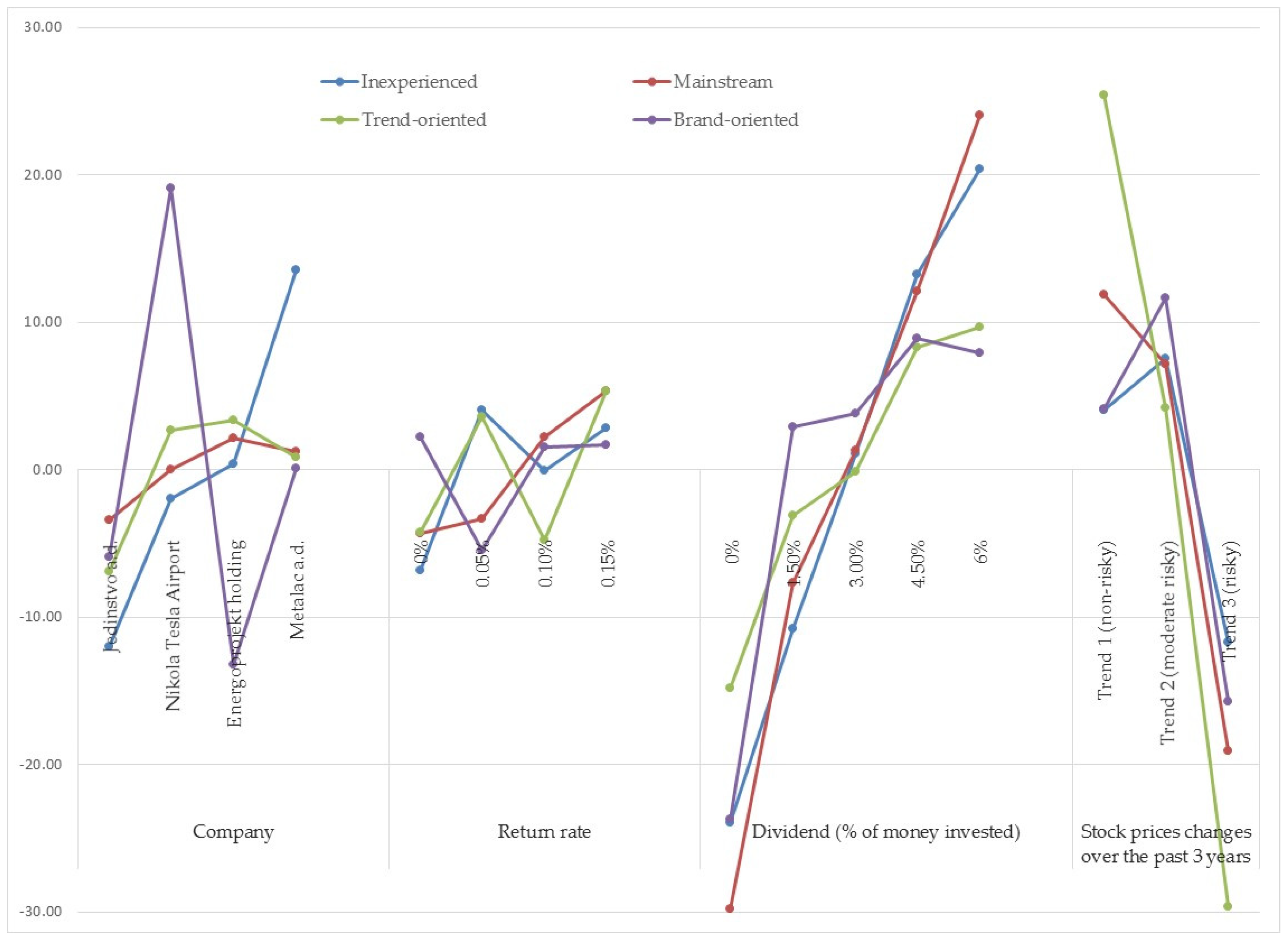Relative importance of attributes for those segments are shown in Figure 1. As demonstrated, the dividend is the most important attribute for as many as three out of four segments.

Similarly, members of the brand-oriented segment barely take into account the return rate of stocks, assigning almost equal importance to other attributes. This segment is highly specific and implies significant deviations from the rest of the sample when it comes to the company attribute. Namely, respondents strongly prefer Nikola Tesla Airport, they are indifferent to the company Metalac a.d., while the other two companies are extremely unpopular. This segment is specific for its greater proportion of the female population when compared to other segments, as well as being the youngest.

Within the mainstream segment, in addition to the dividend, the trend attribute is also of great importance, while the remaining two attributes are negligibly important. The name mainstream is based on the fact that their preferences largely match the average preferences of the entire sample. Members of this segment have more experience in financial investments, most of them are full-time employees and more willing to take risks when making investment decisions. When it comes to company attribute, they express preferences for Energoprojekt holding and Metalac a.d. (Figure 2).

A segment of inexperienced, in addition to dividend, bases its choices on the company attribute (preferring Metalac a.d.) and somewhat on the trend attribute (preferring Trend 2), and considers the rate of return relatively unimportant. The main feature of this segment is that none of its members ever personally traded stocks.

The trend-oriented segment, the smallest one with 18% share, is the only segment in which the dividends attribute has no major influence on decision making. Namely, respondents belonging to this segment made decisions primarily on the basis of the changes of the stock price over the past three years (significance of up to 55%). On the other hand, attributes related to the company and the return rate have no particular importance. Nevertheless, the members of this segment prefer Nikola Tesla Airport and Energoprojekt holding, while the negative value of utility was realized only by the company Jedinstvo a.d. Knowledge of financial investments in this segment is lower than in other segments and is 2.3 out of 5.

Examining whether members of different clusters have different risk preferences according to the Eckel–Grossman method, it was found that there is no statistically significant difference between clusters.

4.5. Portfolio Based on Investors’ Share of Preferences

Logit model was used to predict optimal portfolio from the perspective of private investors. Averaged respondents’ shares of preferences are observed (treated) as shares of stocks in portfolio. Firstly, the actual values of stock market indicators for the companies covered by the study were determined. Then, each of these values was associated with the closest level of the corresponding attribute in the discrete choice analysis (

Table 7. Actual indicators’ values and corresponding attribute levels from DCE.

Company	Return Rate		Dividends		Trends
	Actual	Attribute Level	Actual	Attribute Level	Actual
Nikola Tesla Airport	0.12%	0.1%	4.54%	4.5%	Trend 2
Metalac a.d.	0.01%	0%	8.35%	6%	Trend 1
Energoprojekt holding	0.09%	0.1%	1.28%	1.5%	Trend 3
Jedinstvo a.d.	0.02%	0%	4.24%	4.5%	Trend 1

Source: BELEX [39] and authors.

).

By varying the value of the scale parameter b, share of preference was simulated using Equation (8), for both the sample as a whole and for each segment separately. As mentioned in Section 2.1, the scale parameter is a measure of the importance of the deterministic part of a random utility model relative to the idiosyncratic part. Czajkowski et al. [42] found that as the experience of individuals increases, the value of the scale parameter increases while the heterogeneity of the scale decreases.

Given that the research sample lacked experience in stock trading, simulations were also performed for lower values of the scale parameter b than the default value of 1. The results of the simulations for the sample as a whole are shown in

Table 8. Whole-sample preferences based portfolios for different values of scale parameters.

	Scale Parameter	Nikola Tesla Airport	Metalac a.d.	Energoprojekt Holding	Jedinstvo a.d.
Portfolio 1	b = 1	29.68%	56.59%	0.50%	13.23%
Portfolio 2	b = 0.9	30.33%	54.23%	0.77%	14.66%
Portfolio 3	b = 0.8	30.88%	51.76%	1.18%	16.18%
Portfolio 4	b = 0.7	31.28%	49.15%	1.80%	17.77%

Source: Authors calculations.

.

It is clearly observable that for all values of parameter b, the company Metalac a.d. achieves at least 50% of the preference share in simulated portfolios. The main reason for such a positioning lies predominantly in the value of the dividend, as the most important attribute, but also in the values of attributes trend and company that achieve positive part-worths (see Table 5). On the other hand, negligible share of Energoprojekt holding’s stocks in all four simulated portfolios can be explained by the low values of the company’s indicators, and by poor perception of the company by the respondents.

Figure 3 shows the portfolios across the four segments for different values of scale parameter b. As for the entire sample, in all four segments the share of Energoprojekt holding’s stocks in the portfolio is negligible regardless of the value of parameter b. In the first three clusters, Metalac a.d. has the largest share of stocks in all simulated portfolios, but this percentage decreases slightly with the decrease in scale parameter b, while the share of the remaining three companies increases with the decrease of b. The fourth cluster differs significantly from the remaining three clusters in that the optimal portfolio is dominated by the shares of Nikola Tesla Airport stocks, but with the decrease in value of b, the percentage decreases while the share of the other three companies increase.

5. Optimization and Simulation Results

In this paper, we investigate private investors’ preferences rather than the preferences of stock brokers or institutional investors. Respondents of the survey decide according to return rate and dividend, so the objective of the mathematical model (9) is extended by dividend according to [43].

The daily return rates for the period between 30 June 2016 to 30 June 2017 for companies Metalac a.d., Nikola Tesla Airport, Jedinstvo a.d., and Energoprojekt holding were collected from [40]. The expected returns and dividends $({\mu }_i)$, standard deviations, and correlations of the stocks are given in

Table 9. Stocks data of the selected companies.

	Nikola Tesla Airport	Metalac a.d.	Energoprojekt Holding	Jedinstvo a.d.
Return rate	0.12	0.01	0.09	0.02
Dividend	4.54	8.35	1.28	4.24
Standard deviation	1.65	1.36	1.71	1.87
Correlation
Nikola Tesla Airport	1
Metalac a.d.	−0.0291	1
Energoprojekt holding	−0.0703	−0.0539	1
Jedinstvo a.d.	0.0857	0.0095	−0.0067	1

Source: Authors calculations.

.

First, for each portfolio (scale parameter) from Table 8, the total expected return and risk $(\sigma )$ were calculated as explained in Section 2.3. Then, the MMOP was solved for calculated values of $\sigma$. The risk, preference-based expected return (PBR), optimization-based expected return (OBR), and optimization-based portfolios are given in

Table 10. Performances of preference-based and optimization-based portfolios.

	σ	PBR	OBR	Nikola Tesla Airport	Metalac a.d.	Energoprojekt Holding	Jedinstvo a.d.
Portfolio 1	0.892	6.69	6.80	20.70%	63.09%	4.49%	11.71%
Portfolio 2	0.871	6.58	6.74	20.83%	62.03%	5.24%	11.89%
Portfolio 3	0.851	6.47	6.67	20.95%	60.98%	6.02%	12.05%
Portfolio 4	0.832	6.35	6.60	21.08%	59.88%	6.82%	12.22%

Source: Authors calculations.

.

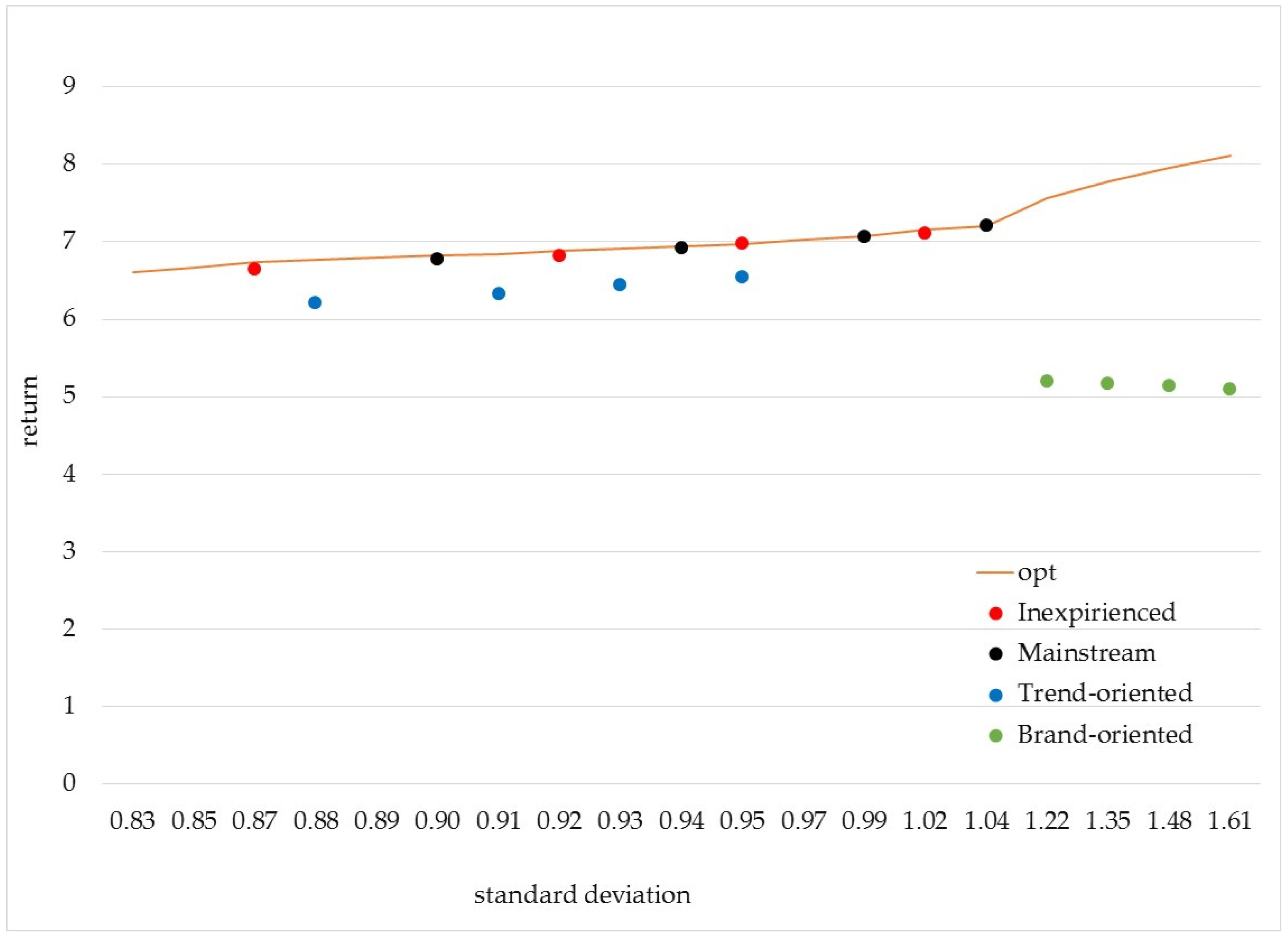
Diversification of the stocks for different levels of risk is similar in both approaches (Figure 4). Given that the risk level $(\sigma )$ in Table 10 already incrementally varies, diversifications were obtained directly from Table 8 and Table 9.

Finally, the comparison of the portfolios’ performance obtained using two approaches was performed for four identified segments. Risk $(\sigma )$ was calculated for each scale parameter and each segment, and the corresponding MMOPs were solved. The results were presented in the form of efficiency frontiers in Figure 5.

Figure 5 shows the efficiency frontier of optimization-based portfolios and the positions of preference-based returns relative to it.

6. Discussion

The aggregated DCA results have shown that dividend has the most significant influence on respondents’ preferences followed by trend of stock prices, while the company name and return rate have a much lower impact. Such results were expected as respondents were private investors. However, a great heterogeneity of the respondents’ preferences towards key stock characteristics was found and 4 clusters were isolated. Furthermore, an optimal portfolio based on preferences has been determined for the sample as a whole and for each segment. Portfolios were simulated for different values of the parameter reflecting the uncertainty of respondents’ responses.

The structure of portfolios obtained for all clusters but one (brand-oriented) are in line with Magron’s pyramidal approach. For example, low-risk stocks of Metalac a.d. are at the bottom of the pyramid with high shares, while the high-risk stocks of Energoprojekt holding are at the top with negligible shares, regardless of the values of the scale parameter. Such portfolios are in accordance with risk aversion of the majority of the sample. Moreover, performances of preference based portfolios are very close to the ones of the optimal portfolios obtained by using Markowitz approach, especially in the cases of mainstream and inexperienced segments. In addition to the fact that the return and risk of preference-based portfolios are close to the efficiency frontier, they also take into account preferences for particular companies that sometimes may be based on information about future business tendencies. Further, Markowitz’s approach considers risk relatively objectively—based on variance, while the discrete choice approach allows the impact of investor attitudes towards risk in the portfolio selection.

As for the whole-sample preference-based portfolios shown in Table 8, the share of Metalac a.d. is the largest in all four optimization-based portfolios (Table 10), followed by the shares of Nikola Tesla Airport, Jedinstvo a.d., and Energoprojekt holding. In addition, changes in the diversification of stocks with the increase of risk level have the same trend for all companies in both approaches: the share of Metalac a.d. increases while the shares of the other three companies decrease (Figure 4). The share values differ slightly in the two approaches, primarily because of preferences towards individual companies that influenced the respondents’ answers and were not taken into account in the optimization approach. This is particularly noticeable in the case of Nikola Tesla Airport, which ranks second in average preferences just behind Metalac a.d., but 20% of all respondents (members of the brand-oriented cluster) show strong preferences for that company (see Figure 2), which increases its overall share.

Table 9 indicates that Energoprojekt holding has a much lower dividend than other companies. Therefore, the share of its stocks in the preference-based portfolio is extremely small at the sample levels (0.5–1.8%). However, this company is negatively correlated with the remaining three companies (see Table 9) so it is not surprising that it has a larger share in the optimization-based portfolio (4.69–6.82%), despite the low level of dividend. However, with the increase of risk level $(\sigma )$, the share of Energoprojekt holding stocks decreases in optimal portfolios in both approaches (Figure 4).

Regarding efficiency frontiers in Figure 5, it can be seen that portfolios of mainstream and inexperienced segments are the closest to the optimization-based efficiency frontier, with the expected returns 0.018% and 0.052% lower (on average) than optimal, respectively. For each scale parameter (b), the inexperienced segment has a less risky portfolio than the mainstream segment, which is consistent with their lack of experience in stock market trading. These two segments comprise around 62% of the sample, which is close to the Pfiffelmann et al. [10] conclusion about the efficiency of BPT optimal portfolios, especially considering that the expected return of the third segment (trend-oriented) is on average only 0.49% lower than optimal. Portfolios of the trend-oriented segment are generally characterized by a risk lower than the portfolios of the previous two segments, which is in line with risk aversion of this segment’s respondents. Finally, portfolios of the brand-oriented segment are the most risky and have the lowest expected return since the respondents in this segment strongly prefer Nikola Tesla Airport regardless of other features of this company’s stocks.

7. Conclusions

The subject of this paper is the problem of portfolio selection and the importance of stock features for private investors. It is already shown in the behavioral finance literature that private investors consider other stock factors beyond Markowitz’s return rate and risk. In this paper, we have used discrete choice analysis to examine the preferences of private investors to four stocks’ attributes: return rate, risk expressed by the trend of the stock prices, dividend, and perception of the company.

The findings of this research are significant in both theoretical and practical terms. In theoretical terms, findings point to the importance of behavioral factors in investment decisions, thus enriching the existing scientific literature with a list of key influencing factors. When it comes to practical implications, the perceived importance of the brand in decision making gives companies an insight into the affinities of private investors and leads them to strengthen the brand of the company in the minds of investors.

The proposed methodology has several advantages since it:

• Corresponds with behavioral approach to portfolio selection and takes into account various portfolio performance indicators beyond risk and return;
• Incorporates risk attitude and subjective preferences towards portfolio selection criteria, both quantitative and qualitative, thus enabling identification of trade-offs that individuals are ready to make between conflicting criteria;
• Enables the collection of data on categories of respondents for which there are no historical data on stock market behavior.

The main weakness of proposed approach is its complexity as it requires extensive survey. The limitation of the particular study presented in this paper refers to the lack of verification on historical data related to private investors’ behavior on stock market. Moreover, only private investors’ preferences and attitudes were investigated and the sample was restricted to one region. Future research will be directed towards institutional investors’ preferences analysis, as well as to the application of the proposed approach to a larger set of companies. Such research could be more comprehensive in sense that includes a number of other portfolio criteria and involves the global population. It would also be useful to compare the results obtained by the proposed approach with the actual behavior of investors and to verify them based on the revealed preferences.