An Inequality Approach to Approximate Solutions of Set Optimization Problems in Real Linear Spaces

Abstract

This paper explores new notions of approximate minimality in set optimization using a set approach. We propose characterizations of several approximate minimal elements of families of sets in real linear spaces by means of general functionals, which can be unified in an inequality approach. As particular cases, we investigate the use of the prominent Tammer–Weidner nonlinear scalarizing functionals, without assuming any topology, in our context. We also derive numerical methods to obtain approximate minimal elements of families of finitely many sets by means of our obtained results.

1. Introduction

Set optimization has become an important research area and has gained tremendous interest within the optimization community due to its wide and important applications; see, e.g., [1,2,3,4]. There exist various research fields that directly lead to problems which can most satisfactorily be modeled and solved in the unified framework provided by set optimization. For example, duality in vector optimization, gap functions for vector variational inequalities, fuzzy optimization, as well as many problems in image processing, viability theory, economics etc. all lead to optimization problems that can be modeled as set-valued optimization problems. For an introduction to set optimization and its applications, we refer to [5].

For example, it is well known that uncertain optimization problems can be modeled by means of set optimization. Uncertainty here means that some parameters are not known. Instead, possibly only an estimated value or a set of possible values can be determined. As inaccurate data can have severe impacts on the model and therefore on the computed solution, it is important to take such uncertainty into account when modeling an optimization problem. If uncertainty is included in the optimization model, one is left with not only one objective function value, but possibly a whole set of values. This leads to a set-valued optimization problem, where the objective map is set-valued.

Recently, it has been shown that certain concepts of robustness for dealing with uncertainties in vector optimization can be described using approaches from set-valued optimization (see [2,3] and a practical application in the context of layout optimization of photovoltaic powerplants in [6]). The concept of interval arithmetic for computations with strict error bounds [7] is also a special case of dealing with set-valued mappings.

To obtain minimal solutions of a set-valued optimization problem, one must analyze whether one set dominates another set in a certain sense, i.e., by means of a given set relation. As it turns out, however, (depending on the chosen set relation), this intuitive and natural mathematical modeling framework often reaches its limitations and leads to very large or—even worse—empty solution sets. This is especially important throughout the design and implementation process of numerical algorithms for set optimization problems: The criteria involved in the definition of the set relations are usually based on set inclusions which for continuous problems are very sensitive to numerical inaccuracies or even just round-off errors.

A simple way to remedy this is to use approximate solution concepts: Here, the strict set inclusions are in a way relaxed by extending (enlarging/translating) the quantities that are to be compared such that one obtains more robust results for the involved inclusion tests.

The goal of this paper lies in the characterization of several well-known set relations by means of a very broad, manageable and easy-to-compute functional in the context of approximate solutions to set optimization problems using the set approach. In contrast to recent results in this area (for example see [8,9,10,11]), we assume that the spaces in which the sets are compared are not endowed with a particular topology. Therefore, our results generalize those found in the literature by dismissing topological properties. Please note that the references [10,11] present results on scalarizing functionals, but the functional acts on a real linear topological space and no relation to approximate solutions is presented there. Moreover, in [8,9], the oriented distance functional (which implicitly requires a topology) is used to derive characterizations of set relations. To the best of our knowledge, our approach of combining algebraic tools with approximate minimality notions in set optimization is original. That way, our results are not only valid in a broader mathematical setting but also provide some further insight into the purely algebraic tools and theoretical requirements necessary to acquire our findings. This is not only mathematically interesting, but deepens the theoretical understanding of approximate minimality in set optimization. It is furthermore in line with the recent increased interest in studying optimality conditions and separation concepts in spaces without a particular topology underneath it, see [12,13,14,15,16,17,18,19,20,21] and the references therein.

2. Preliminaries

Throughout this work, let Y be a real linear space. Following the nomenclature of [22], for a nonempty set $F\subseteq Y$, we denote by

$$coreF:=\{y\in Y|\forall v\in Y\exists \lambda >0\mathrm{s}.\mathrm{t}.y+[0,\lambda ]v\subseteq F\}$$

the algebraic interior of F and for any given $k\in Y$, let

$${vcl}_{k}F:=\{y\in Y|\forall \lambda >0\exists {\lambda }^{\prime }\in [0,\lambda ]\mathrm{s}.\mathrm{t}.y+{\lambda }^{\prime }k\in F\}.$$

We say that F is k-vectorially closed if ${vcl}_{k}F=F$. Obviously, it holds $F\subseteq {vcl}_{k}F$ for all $k\in Y$.

We denote by $\mathcal{P}\left(Y\right):=\{A\subseteq Y|A\mathrm{is}\mathrm{nonempty}\}$ the power set of Y without the empty set. For two elements A, B of $\mathcal{P}\left(Y\right)$, we denote the sum of sets by

$$A+B:=\{a+b|a\in A,b\in B\}.$$

The set $F\subseteq Y$ is a cone if for all $f\in F$ and $\lambda \ge 0$, $\lambda f\in F$ holds true. The cone F is convex if $F+F\subseteq F$.

Now let $\varnothing \ne C\subseteq Y$ and $k\in Y\backslash \left\{0\right\}$. We recall the functional $z^{C,k}:Y\to \mathbb{R}\cup \{+\infty \}\cup \{-\infty \}=:\overline{\mathbb{R}}$ from Gerstewitz [23] (which has very recently been extended to the space Y without assuming any topology, see [24] and the references therein)

$$z^{C,k}\left(y\right):=\left\{\begin{array}{cc}+\infty \hfill & \mathrm{if}y\notin \mathbb{R}k-C,\hfill \\ inf\{t\in \mathbb{R}|y\in tk-C\}\hfill & \mathrm{otherwise}.\hfill \end{array}\right.$$

(1)

The functional $z^{C,k}$ was originally introduced as scalarizing functional in vector optimization. Please note that the construction of $z^{C,k}$ was mentioned by Krasnosel’skiĭ [25] (see Rubinov [26]) in the context of operator theory. Figure 1 visualizes the functional $z^{C,k}$, where $C={\mathbb{R}}_{+}^2$ has been taken as the natural ordering cone in ${\mathbb{R}}^2$ and $k\in coreC$. We can see that the set $-C$ is moved along the line $\mathbb{R}·k$ up until y belongs to $tk-C$. The functional $z^{C,k}$ assigns the smallest value t such that the property $y\in tk-C$ is fulfilled.

The functional $z^{C,k}$ plays an important role as nonlinear separation functional for not necessarily convex sets. Applications of $z^{C,k}$ include coherent risk measures in financial mathematics (see, for instance, [27]) and uncertain programming (see [2,3]). Several important properties of $z^{C,k}$ (in the case that Y is endowed with a topology) were studied in [28,29]. Now let us recall the definition of E-monotonicity of a functional.

Definition 1.

Let $E\in \mathcal{P}\left(Y\right)$. A functional $z:Y\to \overline{\mathbb{R}}$ is called E-monotoneif

$$y_1,y_2\in Y:y_1\in y_2-E\Rightarrow z\left(y_1\right)\le z\left(y_2\right).$$

Below we provide some properties of the functional $z^{C,k}$ introduced in (1).

Proposition 1

([22]). Let C and E be nonempty subsets of Y, and let $k\in Y\backslash \left\{0\right\}$. Then the following properties hold.

(a) 

$\forall y\in Y:z^{C,k}\left(y\right)\le 0$⟺$y\in (-\infty ,0]k-{vcl}_{k}C$.

(b) 

$\forall y\in Y:z^{C,k}\left(y\right)<0$⟺$y\in (-\infty ,0)k-{vcl}_{k}C$.

(c) 

$z^{C,k}$ is E-monotone if and only if $E+C\subset [0,+\infty )k+{vcl}_{k}C$.

(d) 

$\forall y\in Y,\forall r\in \mathbb{R}:$$z^{C,k}(y+rk)=z^{C,k}\left(y\right)+r$.

The set relations to be defined below rely on set inclusions where the set C is attached pointwise to the considered sets $A,B\in \mathcal{P}\left(Y\right)$. The following corollary relates $A+C$ and $A-C$ respectively by means of the functional $z^{C,k}$ in the case that C is a convex cone.

Corollary 1

([14], Corollary 2.3). Let $C\subseteq Y$ be a convex cone, $A\in \mathcal{P}\left(Y\right)$ and $k\in Y\backslash \left\{0\right\}$. Then it holds

$$\underset{a\in A}{sup}{z}^{C,k}\left(a\right)=\underset{y\in A-C}{sup}{z}^{C,k}\left(y\right)and\underset{a\in A}{inf}{z}^{C,k}\left(a\right)=\underset{y\in A+C}{inf}{z}^{C,k}\left(y\right).$$

A well-known set relation is the upper set less order relation introduced by Kuroiwa [30,31]. We recall a generalized version of this relation here, where the underlying set C is not necessarily a convex cone and thus the resulting relation is not necessarily an order.

Definition 2

(Upper Set Less Relation, [32]). Let $C\subseteq Y$. The upper set less relation ${⪯}_C^u$ is defined for two sets $A,B\in \mathcal{P}\left(Y\right)$ by

$$A{⪯}_C^{u}B:⟺A\subseteq B-C.$$

The following theorem shows a first connection between the upper set less relation and the nonlinear scalarizing functional $z^{C,k}$.

Theorem 1

([14], Theorem 3.2). Let $C\subseteq Y$ be a convex cone, $A,B\in \mathcal{P}\left(Y\right)$ and $k\in Y\backslash \left\{0\right\}$. Then

$$A{⪯}_C^{u}B⟹\underset{a\in A}{sup}{z}^{C,k}\left(a\right)\le \underset{b\in B}{sup}{z}^{C,k}\left(b\right).$$

The converse implication in Theorem 1 is not generally fulfilled, even if the underlying sets are convex, see ([33], Example 3.2). However, we have the following result.

Theorem 2

([14], Theorem 3.3). Let $C\subseteq Y$. For two sets $A,B\in \mathcal{P}\left(Y\right)$ and $k\in Y\backslash \left\{0\right\}$, it holds

$$A{⪯}_C^{u}B⟹\underset{a\in A}{sup}\underset{b\in B}{inf}{z}^{C,k}(a-b)\le 0.$$

Assume on the other hand that there exists a $k_0\in Y\backslash \left\{0\right\}$ such that ${inf}_{b\in B}{z}^{C,k_0}(a-b)$ is attained for all $a\in A$, C is $k_0$-vectorially closed and $[0,+\infty )k_0+C\subseteq C$. Then

$$\underset{a\in A}{sup}\underset{b\in B}{inf}{z}^{C,k_0}(a-b)\le 0⟹A{⪯}_C^{u}B.$$

Remark 1.

(1) 

Please note that for any $A,B\in \mathcal{P}\left(Y\right)$, the set relation $A{⪯}_C^{u}B$ by Theorem 2 also implies ${sup}_{k\in Y\backslash \left\{0\right\}}{sup}_{a\in A}{inf}_{b\in B}{z}^{C,k}(a-b)\le 0$.

(2) 

Let $A,B\in \mathcal{P}\left(Y\right)$ and $C\subseteq Y$. If there exists an element $k_0\in C\backslash \left\{0\right\}$ such that ${inf}_{b\in B}{z}^{C,k_0}(a-b)$ is attained for all $a\in A$, C is $k_0$-vectorially closed and $[0,+\infty )k_0+C=C$, then it follows from Theorem 2 that

$$\begin{array}{cc}\hfill A{⪯}_C^{u}B& ⟺\underset{a\in A}{sup}\underset{b\in B}{inf}{z}^{C,k_0}(a-b)\le 0\hfill \\ \hfill & ⟺\underset{k\in Y\backslash \left\{0\right\}}{sup}\underset{a\in A}{sup}\underset{b\in B}{inf}{z}^{C,k}(a-b)\le 0.\hfill \end{array}$$

In the second part of Theorem 2, we need the assumption that there exists a $k_0\in Y\backslash \left\{0\right\}$ such that ${inf}_{b\in B}{z}^{C,k_0}(a-b)$ is attained for all $a\in A$. Sufficient conditions for such an attainment property, i.e., assertions concerning the existence of solutions of the corresponding optimization problems (extremal principles) are given in the literature. The well-known Theorem of Weierstrass says that a lower semi-continuous function on a nonempty weakly compact set in a reflexive Banach space has a minimum. An extension of the Theorem of Weierstrass is given by Zeidler ([34], Proposition 9.13): A proper lower semi-continuous and quasi-convex function on a nonempty closed bounded convex subset of a reflexive Banach space has a minimum. Since the functional $z^{C,k_0}$ is studied here in the context of real linear spaces that are not endowed with a particular topology, we cannot rely on continuity assumptions. Therefore, we propose the following theorem without any attainment property.

Theorem 3

([14], Theorem 3.6). Let $C\subseteq Y$, $A,B\in \mathcal{P}\left(Y\right)$ and $k_0\in Y\backslash \left\{0\right\}$ such that $(-\infty ,0)k_0-{vcl}_{k_0}C\subseteq -C$ and ${vcl}_{-k_0}(B-C)\subseteq B-C$. Then

$$\underset{a\in A}{sup}\underset{b\in B}{inf}{z}^{C,k_0}(a-b)\le 0⟹A{⪯}_C^{u}B.$$

We also consider the following set relation, which compares sets based on their lower bounds (compare [30,31] for the according definition for orders).

Definition 3

(Lower Set Less Relation, [32]). Let $C\subseteq Y$. The lower set less relation ${⪯}_C^l$ is defined for two sets $A,B\in \mathcal{P}\left(Y\right)$ by

$$A{⪯}_C^{l}B:⟺B\subseteq A+C.$$

Because $A{⪯}_C^{u}B$ is equivalent to $-B{⪯}_C^l-A$, we obtain the following corollaries from Theorems 1, 2 and 3.

Corollary 2

([14], Corollary 3.9). Let $C\subseteq Y$ be a convex cone, $A,B\in \mathcal{P}\left(Y\right)$ and $k\in Y\backslash \left\{0\right\}$. Then

$$A{⪯}_C^{l}B⟹\underset{a\in A}{inf}{z}^{C,k}\left(a\right)\le \underset{b\in B}{inf}{z}^{C,k}\left(b\right).$$

Corollary 3

([14], Corollary 3.10). Let $C\subseteq Y$. For two sets $A,B\in \mathcal{P}\left(Y\right)$ and $k\in Y\backslash \left\{0\right\}$, it holds

$$A{⪯}_C^{l}B⟹\underset{b\in B}{sup}\underset{a\in A}{inf}{z}^{C,k}(a-b)\le 0.$$

Assume on the other hand that there exists a $k_0\in Y\backslash \left\{0\right\}$ such that ${inf}_{a\in A}{z}^{C,k_0}(a-b)$ is attained for all $b\in B$, C is $k_0$-vectorially closed and $[0,+\infty )k_0+C\subseteq C$. Then

$$\underset{b\in B}{sup}\underset{a\in A}{inf}{z}^{C,k_0}(a-b)\le 0⟹A{⪯}_C^{l}B.$$

Corollary 4

([14], Corollary 3.11). Let $C\subseteq Y$, $A,B\in \mathcal{P}\left(Y\right)$ and $k_0\in Y\backslash \left\{0\right\}$ such that $(-\infty ,0)k_0-{vcl}_{k_0}C\subseteq -C$ and ${vcl}_{-k_0}(A-C)\subseteq -A-C$. Then

$$\underset{b\in B}{sup}\underset{a\in A}{inf}{z}^{C,k_0}(a-b)\le 0⟹A{⪯}_C^{l}B.$$

We also study the so-called set less relation (see [35,36] for the case where the underlying set C is a convex cone).

Definition 4

(Set Less Relation, [32]). Let $C\subseteq Y$. The set less relation ${⪯}_C^s$ is defined for two sets $A,B\in \mathcal{P}\left(Y\right)$ by

$$A{⪯}_C^{s}B:⟺A{⪯}_C^{u}BandA{⪯}_C^{l}B.$$

We immediately obtain the following results.

Corollary 5

([14], Corollary 3.13). Let $C\subseteq Y$ be a convex cone, $A,B\in \mathcal{P}\left(Y\right)$ and $k\in Y\backslash \left\{0\right\}$. Then

$$A{⪯}_C^{s}B⟹\underset{a\in A}{sup}{z}^{C,k}\left(a\right)\le \underset{b\in B}{sup}{z}^{C,k}\left(b\right)and\underset{a\in A}{inf}{z}^{C,k}\left(a\right)\le \underset{b\in B}{inf}{z}^{C,k}\left(b\right).$$

Corollary 6

([14], Corollary 3.14). Let $C\subseteq Y$. For two sets $A,B\in \mathcal{P}\left(Y\right)$ and $k\in Y\backslash \left\{0\right\}$, it holds

$$A{⪯}_C^{s}B⟹\underset{a\in A}{sup}\underset{b\in B}{inf}{z}^{C,k}(a-b)\le 0and\underset{b\in B}{sup}\underset{a\in A}{inf}{z}^{C,k}(a-b)\le 0.$$

Assume on the other hand that there exists a $k_0\in Y\backslash \left\{0\right\}$ such that ${inf}_{b\in B}{z}^{C,k_0}(a-b)$ is attained for all $a\in A$, and there exists $k_1\in Y\backslash \left\{0\right\}$ such that ${inf}_{a\in A}{z}^{C,k_1}(a-b)$ is attained for all $b\in B$, C is both $k_0$- and $k_1$-vectorially closed, $[0,+\infty )k_0+C\subseteq C$ and $[0,+\infty )k_1+C\subseteq C$. Then

$$\underset{a\in A}{sup}\underset{b\in B}{inf}{z}^{C,k_0}(a-b)\le 0and\underset{b\in B}{sup}\underset{a\in A}{inf}{z}^{C,k_1}(a-b)\le 0⟹A{⪯}_C^{s}B.$$

Corollary 7

([14], Corollary 3.15). Let $C\subseteq Y$, $A,B\in \mathcal{P}\left(Y\right)$ and $k_0,k_1\in Y\backslash \left\{0\right\}$ such that $(-\infty ,0)k_0-{vcl}_{k_0}C\subseteq -C$, $(-\infty ,0)k_1-{vcl}_{k_1}C\subseteq -C$, ${vcl}_{-k_0}(B-C)\subseteq B-C$ and ${vcl}_{-k_1}(A-C)\subseteq A-C$. Then

$$\underset{a\in A}{sup}\underset{b\in B}{inf}{z}^{C,k_0}(a-b)\le 0and\underset{b\in B}{sup}\underset{a\in A}{inf}{z}^{C,k_1}(a-b)\le 0⟹A{⪯}_C^{s}B.$$

3. Approximate Minimal Elements of Set Optimization Problems

The following definition describes minimality in the setting of a family of sets (see ([5], Definition 2.6.19) for the corresponding definition for preorders).

Definition 5

(Minimal Elements). Let $\mathcal{A}$ be a family of elements of $\mathcal{P}\left(Y\right)$. $\overline{A}\in \mathcal{A}$ is called a minimal element of $\mathcal{A}$ w. r. t. ⪯ if

$$A⪯\overline{A},A\in \mathcal{A}⟹\overline{A}⪯A.$$

The set of all minimal elements of $\mathcal{A}$ w. r. t. ⪯ will be denoted by ${\mathcal{A}}_{min}$.

Please note that if the elements of $\mathcal{A}$ are single-valued and $A⪯\overline{A}:⟺A\in \overline{A}-C$ with $C\subseteq Y$ being a convex cone, then Definition 5 reduces to the standard notion of minimality in vector optimization (compare, for example, ([15], Definition 4.1)). From vector optimization, it is well known that usually, the existence of minimal elements can only be guaranteed under additional assumptions (for an existence result of minimal elements in set optimization, see, for example, [37]). Since the set ${\mathcal{A}}_{min}$ may be empty, it is common practice to use a weaker notion of minimality, so-called approximate minimality. For this reason, we extend three notions of approximate minimality that were originally introduced in [38]. In [38], the following definitions are given for $⪯={⪯}_C^l$ (see Definition 3). In order to stay as general as possible, we define approximate minimality using set relations that are not required to possess any ordering structure.

Definition 6.

Let $\mathcal{A}$ be a family of elements of $\mathcal{P}\left(Y\right)$, $H\in \mathcal{P}\left(Y\right)$, $H\ne Y$ and ⪯ be a binary relation on $\mathcal{A}$.

(a) 

$\overline{A}\in \mathcal{A}$ is called an $H^1$–approximate minimal element of $\mathcal{A}$ w. r. t. ⪯ if

$$A⪯\overline{A},A\in \mathcal{A}⟹\overline{A}⪯A+H.$$

(b) 

$\overline{A}\in \mathcal{A}$ is called an $H^2$–approximate minimal element of $\mathcal{A}$ w. r. t. ⪯ if

$$A+H⪯\overline{A},A\in \mathcal{A}⟹\overline{A}⪯A+H.$$

(c) 

$\overline{A}\in \mathcal{A}$ is called an $H^3$–approximate minimal element of $\mathcal{A}$ w. r. t. ⪯ if $A+H\cancel{⪯}\overline{A}$, for all $A\in \mathcal{A}\backslash \overline{A}$.

The set of all $H^i$–approximate minimal elements of $\mathcal{A}$ w. r. t. ⪯ ($i=1,2,3$) will be denoted by ${\mathcal{A}}_{H^i}$.

Please note that Definition 6 (a) is a natural formulation for approximate minimality, while Definition 6 (b) is derived from the standard notion of approximate efficiency for vector-valued maps (see ([38], Remark 2.5)). Definition 6 (c) represents an approximate version of the well-known nondomination concept of vector optimization.

Here we consider a set-valued optimization problem in the following setting: Let $S\subseteq {\mathbb{R}}^n$, a set-valued mapping $F:S\rightrightarrows Y$ and a set relation ⪯ be given. We are looking for approximate minimal elements w. r. t. the order relation ⪯ in the sense of Definition 6 of the problem

$$\underset{x\in S}{min}F\left(x\right).$$

(2)

We say that $\overline{x}\in S$ is an $H^i$–approximate minimal solution ($i=1,2,3$) of (2) w. r. t. ⪯ if $F\left(\overline{x}\right)$ is an $H^i$–approximate minimal element of the family of sets $F\left(x\right)$, $x\in S$ w. r. t. ⪯. The family of sets $F\left(x\right)$, $x\in S$, is denoted by $\mathcal{A}$.

Now we will present characterizations of approximate minimal solutions of (2) w. r. t. ⪯. In what follows, we will use the following notation. For some $\overline{x}\in S$, let us denote

$${\left[F\left(\overline{x}\right)\right]}_{⪯}^{H^1}:=\left\{x\in S|F\left(x\right)⪯F\left(\overline{x}\right),F\left(\overline{x}\right)⪯F\left(x\right)+H\right\}$$

and

$${\left[F\left(\overline{x}\right)\right]}_{⪯}^{H^2}:=\left\{x\in S|F\left(x\right)+H⪯F\left(\overline{x}\right),F\left(\overline{x}\right)⪯F\left(x\right)+H\right\}.$$

The following proposition will be useful in the theorem below.

Proposition 2.

$\overline{x}\in S$ is an $H^1$-approximate minimal solution of the problem (2) w. r. t. ⪯ if and only if for any $x\in S\backslash {\left[F\left(\overline{x}\right)\right]}_{⪯}^{H^1}$, we have $F\left(x\right)\cancel{⪯}F\left(\overline{x}\right)$.

Proof. 

First note that $x\in S\backslash {\left[F\left(\overline{x}\right)\right]}_{⪯}^{H^1}$ means that $x\in S$ such that $F\left(x\right)\cancel{⪯}F\left(\overline{x}\right)$ or $F\left(\overline{x}\right)\cancel{⪯}F\left(x\right)+H$. Let $\overline{x}\in S$ be an $H^1$-approximate minimal solution of the problem (2) w. r. t. ⪯. Then we must consider two cases:

Case 1: 

For $x\in S$ and $F\left(x\right)\cancel{⪯}F\left(\overline{x}\right)$, there is nothing left to show.

Case 2: 

For $x\in S$ and $F\left(\overline{x}\right)\cancel{⪯}F\left(x\right)+H$, we obtain $F\left(x\right)\cancel{⪯}F\left(\overline{x}\right)$ due to $\overline{x}$’s $H^1$-approximate minimality, as desired.

Conversely, assume that for all $x\in S\backslash {\left[F\left(\overline{x}\right)\right]}_{⪯}^{H^1}$, $F\left(x\right)\cancel{⪯}F\left(\overline{x}\right)$ holds true. Suppose, by contradiction, that $\overline{x}$ is not an $H^1$-approximate minimal solution of the problem (2) w. r. t. ⪯. This implies the existence of some $x\in S$ with the properties $F\left(x\right)⪯F\left(\overline{x}\right)$ and $F\left(\overline{x}\right)\cancel{⪯}F\left(x\right)$, in contradiction to the assumption. □

Now we consider a functional $g^{H^1}:S\times S\to \mathbb{R}\cup \{\pm \infty \}$ with the property

$$\forall x,\overline{x}\in S:g^{H^1}(x,\overline{x})\le 0⟺F\left(x\right)⪯F\left(\overline{x}\right).$$

Then we have the following characterization for $H^1$-approximate minimal solution of the problem (2) w. r. t. ⪯.

Theorem 4.

$\overline{x}\in S$ is an $H^1$-approximate minimal solution of the problem (2) w. r. t. ⪯ if and only if the following system (in the unknown x)

$$\begin{array}{c}\hfill g^{H^1}(x,\overline{x})\le 0,x\in S\backslash {\left[F\left(\overline{x}\right)\right]}_{⪯}^{H^1},\end{array}$$

is impossible.

Proof. 

First note that due to Proposition 2, $\overline{x}\in S$ is an $H^1$-approximate minimal solution of the problem (2) w. r. t. ⪯ if and only if for $x\in S\backslash {\left[F\left(\overline{x}\right)\right]}_{⪯}^{H^1}$, we have $F\left(x\right)\cancel{⪯}F\left(\overline{x}\right)$. Furthermore, we have

$$\begin{array}{cc}\hfill g^{H^1}(x,\overline{x})\le 0,& x\in S\backslash {\left[F\left(\overline{x}\right)\right]}_{⪯}^{H^1}\mathrm{is}\mathrm{impossible}\hfill \\ \hfill & ⟺\nexists x\in S\backslash {\left[F\left(\overline{x}\right)\right]}_{⪯}^{H^1}:g^{H^1}(x,\overline{x})\le 0\hfill \\ \hfill & ⟺\forall x\in S\backslash {\left[F\left(\overline{x}\right)\right]}_{⪯}^{H^1}:g^{H^1}(x,\overline{x})>0\hfill \\ \hfill & ⟺\forall x\in S\backslash {\left[F\left(\overline{x}\right)\right]}_{⪯}^{H^1}:F\left(x\right)\cancel{⪯}F\left(\overline{x}\right).\hfill \end{array}$$

 □

In a similar manner as Proposition 2 and Theorem 4, one can verify the following results. For this, we assume that we are given a functional $g^{H^2}:S\times S\to \mathbb{R}\cup \{\pm \infty \}$ with the property

$$\forall x,\overline{x}\in S:g^{H^2}(x,\overline{x})\le 0⟺F\left(x\right)+H⪯F\left(\overline{x}\right).$$

Proposition 3.

$\overline{x}\in S$ is an $H^2$-approximate minimal solution of the problem (2) w. r. t. ⪯ if and only if for any $x\in S\backslash {\left[F\left(\overline{x}\right)\right]}_{⪯}^{H^2}$, we have $F\left(x\right)+H\cancel{⪯}F\left(\overline{x}\right)$.

Theorem 5.

$\overline{x}\in S$ is an $H^2$-approximate minimal solution of the problem (2) w. r. t. ⪯ if and only if the following system (in the unknown x)

$$\begin{array}{c}\hfill g^{H^2}(x,\overline{x})\le 0,x\in S\backslash {\left[F\left(\overline{x}\right)\right]}_{⪯}^{H^2},\end{array}$$

is impossible.

Let us now consider problem (2) with the set relation $⪯={⪯}_C^u$. Motivated by Theorem 3 and Corollary 4 above, we consider the functionals $g_u^{H^i}:S\times S\to \mathbb{R}\cup \{\pm \infty \}$ ($i=1,2$) defined by

$$\begin{array}{cc}\hfill g_u^{H^1}(x,\overline{x})& :=\underset{y\in F\left(x\right)}{sup}\underset{\overline{y}\in F\left(\overline{x}\right)}{inf}{z}^{C,k}(y-\overline{y}),\hfill \\ \hfill g_u^{H^2}(x,\overline{x})& :=\underset{y\in F\left(x\right)+H}{sup}\underset{\overline{y}\in F\left(\overline{x}\right)}{inf}{z}^{C,k}(y-\overline{y}).\hfill \end{array}$$

Assumption 1.

For $C\subseteq Y$, $k\in Y\backslash \left\{0\right\}$, and $\overline{x}\in S$ we assume that

(a-H¹) 

C is k-vectorially closed, $[0,+\infty )k+C\subseteq C$, and for all $x\in S\backslash {\left[F\left(\overline{x}\right)\right]}_{{⪯}_C^u}^{H^1}$ and $y\in F\left(x\right)$, the infimum ${inf}_{\overline{y}\in F\left(\overline{x}\right)}{z}^{C,k}(y-\overline{y})$ is attained;

(a-H²) 

C is k-vectorially closed, $[0,+\infty )k+C\subseteq C$, and for all $x\in S\backslash {\left[F\left(\overline{x}\right)\right]}_{{⪯}_C^u}^{H^2}$ and $y\in F\left(x\right)+H$, the infimum ${inf}_{\overline{y}\in F\left(\overline{x}\right)}{z}^{C,k}(y-\overline{y})$ is attained;

(b) 

$(-\infty ,0)k-{vcl}_{k}C\subseteq -C$ and ${vcl}_{-k}(F\left(\overline{x}\right)-C)\subseteq F\left(\overline{x}\right)-C$.

We next present a sufficient and necessary condition for $H^1$-approximate minimal solutions of the problem (2) w. r. t. the relation ${⪯}_C^u$.

Corollary 8.

Let Assumption 1 (a-$H^i$) or (b) be satisfied. Then $\overline{x}\in S$ is an $H^i$-approximate minimal solution ($i=1,2$) of the problem (2) w. r. t. ${⪯}_C^u$ if and only if the following system (in the unknown x)

$$\begin{array}{c}\hfill g_u^{H^i}(x,\overline{x})\le 0,x\in S\backslash {\left[F\left(\overline{x}\right)\right]}_{{⪯}_C^u}^{H^i},\end{array}$$

is impossible.

Proof. 

The proof follows by Theorems 2, 3, 4 and 5. □

Furthermore, let us consider problem (2) with $⪯={⪯}_C^l$. We define the functions $g_l^{H^i}:S\times S\to \mathbb{R}\cup \{\pm \infty \}$ for $i=1,2$ by

$$\begin{array}{cc}\hfill g_l^{H^1}(x,\overline{x})& :=\underset{\overline{y}\in F\left(\overline{x}\right)}{sup}\underset{y\in F\left(x\right)}{inf}{z}^{C,k}(y-\overline{y})\hfill \\ \hfill g_l^{H^2}(x,\overline{x})& :=\underset{\overline{y}\in F\left(\overline{x}\right)}{sup}\underset{y\in F\left(x\right)+H}{inf}{z}^{C,k}(y-\overline{y}).\hfill \end{array}$$

Assumption 2.

For $C\subseteq Y$, $k\in Y\backslash \left\{0\right\}$, and $\overline{x}\in S$ we assume that

(a-H¹) 

C is k-vectorially closed, $[0,+\infty )k+C\subseteq C$, and for all $x\in S\backslash {\left[F\left(\overline{x}\right)\right]}_{{⪯}_C^l}^{H^1}$ and $\overline{y}\in F\left(\overline{x}\right)$, the infimum ${inf}_{y\in F\left(x\right)}{z}^{C,k}(y-\overline{y})$ is attained;

(a-H²) 

C is k-vectorially closed, $[0,+\infty )k+C\subseteq C$, and for all $x\in S\backslash {\left[F\left(\overline{x}\right)\right]}_{{⪯}_C^l}^{H^2}$ and $\overline{y}\in F\left(\overline{x}\right)$, the infimum ${inf}_{y\in F\left(x\right)+H}{z}^{C,k}(y-\overline{y})$ is attained;

(b) 

$(-\infty ,0)k-{vcl}_{k}C\subseteq -C$ and for all $x\in S:{vcl}_{-k}(-F\left(x\right)-C)=-F\left(x\right)-C$.

In the following, we present a sufficient and necessary condition for $H^i$-approximate minimal solutions of the problem (2) w. r. t. ${⪯}_C^l$.

Corollary 9.

Let Assumption 2 (a-$H^i$) or (b) be satisfied. Then $\overline{x}$ is an $H^i$-approximate minimal solution ($i=1,2$) of the problem (2) w. r. t. ${⪯}_C^l$ if and only if the following system (in the unknown x)

$$\begin{array}{c}\hfill g_l^{H^1}(x,\overline{x})\le 0,x\in S\backslash {\left[F\left(\overline{x}\right)\right]}_{{⪯}_C^l}^{H^i},\end{array}$$

is impossible.

Proof. 

The proof follows by Corollaries 3 and 4 as well as Theorems 4 and 5. □

Finally, we have the following result for $H^i$-approximate minimal solutions of the problem (2) w. r. t. ${⪯}_C^s$.

Corollary 10.

Let $i\in \{1,2\}$ and suppose that Assumptions 1 (a-$H^i$) and 2 (a-$H^i$) or Assumptions 1 (b) and 2 (b) are satisfied for the same $k\in Y\backslash \left\{0\right\}$. Then $\overline{x}$ is an $H^i$-approximate minimal solution of the problem (2) w. r. t. ${⪯}_C^s$ if and only if the following system (in the unknown x):

$$\begin{array}{c}\hfill g_u^{H^i}(x,\overline{x})\le 0and{g}_l^{H^i}(x,\overline{x})\le 0,x\in S\backslash \left({\left[F\left(\overline{x}\right)\right]}_{{⪯}_C^u}^{H^i}\cup {\left[F\left(\overline{x}\right)\right]}_{{⪯}_C^l}^{H^i}\right),\end{array}$$

is impossible.

4. Numerical Procedure for Computing ${\mathit{H}}^{\mathit{i}}$-Approximate Minimal Elements of a Family of Finitely Many Elements

Finding $H^i$-approximate minimal elements of a family of finitely many elements of $\mathcal{P}\left(Y\right)$ is very important. A first approach to deriving and implementing numerical methods for obtaining $H^i$-approximate minimal elements has been presented in [38] for the lower set less relation ${⪯}_C^l$. The assumption that the given family is finitely valued is oftentimes not a restriction, as many continuous set optimization problem can be appropriately discretized, see the discussion in [39] and the theoretical investigations for linear programs [40] as well as the numerical studies in [41]. In this section, we propose numerical methods for obtaining approximate minimal elements as proposed in Definition 5 for general set relations under suitable assumptions.

Please note that the following algorithms can be found in [38] for the specific case that the set relation is equal to ${⪯}_C^l$. We present them here for general set relations ⪯. The following algorithm is an extension of the so-called Graef-Younes method [42,43] and it is useful for sorting out elements which do not belong to the set of $H^i$–approximate minimal elements.

Algorithm 1: (Method for sorting out elements of a family of finitely many sets which are not $H^1$- ($H^2$-, $H^3$-, respectively) approximate minimal elements).

Input:$\mathcal{A}:=\{A_1,\dots ,A_m\}$, set relation ⪯, $H\in \mathcal{P}\left(Y\right)$

% initialization

$\mathcal{T}:=\left\{A_1\right\}$,

% iteration loop

for$j=2:1:m$do

if $\left(A⪯A_j,A\in \mathcal{T}⟹A_j⪯A+H\right)$

$(\left(A+H⪯A_j,A\in \mathcal{T}⟹A_j⪯A+H\right)$, respectively$)$,

$(A+H\cancel{⪯}\overline{A}$, $A\in \mathcal{T}$, respectively$)$, then

$\mathcal{T}:=\mathcal{T}\cup \left\{A_j\right\}$

end if

end for

Output:$\mathcal{T}$

Remark 2.

1. 

Please note that the if-condition in Algorithm 1 is usually not implemented straightforwardly but instead an additional loop over the elements of the set $\mathcal{T}$ is performed. We nevertheless use the above notation of this step to be consistent with the literature on algorithms of Graef-Younes type.

2. 

Note also that the if-condition describes approximate minimality in the set $\mathcal{T}$. Therefore, Definition 6 does not have to be applied to the whole set $\mathcal{A}$, but to a smaller set $\mathcal{T}$, which can drastically reduce the numerical effort. In this way, non-approximate minimal elements can be eliminated from the set $\mathcal{A}$, as the following theorem shows.

Theorem 6.

1. 

Algorithm 1 is well-defined.

2. 

Algorithm 1 generates a nonempty set $\mathcal{T}\subseteq \mathcal{A}$.

3. 

Every $H^1$- ($H^2$-, $H^3$-, respectively) approximate minimal element of $\mathcal{A}$ w. r. t. ⪯ also belongs to the set $\mathcal{T}$ generated by Algorithm 1.

Proof. 

The statements 1 and 2 are easily checked (We loop over a finite number of elements, all the necessary comparisons are well-defined and after the first step, the set $\mathcal{T}$ already consists of an element.) and therefore, their proofs are omitted. Now let $A_j$ be an $H^1$- ($H^2$-, $H^3$-, respectively) approximate minimal element of $\mathcal{A}$. Then we have

$$\begin{array}{c}A⪯A_j,A\in \mathcal{A}⟹A_j⪯A+H\hfill \\ (A+H⪯A_j,A\in \mathcal{A}⟹A_j⪯A+H,\mathrm{respectively}),\hfill \\ (A+H\cancel{⪯}\overline{A},A\in \mathcal{A},\mathrm{respectively}).\hfill \end{array}$$

Because of $\mathcal{T}\subseteq \mathcal{A}$, by the above implications we directly obtain

$$\begin{array}{c}A⪯A_j,A\in \mathcal{T}⟹A_j⪯A+H\hfill \\ (A+H⪯A_j,A\in \mathcal{T}⟹A_j⪯A+H,\mathrm{respectively}),\hfill \\ (A+H\cancel{⪯}{A}_j,A\in \mathcal{T},\mathrm{respectively}).\hfill \end{array}$$

which verifies that the if-condition in Algorithm 1 is satisfied and $A_j$ is added to $\mathcal{T}$. □

After the application of Algorithm 1 we have only created a smaller set $\mathcal{T}$ containing all the approximate minimal elements of the original family of sets. To filter out solely the approximate minimal elements, another step is required which we handle in the following algorithm:

Algorithm 2: (Method for finding $H^1$- ($H^2$-, $H^3$-, respectively) approximate minimal elements of a family $\mathcal{A}$ of finitely many sets).

Input:${\mathcal{A}}^{*}:=\{A_1,\dots ,A_m\}$, set relation ⪯, $H\in \mathcal{P}\left(Y\right)$

% initialization

$\mathcal{T}:=\left\{A_1\right\}$

% forward iteration loop

for$j=2:1:m$do

if $\left(A⪯A_j,A\in \mathcal{T}⟹A_j⪯A+H\right)$

$(\left(A+H⪯A_j,A\in \mathcal{T}⟹A_j⪯A+H\right)$,

$(A+H\cancel{⪯}{A}_j$, $A\in \mathcal{T}$, respectively$)$, then

$\mathcal{T}:=\mathcal{T}\cup \left\{A_j\right\}$

end if

end for

$\{A_1,\dots ,A_p\}:=\mathcal{T}$

$\mathcal{U}:=\left\{A_p\right\}$

% backward iteration loop

for$j=p-1:-1:1$do

if $\left(A⪯A_j,A\in \mathcal{U}⟹A_j⪯A+H\right)$

$(\left(A+H⪯A_j,A\in \mathcal{U}⟹A_j⪯A+H\right)$,

$(A+H\cancel{⪯}{A}_j$, $A\in \mathcal{U}$, respectively$)$, then

$\mathcal{U}:=\mathcal{U}\cup \left\{A_j\right\}$

end if

end for

Output:$\mathcal{U}$

$\{A_1,\dots ,A_q\}:=\mathcal{U}$

$\mathcal{V}:=\varnothing$

% final comparison

for$j=1:1:q$do

if $\left(A⪯A_j,A\in \mathcal{A}\backslash \mathcal{U}⟹A_j⪯A+H\right)$

$(\left(A+H⪯A_j,A\in \mathcal{A}\backslash \mathcal{U}⟹A_j⪯A+H\right)$, respectively$)$,

$(A+H\cancel{⪯}{A}_j,A\in \mathcal{A}\backslash \mathcal{U}$, respectively$)$, then

$\mathcal{V}:=\mathcal{V}\cup \left\{A_j\right\}$

end if

end for

Output:$\mathcal{V}$

Remark 3.

1. 

Again, for determining whether the implications in the definition of minimality are fulfilled, one must loop over the elements of the sets of $\mathcal{T}$, $\mathcal{U}$ and $\mathcal{A}\backslash \mathcal{U}$, resp.

2. 

Please note that we formulated Algorithm 2 to have two outputs $\mathcal{U}$ and $\mathcal{V}$. For practical purposes it would suffice to use $\mathcal{V}$ which in fact contains all the approximate minimal elements and no more. However, the theoretical investigations below show that the set $\mathcal{U}$ is in its own right interesting to be examined further.

We start the investigation of the above algorithms for the (arguably simplest) case of $H^3$-approximate minimality. The following result shows that every element of the set $\mathcal{U}$ is an $H^3$-approximate minimal element of $\mathcal{U}$ w. r. t. ⪯ (but not necessarily an $H^3$-approximate minimal element of the set $\mathcal{A}$).

Lemma 1.

Every element of $\mathcal{U}$ generated by Algorithm 2 after the backward iteration is also an $H^3$-approximate minimal element of $\mathcal{U}$ w. r. t. ⪯.

Proof. 

Let $A_j\in \mathcal{U}=\{A_1,\dots ,A_q\}$. By the forward iteration, we obtain

$$\begin{array}{cc}\hfill \forall i<j(i\ge 1):& A_i+H\cancel{⪯}{A}_j.\hfill \end{array}$$

The backward iteration yields

$$\begin{array}{cc}\hfill \forall i>j(i\le q):& A_i+H\cancel{⪯}{A}_j.\hfill \end{array}$$

This means that

$$\begin{array}{c}\hfill \begin{array}{cc}\hfill \forall i\ne j(1\le i\le q):& A_i+H\cancel{⪯}{A}_j,\hfill \end{array}\end{array}$$

which is equivalent to

$$\begin{array}{cc}\hfill \forall A_i\in \mathcal{U}\backslash \left\{A_j\right\}:& A_i+H\cancel{⪯}{A}_j.\hfill \end{array}$$

This is the definition of an $H^3$-approximate minimal element of $\mathcal{U}$ w. r. t. ⪯. □

Theorem 7.

Algorithm 2 generates exactly all $H^3$-approximate minimal elements of $\mathcal{A}$ w. r. t. ⪯ within the set $\mathcal{V}$.

Proof. 

Let $A_j$ be an arbitrary element in $\mathcal{V}$. Then $A_j\in \mathcal{U}$, as $\mathcal{V}\subseteq \mathcal{U}$, and due to the third if-statement in Algorithm 2

$$\begin{array}{c}\hfill \begin{array}{cc}\hfill & A+H\cancel{⪯}{A}_j,A\in \mathcal{A}\backslash \mathcal{U}.\hfill \end{array}\end{array}$$

(3)

Suppose that $A_j$ is not $H^3$-approximate minimal in $\mathcal{A}$. Then there exists some $A\in \mathcal{A}\backslash A_j$ such that

$$A+H⪯A_j.$$

(4)

If $A\notin \mathcal{U}$, then this is a contradiction to (3). If $A\in \mathcal{U}$, then due to the $H^3$-approximate minimality of $A_j$ in $\mathcal{U}$ (see Lemma 1), we obtain $A+H\cancel{⪯}{A}_j$, a contradiction to (4).

Conversely, let $A_j$ be $H^3$-approximate minimal in $\mathcal{A}$. This means, by definition that

$$\begin{array}{c}A+H\cancel{⪯}{A}_j,A\in \mathcal{A}\backslash A_j.\hfill \end{array}$$

Now let us assume, by contradiction, that $A_j\notin \mathcal{V}$. Then, there exists some $A\in \mathcal{A}\backslash \mathcal{U}$ with $A+H⪯A_j$, a contradiction. □

To obtain similar results as in Lemma 1 and Theorem 7 for $H^1$- ($H^2$-, respectively) approximate minimal elements of $\mathcal{U}$ w. r. t. ⪯, we need the following assumption.

Assumption 3.

Suppose that one of the following conditions holds:

1. 

The set relation ⪯ is irreflexive.

2. 

The set relation ⪯ is reflexive and for every $A\in \mathcal{A}$, $A⪯A+H$.

Assumption 4.

Suppose that for all $A\in \mathcal{A}$, it we have $A+H\cancel{⪯}A$ or $A⪯A+H$.

Below we give some examples of set relations that fulfill the above assumptions.

Example 1.

1. 

Consider the certainly less relation, which is defined as (see ([32], Definition 3.12))

$$A{⪯}_C^{cert}B⟺\forall a\in A,\forall b\in B:a\in b-C,$$

where $C\in \mathcal{P}\left(Y\right)$. Then ${⪯}_C^{cert}$ is irreflexive if C is pointed, i.e., $C\cap (-C)=\varnothing$ (hence, $0\notin C$).

2. 

Let us recall the possibly less relation, given as (compare [32,37,44])

$$A{⪯}_C^{p}B⟺\exists a\in A,\exists b\in B:a\in b-C,$$

where $C\in \mathcal{P}\left(Y\right)$ such that $0\in C$. Then ${⪯}_C^p$ is reflexive. If C is a convex cone with $H\subseteq C$, then $A{⪯}_C^{p}A+H$ for all $A\in \mathcal{A}$.

3. 

If C is a convex cone with $0\in C$ and $H\subseteq -C$, then $A{⪯}_C^{u}A+H$ holds true for all $A\in \mathcal{A}$.

Lemma 2.

Let Assumption 3 (Assumption 4, respectively) be fulfilled. Then every element of $\mathcal{U}$ generated by Algorithm 2 is also an $H^1$- ($H^2$-, respectively) approximate minimal element of $\mathcal{U}$ w. r. t. ⪯.

Proof. 

Let $A_j\in \mathcal{U}=\{A_1,\dots ,A_q\}$. By the forward iteration, we obtain

$$\begin{array}{cc}\hfill \forall i<j(i\ge 1):A_i⪯A_j& ⟹A_j⪯A_i+H,\hfill \end{array}$$

(5)

$$\begin{array}{cc}\hfill (\forall i<j(i\ge 1):A_i+H⪯A_j& ⟹A_j⪯A_i+H,\mathrm{respectively}).\hfill \end{array}$$

(6)

The backward iteration yields (5) ((6), respectively) for every $i>j(i\le q)$. Together, this means that

$$\begin{array}{cc}\hfill \forall i\ne j:A_i⪯A_j& ⟹A_j⪯A_i+H,\hfill \end{array}$$

(7)

$$\begin{array}{cc}\hfill (\forall i\ne j:A_i+H⪯A_j& ⟹A_j⪯A_i+H,\mathrm{respectively}).\hfill \end{array}$$

(8)

Since the set relation is, due to Assumption 3 either irreflexive or reflexive and for every $A\in \mathcal{A}$, $A⪯A+H$, (7) is equivalent to the implication given in Definition 6 (a), and hence, $A_j$ is an $H^1$–approximate minimal element of $\mathcal{U}$ w. r. t. ⪯. Similarly, according to Assumption 4, it holds for all $A\in \mathcal{A}$$A+H\cancel{⪯}A$ or $A⪯A+H$. With this in mind, the implication (8) coincides with Definition 6 (b), and hence, $A_j\in {\mathcal{U}}_{H^2}$. □

Theorem 8.

Let Assumption 3 (Assumption 4, respectively) be fulfilled. Then Algorithm 2 generates exactly all $H^1$- ($H^2$-, respectively) approximate minimal elements of $\mathcal{A}$ w. r. t. ⪯.

Proof. 

Let $A_j$ be an arbitrary element in $\mathcal{V}$. Then $A_j\in \mathcal{U}$, as $\mathcal{V}\subseteq \mathcal{U}$, and due to the third if-statement in Algorithm 2

$$\begin{array}{cc}\hfill & A⪯A_j,A\in \mathcal{A}\backslash \mathcal{U}⟹A_j⪯A+H,\hfill \end{array}$$

(9)

$$\begin{array}{cc}\hfill & \left(A+H⪯A_j,A\in \mathcal{A}\backslash \mathcal{U}⟹A_j⪯A+H,\mathrm{respectively}\right).\hfill \end{array}$$

(10)

Suppose that $A_j$ is not $H^1$- ($H^2$-, respectively) approximate minimal in $\mathcal{A}$. Then there exists some $A\in \mathcal{A}$ such that

$$\begin{array}{cc}\hfill & A⪯A_j\mathrm{and}{A}_j\cancel{⪯}A+H,\hfill \end{array}$$

(11)

$$\begin{array}{cc}\hfill & \left(A+H⪯A_j\mathrm{and}{A}_j\cancel{⪯}A+H,\mathrm{respectively}\right)\hfill \end{array}$$

(12)

If $A\notin \mathcal{U}$, then this is a contradiction to (9) ((10), respectively). If $A\in \mathcal{U}$, then $A_j⪯A+H$, as $A_j$ is $H^1$- ($H^2$-, respectively) approximate minimal in $\mathcal{U}$ according to Lemma 2. But this contradicts the implication (11) ((12), respectively).

Conversely, let $A_j$ be an $H^1$- ($H^2$-, respectively) approximate minimal element in the set $\mathcal{A}$, i.e.,

$$\begin{array}{c}\hfill \begin{array}{c}A⪯A_j,A\in \mathcal{A}⟹A_j⪯A+H,\hfill \\ \left(A+H⪯A_j,A\in \mathcal{A}⟹A_j⪯A+H,\mathrm{respectively}\right).\hfill \end{array}\end{array}$$

(13)

Now let us assume, by contradiction, that $A_j\notin \mathcal{V}$. Then, there exists some $A\in \mathcal{A}\backslash \mathcal{U}$ with $A⪯A_j$ ($A+H⪯A_j$, respectively), but $A_j\cancel{⪯}A+H$, a contradiction to (13). □

To illustrate the algorithms, we will apply the forward and backward iteration for a rather academic example in ${\mathbb{R}}^2$. Note, however, that its (even computerized) application is not limited to these finite-dimensional structures as the algorithms are based on elementary finite iteration loops. So, once a way has been established to numerically assert the relation $A⪯B$ for two sets A and B out of a certain family of sets, the algorithms can directly be applied. For the case of polyhedral sets, such a comparison principle has, for example, been established in [45] and similar computational approaches were developed in [46].

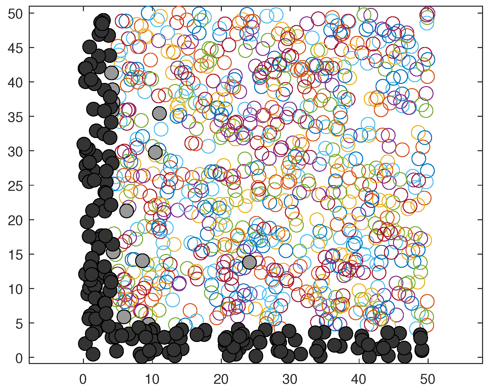
Example 2.

For this example, let $C:={\mathbb{R}}_{+}^2$, $⪯:={⪯}_C^{cert}$ and $H=\left\{{(1,1)}^T\right\}$. As the family of sets $\mathcal{A}$, we have randomly computed 1000 sets, for easy comparison each set is a ball of radius one in ${\mathbb{R}}^2$. We are interested in the $H^2$-approximate minimal elements of the set $\mathcal{A}$ and make use of Algorithm 2 to obtain those. Notice that Assumption 4 is trivially fulfilled. Out of the 1000 sets, a total number of 177 are $H^2$-approximate minimal w. r. t. to ⪯. Algorithm 2 generates at first 189 sets in $\mathcal{T}$; then, 177 sets are collected within the set $\mathcal{U}$ and $\mathcal{V}$. We used the same data as in Example 4.7 and 4.14 from [32], and according to our earlier results, a total number of 93 elements are minimal. In Figure 2, the sets within $\mathcal{T}$ are the lightly and darkly filled circles, while the $H^2$-approximate minimal elements of the set $\mathcal{A}$ (that is, the sets in $\mathcal{U}$ and $\mathcal{V}$) are the darkly filled circles. For comparison, Algorithm 2 is also used on the same family of sets with $H=\left\{{(0,0)}^T\right\}$ (see ([32], Example 4.7 and 4.14)), with 103 sets within $\mathcal{T}$ and 93 sets within $\mathcal{U}$ and $\mathcal{V}$, see Figure 3. Let us note that this example is chosen to illustrate the efficiency of Algorithm 2 as it is to be expected for problems with relatively homogeneous distribution of set size and structure, see the according discussion in the vector-valued case [15,43].

Of course, the notion of approximate minimality makes sense when minimal elements do not exist (in the vector-valued case, this can happen when the set of feasible elements in the objective space is open). In the future, we will study continuity notions of set-valued mappings that appear in set optimization problems and investigate existence results.

5. Conclusions

This paper investigates different kinds of approximate minimal solutions of set optimization problems. In particular, we present an inequality approach to characterize these approximate minimal solutions by means of a prominent scalarizing functional. To be as general as possible, our analysis is developed in real linear spaces without assuming any topology on the spaces and therefore bases only on algebraic relations and set inclusions between all the involved quantities. It would be interesting to study whether different scalarizing functionals may be used for a similar analysis as the separation functionals of Tammer–Weidner type have recently been embedded into a larger class of functionals [47]. We have proposed effective algorithms that select approximate minimal elements out of a family of finitely many sets. As a next step, it will be necessary to test our algorithms on practical examples.