Improving Initial Guess for the Iterative Solution of Linear Equation Systems in Incompressible Flow

Abstract

The pressure equation, generated while solving the incompressible Navier–Stokes equations with the segregated iterative algorithm such as PISO, produces a series of linear equation systems as the time step advances. In this paper, we target at accelerating the iterative solution of these linear systems by improving their initial guesses. We propose a weighted group extrapolation method to obtain a superior initial guess instead of a general one, the solution of the previous linear equation system. In this method, the previous solutions that are used to extrapolate the predicted solutions are carefully organized to address the oscillatory solution on each grid. The proposed method uses a weighted average of the predicted solutions as the new initial guess to avoid over extrapolating. Three numerical test results show that the proposed method can accelerate the iterative solution of most linear equation systems and reduce the simulation time up to 61.3%.

1. Introduction

The numerical simulation of incompressible flow is a complex nonlinear problem and governed by the Navier–Stokes equations [1,2,3]. There is vast literature for the numerical solution of the governing equations [4,5,6,7,8,9]. Among them, the segregated type algorithm, such as SIMPLE (Semi-Implicit Method for Pressure-Linked Equations) [10] and its variations [11,12], and PISO (Pressure Implicit with Splitting of Operator) [13], etc., are widely used in the commercial and open-source softwares, e.g., FLUENT [14] and OpenFOAM [15]. The segregated algorithm needs to solve the pressure equation generated in dealing with the pressure-velocity coupling. The implicit discretization schemes of the pressure equation usually lead to a series of linear equations in the form of

$$A^{k}x=b^k.$$

(1)

Here k is the index of the linear equation, $A^k$ and $b^k$ are the coefficient matrix and the right-hand-side, x is the primitive variable (e.g., the velocity, the pressure, etc.). Generally, the number of linear equation systems is quite large, resulting in a high computation cost. Therefore, it is essential to design efficient solution methods for these linear equation systems.

In real application simulations, the iterative methods, such as the Gauss-seidel method [16], Krylov methods [17], and multigrid methods [18,19,20], etc., are widely used for solving the linear equations [21]. In general, the iterative methods consist of four procedures: the construction of the preconditioner, the choice of the initial value, the computation of the next iterate, and the check for stopping criterion [22,23]. In the past decades, researchers are concerned about how to design an efficient and scalable preconditioner, see [24,25,26,27,28]. The choice of the initial guess is rarely studied because it has a close relationship with the applications, and it is not straightforward for the user to choose an optimal one.

In the last few decades, several methods were proposed for choosing a superior initial guess while solving a series of linear equation systems. These methods generally fall into two categories, namely the project-based method and the extrapolation-based method. The main idea of the projection-based method is first to construct a subspace, based on the information of previous linear systems, and then build a sub-linear system on this subspace and, at last, project the solution of the sub-linear system back to the original space as the improved initial guess. The various ways to construct the subspace induce several initial guess techniques. For linear equation systems with the same coefficient matrix and successive right-hand sides, Chan reused a set of direction vectors generated by solving previous linear systems with conjugate gradient (CG) method as the subspace [29]. He then calculated the approximate solutions by projecting the residual of other unsolved systems orthogonally onto the generated subspace. Fischer proposed an alternative way to construct the subspace for the same scene (linear systems with the same coefficient matrix but different right-hand-sides) in [30], where the subspace was built by Gram-Schmidt orthogonalization of the successive right-hand-side vectors. Later, in [31], Chan further extended his project method to solve multiple linear systems with different coefficient matrices. However, this method was still limited to be used in the CG method and hence, not applicable in other iterative methods, such as multigrid methods. In [23], the Krylov subspace produced by solving the previous linear equation system with GMRES was reused as the subspace. In [32], the Proper Orthogonal Decomposition (POD) method, based on some previous solutions, was used to construct the subspace. The induced initial guess method is applied in simulations of two-phase flow through heterogeneous porous media.

The other type of initial guess technique, extrapolation-based method, is seldom studied. The main idea of the extrapolation-based method is to calculate a better initial guess by the extrapolation techniques. In [22], a POD-based and a spectral-based extrapolation, based on previous solutions, are proposed for the spectral/hp element method. More recently, in [33], the Lagrange polynomial extrapolation based on previous solutions is used to calculate an approximation solution of the linear system. The approach is employed in SIMPLE-TS (semi-implicit method for pressure-linked equations-time step) finite volume iterative algorithm and applied to compressible Navier–Stokes–Fourier equations.

In the incompressible flow simulation, the initial guess of the current linear equation system is typically the solution of the previous one. However, while solving the pressure-velocity coupling, the solution on each cell usually appears to be oscillatory in successive linear equation systems, especially using some iterative algorithms such as PISO, etc. In this case, the previous solution is no longer an approximate solution for the current linear equation system. Also, the extrapolation method can hardly obtain a superior initial guess based on several previous solutions. One should handle the oscillatory solutions to avoid an inferior initial guess. In this paper, we propose a weighted group extrapolation method to improve the initial guesses for the series of linear equation systems in the incompressible flow. To address the oscillatory solutions, this method first partitions the linear equation systems into lanes and organizes some previous solutions in each lane into groups. After constructing the groups, we apply the extrapolation method in each group to predict the solution of the current linear equation system. The initial guess is then the weighted average of these predicted solutions. The contributions of this paper are summarized as follows:

• We propose a weighted group extrapolation method for improving the initial guess of the linear equation systems in incompressible flow.
• Some numerical tests are conducted to verify the effectiveness of the proposed method. Compared with the original method, the proposed method can reduce the solution time in most linear equation systems, and 61.3% of the cost can be saved at most.

The rest of the paper is organized as follows. In Section 2, we introduce the mathematic model of the incompressible flow and the numerical method of solving the pressure-velocity coupling. The motivation and details of the weighted group extrapolation method are present in Section 3. In Section 4, we report some numerical results. Finally, Section 5 is a summary of this paper.

2. Numerical Methods

The incompressible flow problem is governed by the Navier–Stokes equations, and therein the so-called pressure equation derived in the pressure-velocity coupling algorithm is the most time-consuming to be solved. In this paper, we concentrate on accelerating the iterative solution of the pressure equation. Here, the governing equations and the pressure-velocity coupling algorithm will be presented briefly in this section.

2.1. Governing Equations

Considering the unsteady incompressible flow in three-dimensions, the governing equations are

$$\begin{array}{c}\nabla ·U=0,\end{array}$$

(2)

$$\begin{array}{c}\frac{\partial U}{\partial t}+\nabla ·\left(UU\right)-\nabla ·((\nu +{\nu }_t)\nabla U)=-\nabla p,\end{array}$$

(3)

where $U=(u,v,w)$ and p are the relative velocity and relative pressure divided by the fluid density $\rho$ respectively; t is time, and $\nu$ here is the kinematic viscosity, ${\nu }_t$ is the turbulence viscosity which can be calculated by the turbulence model. Equations (2) and (3) are called the continuity equations and momentum equations, respectively. Please note that U and p are coupled in the momentum equations, which can be solved with the classical segregated algorithm such as SIMPLE and PISO. In general, these segregated algorithms work in a predictor-corrector manner. The predictor firstly guesses a value for p or sets p as a known value, such as the solution of the previous iteration. After predicting p, we can discretize and solve the momentum equations implicitly, and thus predict U. After the predictor, the predicted field U, together with the predicted field p, will satisfy the momentum equations. However, since p is inaccurate, the predicted field U obtained in this way usually does not satisfy the continuity equations. This question will be addressed by a corrector, where the so-called pressure equation is derived to correct U and p. The predictor-corrector works iteratively to drive U and p to satisfy the governing equations simultaneously. We will introduce the solution algorithm of the pressure-velocity coupling in the next subsection.

2.2. Solution Algorithm

The pressure-velocity coupling algorithm used in this paper is called PIMPLE [34], a combination of PISO and SIMPLE. The procedures of the predictor and corrector in PIMPLE are represented in the following part.

Without losing generality, we take the finite volume method (FVM) [3] as an instance to discretize the governing equations. In FVM, the computational domain is discretized into several control volumes. The discretization of the governing equations by integrating over a control volume e at time step n will yield algebraic equations of the form

$$\sum _{f\sim nb\left(e\right)}{S}_f{\mathbf{n}}_f·U_f^{n+1}=0,$$

(4)

and

$$a_e^{U^n}{U}_e^{n+1}+\sum _{v\sim nb\left(e\right)}{a}_v^{U^n}{U}_v^{n+1}=b_e^{U^n}-V_e{(\nabla p^{n+1})}_e,$$

(5)

where f represents the face around e and v represents the control volume surrounding e. $S_f$ is the area of f and ${\mathbf{n}}_f$ is the normal vector of f, and $V_e$ is the volume of the e. The coefficients $a_e^{U^n}$, $a_v^{U^n}$, and $b_e^{U^n}$ can be calculated explicitly, the superscript $U^n$ therein means that these coefficients depend on $U^n$. $U_f^{n+1}$ is the relative velocity on the face f, which can be calculated by Rhie-chow interpolation [35] using values in adjacent control volumes.

Denote the solution of the momentum equations in the predictor with a superscript *, that is, $U^{*}$ and $p^{*}$, then we have

$$\begin{array}{c}{a}_e^{U^n}{U}_e^{*}+\sum _{v\sim nb\left(e\right)}{a}_v^{U^n}{U}_v^{*}=b_e^{U^n}-V_e{(\nabla p^{*})}_e.\end{array}$$

(6)

Please note that $p^{*}$ is the solution of the previous iteration or time step. The algebraic Equation (6) of all control volumes then form the linear equation systems of $U^{*}$. We call the procedures of guessing $p^{*}$ and solving the linear equation system of $U^{*}$ the predictor. The predicted field $U^{*}$ and $p^{*}$ will not satisfy Equation (4), and they need further correction by the corrector. Since Equation (4) does not contain $p^{n+1}$ explicitly, we need to derive the so-called pressure equation to correct $U^{*}$ and $p^{*}$. Let $U^{**}$ and $p^{**}$ denote the fields after the corrector, and they satisfy Equation (5). Since $U^{*}$ is already known, it can be used to estimate the second term of Equation (5). Thus $U_e^{**}$ can be expressed as

$$U_e^{**}=-\sum _{v\sim nb\left(e\right)}\frac{a_v^{U^n}}{a_e^{U^n}}{U}_v^{*}+b_e^{U^n}-V_e{(\nabla p^{**})}_e.$$

(7)

By combining Equations (4) and (7) on all the control volumes, the linear equation system of $p^{n+1}$ can be derived as

$$A^{U^n}{p}^{**}=b^{U^{*}},$$

(8)

where $A^{U^n}$ is the coefficient matrix that depends on $U^n$, and $b^{U^{*}}$ is the right-hand-side that depends on $U^{*}$. We call Equation (8) the pressure equation. After Equation (8) is solved, $U^{**}$ on each control volume can be obtained by Equation (7). We call the procedure of solving the linear equation system of $p^{**}$ and correcting $U^{**}$ the corrector.

Please note that both the predictor and corrector can be applied many times as desired in PIMPLE. The flowchart in Figure 1 can describe the main procedure of PIMPLE [34].

We also show where our method should be used in this figure. Please note that in Figure 1, the loop limits of pimplpe.loop and pimple.correct, denoted by L and C respectively, are two prescribed numbers. When L is 1, this algorithm is the PISO algorithm.

The number of linear equation systems for U and p needed to solve within a single time step is $3L$ (L for each component of U) and $LC$, respectively. The number of linear equation systems increases rapidly as the number of time step increases, and the overhead it takes to solve these linear equation systems will be very high. Therefore, an efficient iterative solution method for these linear equations is essential for the simulation.

3. The Weighted Group Extrapolation Method

Initial guess has a critical impact on the iterative solution efficiency of the linear equation system. In this section, we first present our motivation by discussing the influence of the initial guess. Then, we provide an instance to illustrate the disadvantage of the current initial guess, followed by our method in detail.

3.1. Motivation

For the linear equation system

$$Ax=b$$

(9)

with the initial guess $x_0$, the convergence criterion for an iterative method is generally

$$\frac{\parallel b-A{x}_k{\parallel }_2}{{\parallel b\parallel }_2}<ϵ,$$

(10)

or

$$\frac{\parallel b-A{x}_k{\parallel }_2}{\parallel b-A{x}_0{\parallel }_2}<ϵ,$$

(11)

where k is the iteration number, $ϵ$ is a user-defined value. The left-hand side of Equations (10) and (11) are the so-called absolute residual and relative residual, respectively.

The convergence criterion is quite critical since it determines the effectiveness of the initial guess. In particular, if the convergence criterion is Equation (10), it may need fewer iterations to converge the linear equation system when the initial guess is closer to the solution. For instance, if the accurate solution is set as the initial guess, Equation (10) will be satisfied immediately, and no iteration is needed. Conversely, if the convergence criterion is Equation (11), it still requires iterations even if the initial guess is very close to the accurate solution. Fortunately, in most simulations, Equation (10) is a common choice; thus, if one can obtain the initial guess that is closer to the solution, it is possible to reduce the iteration number and earn a speedup in terms of solution time.

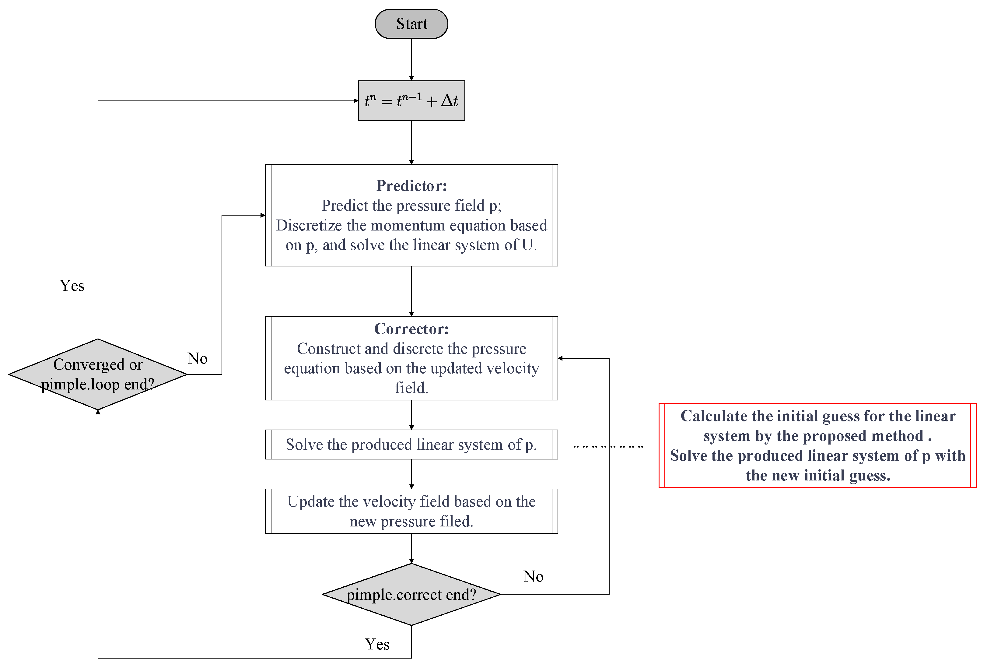
In the simulation of incompressible flow, when applying PIMPLE to solve the pressure-velocity coupling, the updating trace of the fields from the nth time step to $(n+1)$th time step is drawn as Figure 2.

As the time step advances, a series of linear equation systems of $p^{**}$ in the form of Equation (1) arises when solving the pressure equations. Moreover, the initial guess of the current linear equation system is usually the solution of the previous one (i.e., the solution of the previous corrector). In the PIMPLE algorithm, the predictor-corrector will drive the fields $p^n$ and $U^n$ to converge to the final solutions $p^{n+1}$ and $U^{n+1}$. 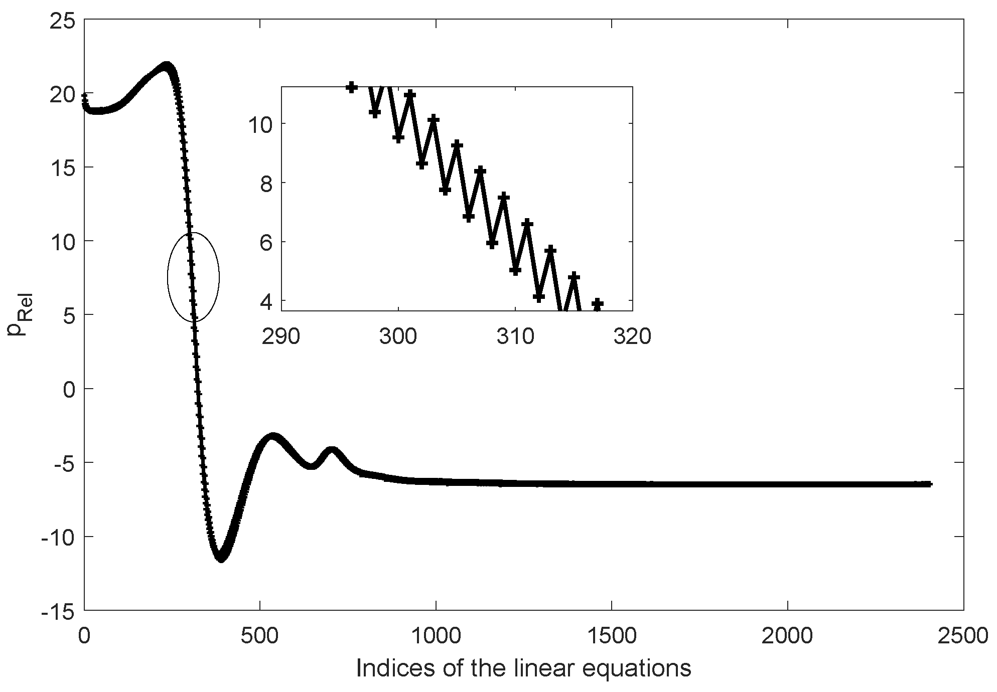However, since the predicted fields $p^{*}$ and $U^{*}$ are inaccurate, it is easy for the corrector to overcorrect the fields such that the convergence history of the fields on each cell may be oscillatory. To illustrate the oscillatory situation more clearly, we record how $p^{**}$ changes along with the indices of the linear equations on one probe cell in a tutorial case (called pitzDaily in OpenFOAM). The history of $p^{**}$ on the probe cell is shown in Figure 3. Please note that in this case, L is 1 and C is 2, i.e., in each PIMPLE iteration, a predictor followed by two correctors are used to solve the coupling systems. Also, note that $p^{**}$ here is defined as

$$p_{Rel}=p-\frac{p_{Ref}}{\rho },$$

(12)

where $p_{Ref}$ is the reference pressure, $\rho$ is the density, and p is the relative pressure.

From Figure 3, one can see that the field on the probe cell is oscillatory in successive linear equations. Under this circumstance, the solution of the previous linear equation will be far away from the solution of the current one, and it is no longer an appropriate initial guess. This indicates that we should take the initial guess of the linear equation into further consideration.

3.2. The Weighted Group Extrapolation Method

To address the inferior initial guess caused by the oscillatory solutions, we partition all the linear equation systems into several lanes. Each lane is a set of linear equation systems, and the history of solutions on each cell are expected to be “smooth” in each lane. More precisely, given the sequence of linear equations in the form of Equation (1), the ith lane is defined as

$$\begin{array}{c}\mathcal{L}\left(i\right)=\left\{A^{k}x=b^k,k=i+tN\right\},\\ i=0,\cdots ,N-1,\end{array}$$

(13)

where t is the time step, and N is the total number of the lanes. In the PIMPLE algorithm, N equals the number of correctors in each time step, i.e., $N=LC$. After defining the lane, we can describe the weighted group extrapolation method in detail.

The main idea of our method is to calculate the initial guess of the linear equation system based upon some previous solutions in the same lane. We use a fixed size window to constrain the number of previous solutions that need to be stored, and calculate the initial guess based on the solutions within this window. The window size, say W, is predefined by the user to limit the storage overhead introduced by our method. Let ${\mathcal{S}}_l^m$ be the set of solutions in the window that will be used to calculate the initial guess of the mth linear equation in $\mathcal{L}\left(l\right)$. It can be described by

$${\mathcal{S}}_l^m=\left\{x_l^k,k\in [m-W,m-1]\right\},$$

(14)

where $x_l^k$ is the solution of the kth linear equation system in $\mathcal{L}\left(l\right)$. Now we can present our weighted group extrapolation method by the following steps.

(1)

Construct the groups. We partition the set ${\mathcal{S}}_l^m$ into G groups, and each group consists of $W/G$ elements. Moreover, the indices of the elements in each group should have the same differences. That is,

$${\mathcal{S}}_l^m=\bigcup {\mathcal{G}}_l^i,i=0,\cdots ,G-1,$$

(15)

where ${\mathcal{G}}_l^i$ is constructed by

$$\begin{array}{c}{\mathcal{G}}_l^i=\left\{x_l^k,k=m-W+i+nG\right\}\\ n=0,\cdots ,\frac{W}{G}-1.\end{array}$$

(16)

To keep the size of each group the same, the window size W should be the integral multiple of the number of the groups.

(2)

Predict the solution in each group. Once the groups are constructed, each group will predict a solution using a specific extrapolation method. Let ${\mathtt{x}}_l^i$ be the solution predicted by the ith group, then we have

$${\mathtt{x}}_l^i=\mathbf{EXTP}\left({\mathcal{G}}_l^i\right).$$

(17)

Here $\mathbf{EXTP}$ represents the extrapolation method such as Lagrange’s polynomial, cubic splines, etc. [36]. The extrapolation method uses the indices of the previous solutions in the windows as the positions of the extrapolated points. We use a simple instance to illustrate how this step works in the following part.

(3)

Sum the weighted predictions up. After each group obtains the predicted solution, the initial guess is determined by

$$x_l^0=\sum _{i=0}^{G-1}{w}_l^i{\mathtt{x}}_l^i,$$

(18)

where $w_l^i$ is the weight of the ith group, and it is an empirical parameter and is predefined by users.

Example 1.

To describe the proposed method more clearly, we use a simple example to demonstrate the procedure of our method. Consider the following set of linear equation systems

$$\{L_i:A_i{x}_i=b_i,i=0,1,\cdots ,9\}.$$

Suppose the linear systems $L_0\sim L_7$ were solved already, and $\underline{x_0}\sim \underline{x_7}$ are the corresponding solutions. Suppose the number of correctors in each time step in the PIMPLE algorithm is 2, i.e., $N=2$. Now our method calculates the initial guesses for $L_8$ and $L_9$ in the following way.

(1) 

At the beginning of our method, we select the previous solutions that are used to extrapolate the initial guesses carefully, according to the specific setting of the PIMPLE algorithm. This procedure is critical for our method. Since $N=2$, we partition all the linear systems into two lanes, namely

$$\mathcal{L}\left(0\right)=\{A_i{x}_i=b_i,i=0,2,4,6,8\},$$

(19)

and

$$\mathcal{L}\left(1\right)=\{A_i{x}_i=b_i,i=1,3,5,7,9\}.$$

(20)

Now, there are five linear equation systems in each lane, and our method will calculate the initial guesses for $L_8$ and $L_9$ using the known solutions in each lane. If we set the size of the window size to 4 ($W=4$), then the solutions that are used to calculate the initial guesses of the 5th linear systems in each lane, i.e., ${\mathcal{S}}^5$, is obtained straightforwardly as

$${\mathcal{S}}_0^5=\left\{\underline{x_0},\underline{x_2},\underline{x_4},\underline{x_6}\right\},$$

(21)

and

$${\mathcal{S}}_1^5=\left\{\underline{x_1},\underline{x_3},\underline{x_5},\underline{x_7}\right\}.$$

(22)

If we use a linear extrapolation method in the following steps, we can partition ${\mathcal{S}}^5$ into two groups, that is,

$${\mathcal{S}}_0^5=\left\{\underline{x_0},\underline{x_4}\}\cup \{\underline{x_2},\underline{x_6}\right\},{\mathcal{G}}_0^0=\{\underline{x_0},\underline{x_4}\},{\mathcal{G}}_0^1=\{\underline{x_2},\underline{x_6}\},$$

(23)

and

$${\mathcal{S}}_1^5=\left\{\underline{x_1},\underline{x_5}\}\cup \{\underline{x_3},\underline{x_7}\right\},{\mathcal{G}}_1^0=\{\underline{x_1},\underline{x_5}\},{\mathcal{G}}_1^1=\{\underline{x_3},\underline{x_7}\}.$$

(24)

(2) 

After constructing the groups, we can now predict the solution in each group. Here we use the linear Lagrange function to predict the solution within each group. For example, we use two points, $(1,\underline{x_0})$ and $(3,\underline{x_4})$, to compute the predicted solution in ${\mathcal{G}}_0^0$. That is,

$${\mathtt{x}}_0^0=\frac{5-1}{3-1}\underline{x_0}+\frac{5-3}{1-3}\underline{x_4}.$$

(25)

Here 1, 3, and 5 are the positions of the corresponding solutions in the window. Similarly, we can compute the predicted solutions, ${\mathtt{x}}_0^1$, in the second group, and also ${\mathtt{x}}_1^0$ and ${\mathtt{x}}_1^1$ in the second lane.

(3) 

Once each group gets its predicted solution, we calculate the final initial guesses for $L_8$ and $L_9$ by

$$x_0^0=\frac{{\mathtt{x}}_0^0+{\mathtt{x}}_0^1}{2}$$

(26)

and

$$x_1^0=\frac{{\mathtt{x}}_1^0+{\mathtt{x}}_1^1}{2},$$

(27)

respectively. Here the weight of each group is 0.5.

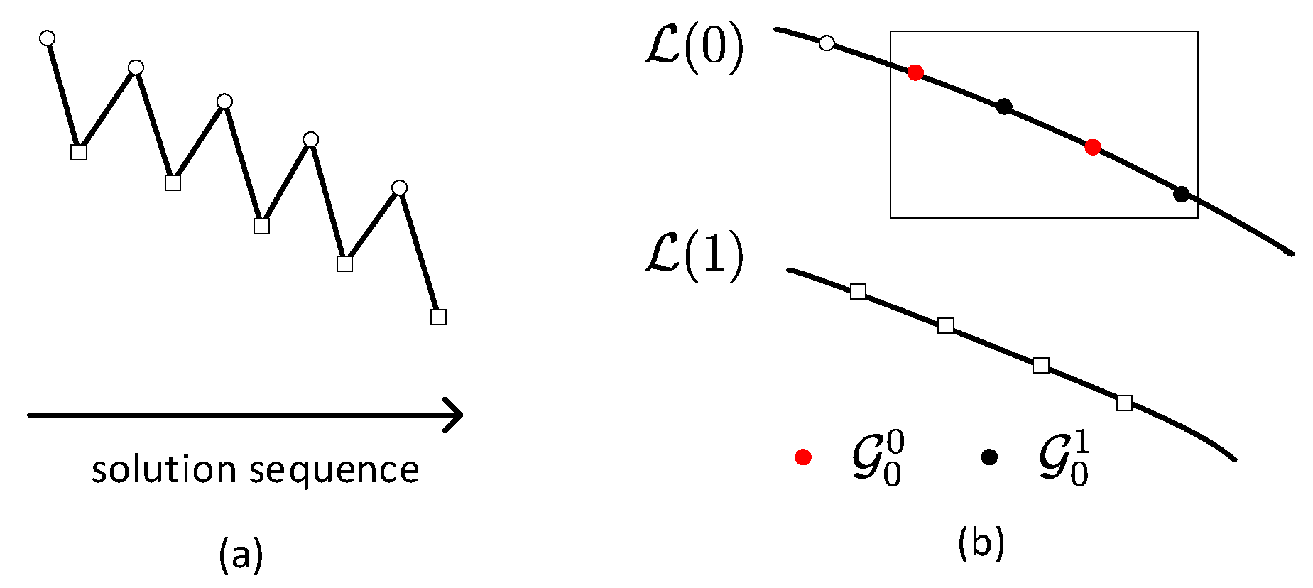
Figure 4 is a simple illustration of the construction of the groups in our method. Figure 4a represents the sequence of the solution as the time step advances, the circle represents the solution from the first corrector, and the square represents the solution from the second corrector. The linear equation systems from the first and the second corrector will form $\mathcal{L}\left(0\right)$ and $\mathcal{L}\left(1\right)$, respectively. Each line in Figure 4b represents a lane. In $\mathcal{L}\left(0\right)$, we use different colors to mark the solutions that belong to different groups.

The weighted group extrapolation method will introduce extra computational and storage overhead compared with the original method. If we want to improve the initial guesses in all the lanes, the additional storage overhead will be $N\times W$ times of the solution vector. It may cause a loss of performance when N and W enlarge. To avoid an expensive storage cost, one can constrain the window size W. On the other hand, instead of improving the initial guess in all lanes, one can apply the method in some selected lanes. Moreover, one can use the method within some selected time steps.

Please note that the proposed method is in a general form. The group size and the extrapolation method are adjustable in our method, and they must keep consistent with each other. For instance, a group that consists of two elements can only use a linear method to extrapolate the predicted value. If one wants to use the polynomial method in higher-order, the size of the group should be larger. The weight of each group provides a way for the user to adjust the relaxation on the predicted values. In this way, the method avoids the lousy prediction caused by the singular one. In this paper, the choice of the extrapolation method, as well as the weight for each group, is simplified. To be specific, we use a linear extrapolation method in our method, and the weight for each group is 0.5.

4. Numerical Result

To test the effectiveness of the weighted group extrapolation method, three cases are conducted in this section. One is the tutorial case called pitzDaily in OpenFOAM. The other two cases are a tow-dimensional (2D) NACA0012 airfoil and a three-dimensional (3D) blended-wing-body airfoil from Li C. et al. [37].

The weighted group extrapolation method is implemented and tested in the platform of OpenFOAM (version 4.0) [15], which uses the finite volume method to discretize the governing equations. We solve all these three cases by the application called pimpleFoam, which is a solver for incompressible unsteady flow in OpenFOAM [38]. It uses the PIMPLE algorithm to solve the pressure-velocity coupling. In this test, the weighted group extrapolation method is only used to improve the initial guess of the linear equation systems arising from the pressure equations, which is the central time overhead. In each linear equation system, the iterative method is the geometric algebraic multigrid (GAMG) [39] method (the default method for the pressure field in the case of OpenFOAM). The smoother used here is the DIC-Gauss-Seidel, which is the combination of diagonal incomplete-Cholesky and Gauss-Seidel. The other parameters of GAMG are default in OpenFOAM.

We compare the performance of the weighted group extrapolation method with the default method in OpenFOAM. In the weighted group extrapolation method, the window size W is set to 4, and the group number G is set to 2. Consequently, the group size is 2, and the linear method is used to predict the solution in each group. The weight of each group is 0.5. All experiments are conducted on an E5-2620 CPU with 2.10 GHz and a RAM of 64GB. E5-2620 has a total of 12 cores on two sockets. We run the pitzDaily case in sequence, and run the 2D and 3D airfoil cases in parallel.

To present the results, we use the following notations to represent the specific methods:

• GAMG: The GAMG method with the default initial guess in OpenFOAM.
• GAMG-WGE: The GAMG method with the initial guess obtained by the weighted group extrapolation method.

Furthermore, the following notations are used to report the results.

• $T_n\mathcal{L}\left(m\right)$: The linear equation system in the mth lane at the nth time step.
• $Ncell$: The number of mesh cells or the scale of the linear equation system.
• $Nprocs$: The number of processors used in the simulation.
• $Nit$: The iteration number of the iterative method for solving a linear equation system.
• $Nits$: The total iteration number for solving all the linear equation systems arising from the pressure equations.
• $R_{init}$: The initial residual of the linear equation system.
• $T^p\left(s\right)$: Total time for solving a single linear equation system arising from the pressure equation in seconds.
• $T_{total}^p\left(s\right)$: Total time for solving all the linear equation systems arising from the pressure equations in seconds.
• $T_{total}\left(s\right)$: Total time for the whole simulation in seconds.
• $S_p$: The speedup of the total time for solving the linear equation system by the GAMG-WGE method compared with the GAMG method.
• $S_{total}$: The speedup of the total time for the simulation with the GAMG-WGE method compared with the GAMG method.

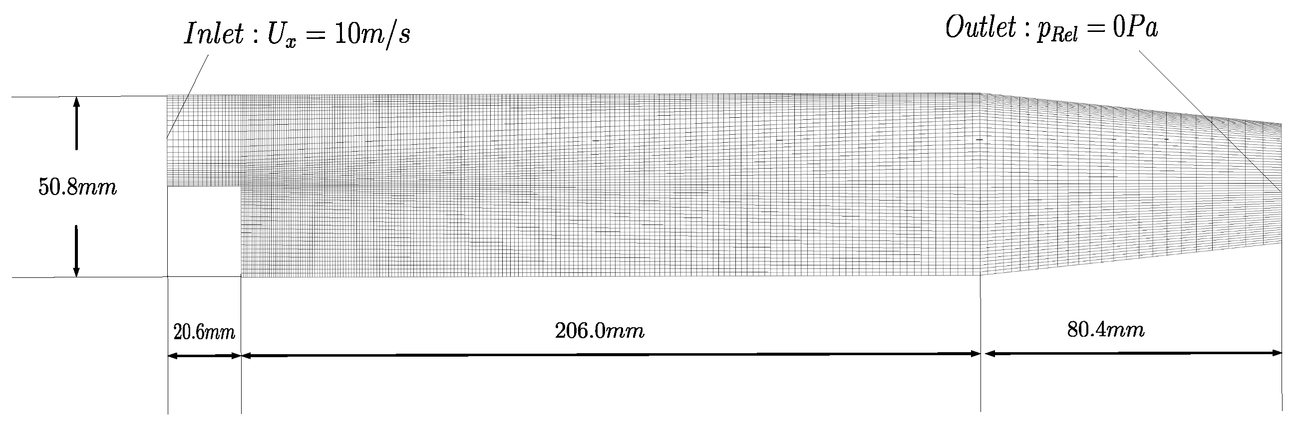
4.1. PitzDaily

PitzDaily is a case that simulates the fluid flowing over a backward-facing step. It is the tutorial case for the solver pimpleFoam in OpenFOAM. The turbulence model used is the k-$ϵ$ model. The numerical schemes for the discretization are default in OpenFOAM. Figure 5 shows the basic mesh in this case, and its cell number counts 12,225 totally.

In this case, L and C are 1 (by default) and 2 (by default), respectively. In fact, this setting of PIMPLE will act as the PISO algorithm. With this setting, the number of linear equation systems arising from the pressure equations is 2, as is the number of lanes in the GAMG-WGE method. The tolerance in OpenFOAM is ${10}^{-4}$ for the linear equation system in $\mathcal{L}\left(0\right)$ and ${10}^{-7}$ for the linear equation system in $\mathcal{L}\left(1\right)$, respectively. We simulate from $0s$ to $0.3s$, and the time step size is adjustable and limited by the allowed max courant number, which is set to 5 here.

To study the effect of the GAMG-WGE method, we extract the linear equation systems in $\mathcal{L}\left(1\right)$ at 50th, 100th, 200th, 500th, and 1000th time steps from the simulation.

Table 1. Test result of some linear equation systems in pitzDaily ${}^{†}$.

$\mathit{T}\#\mathcal{L}\left(1\right)$	Method	${\mathit{R}}_{\mathit{init}}$	$\mathit{Nit}$	${\mathit{T}}^{\mathit{p}}$	${\mathit{S}}_{\mathit{p}}$
T50	GAMG	$6.2\times {10}^{-2}$	18	0.044	-
	GAMG-WGE	$1.8\times {10}^{-2}$	14	0.034	1.27
T100	GAMG	$3.4\times {10}^{-2}$	15	0.036	-
	GAMG-WGE	$1.0\times {10}^{-2}$	11	0.027	1.33
T200	GAMG	$2.7\times {10}^{-2}$	20	0.049	-
	GAMG-WGE	$1.1\times {10}^{-2}$	13	0.032	1.50
T500	GAMG	$6.9\times {10}^{-4}$	11	0.027	-
	GAMG-WGE	$2.0\times {10}^{-3}$	11	0.028	0.97
T1000	GAMG	$2.9\times {10}^{-4}$	9	0.022	-
	GAMG-WGE	$2.0\times {10}^{-3}$	9	0.023	0.97

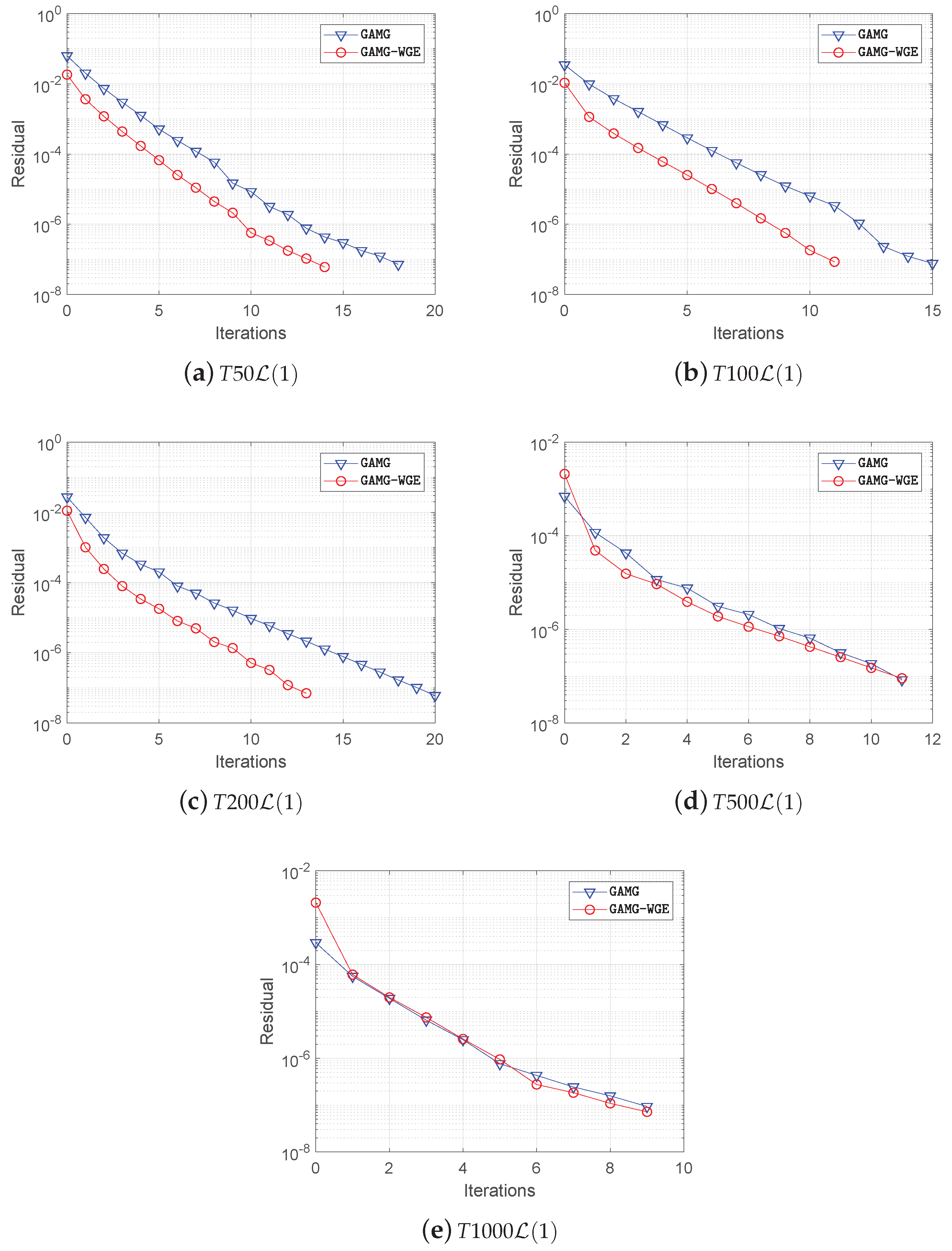
${}^{†}$$Ncell=12,225,Nprocs=1$.

is the test result of these linear equation systems. From Table 1, one can see that the GAMG-WGE method leads to a lower initial residual than the GAMG method in the case at 50th, 100th, and 200th time steps. As a result, the iteration numbers, as well as the solution time in these cases are smaller. Therefore, the GAMG-WGE method manages to achieve $1.27$×, $1.33$×, and $1.50$× speedups in these cases, respectively. Additionally, the GAMG-WGE method fails in the case at 500th and 1000th time steps, where the initial residuals solved by GAMG-WGE are larger compared with GAMG. Although the iteration number remains the same, the GAMG-WGE has introduced some additional computations. Therefore, there is a loss in the performance by using the GAMG-WGE method in these two linear equation systems. Figure 6 records the convergence history of the residual of the extracted linear equation systems. The effect of the GAMG-WGE method on the convergence can be seen clearly from this figure.

Before investigating the effectiveness of our method for the full simulation, we use a projection method-based solver as the reference to verify the correctness of our method. The projection method-based solver denoted as RK4-PM in the following part is a fourth-order Runge–Kutta projection method based on the Chorin–Temam algorithm [40,41]. One can find the details of the implementation of the projection method in Vuorinen’s paper [42]. 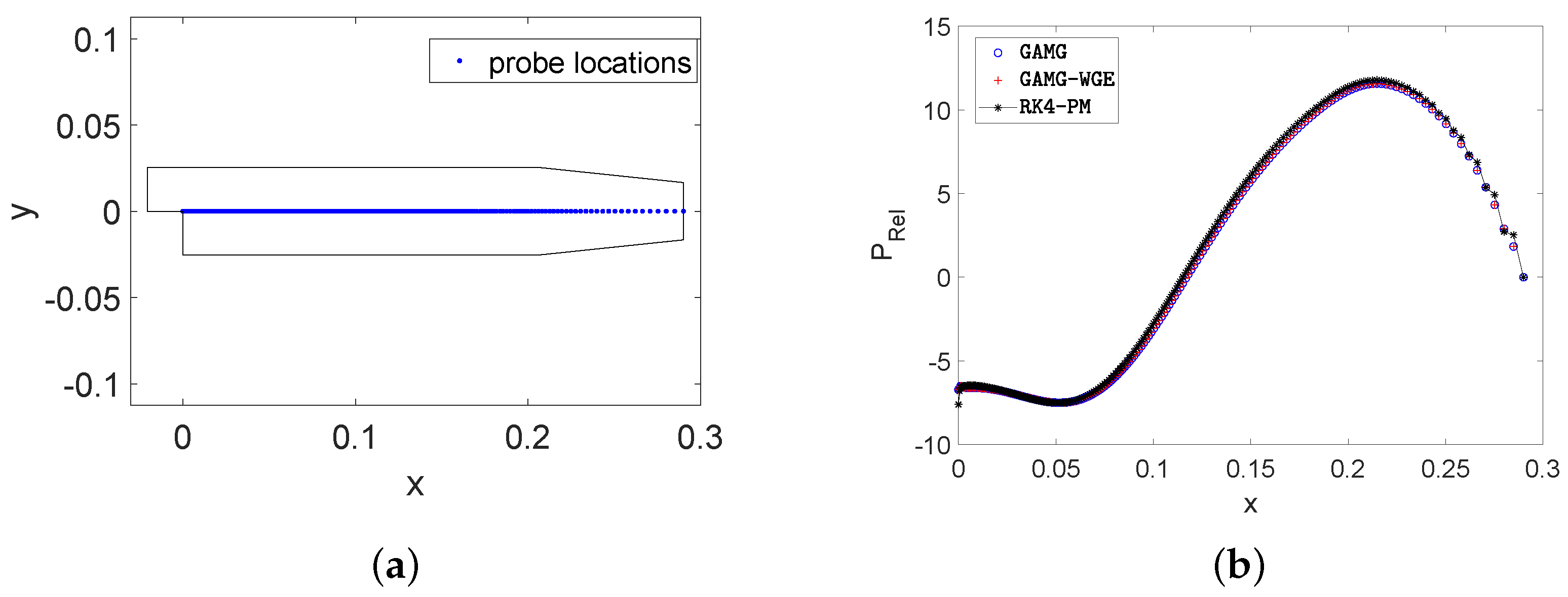Figure 7 compares the $p_{Rel}$ field at 0.3s obtained by each method. It shows that the distributions of the $p_{Rel}$ fields of these methods are almost the same. Moreover, Figure 8 compares the $p_{Rel}$ values at specific probe locations (i.e., the line located in the middle of the computational domain along the x-axis), and it also shows a consistent result.

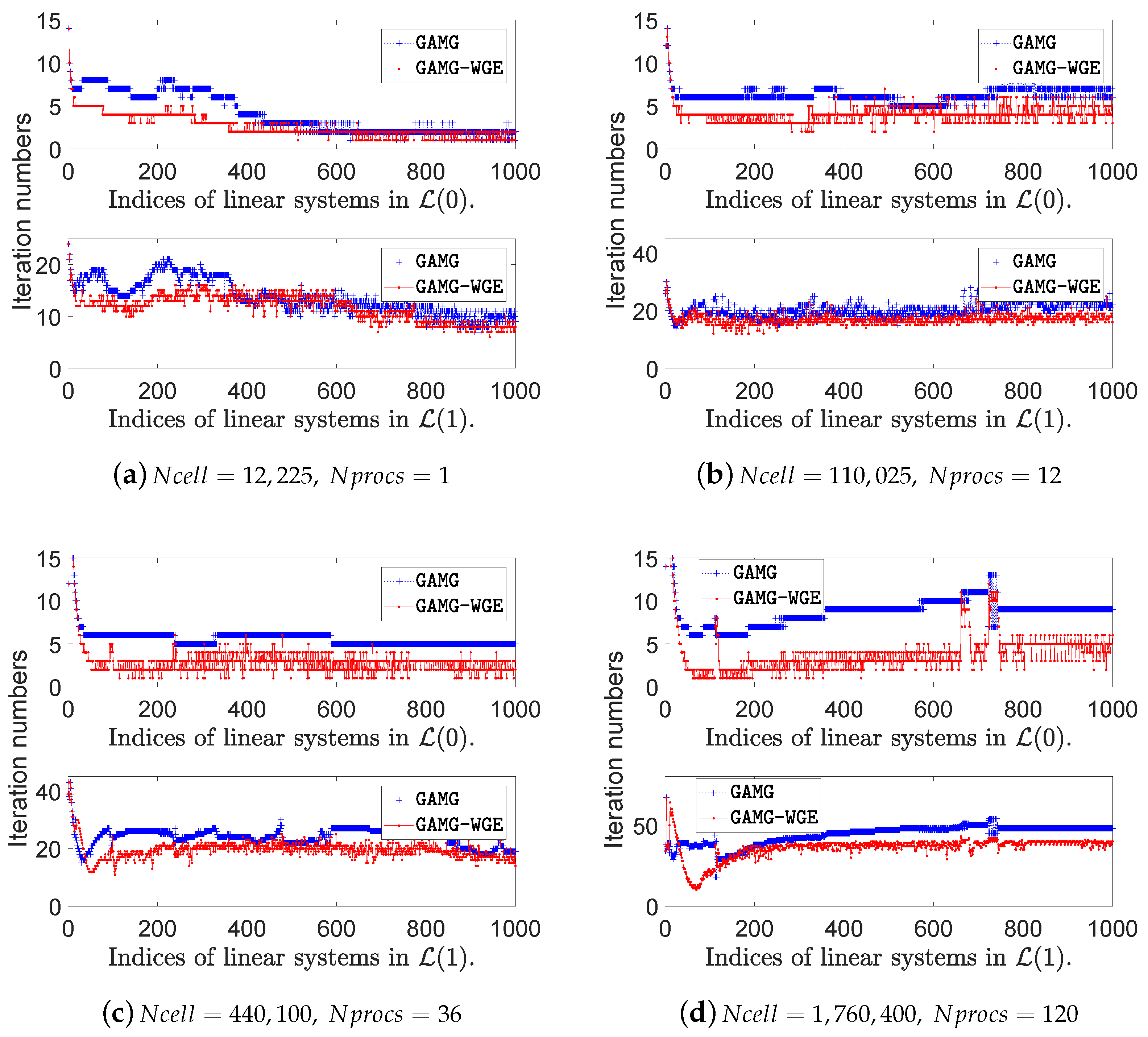
To show the effectiveness of the proposed method, we run this case in several mesh scales. We keep around ten-thousands cells on each processor. When the mesh scale is large, we partition the mesh into several sub-domains by the decomposePar application in OpenFOAM using the scotch approach and run the solver in parallel. Figure 9 shows the comparisons of the iteration number of each linear equation system in the first 1000 time steps with and without our method.

Please note that in this case, we begin to apply the GAMG-WGE method from the 10th time step. The result in Figure 9 has shown that the GAMG-WGE method leads to a lower iteration number than the GAMG method in most linear equations, in all the mesh scales. As a result, the total iteration number for the linear equation systems in the pressure equations is reduced by using the GAMG-WGE method, as is reported in

Table 2. The test result of pitzDaily.

$\mathit{Ncell}$	$\mathit{Nprocs}$	Method	$\mathit{Nits}$	${\mathit{T}}_{\mathit{total}}^{\mathit{p}}$	${\mathit{T}}_{\mathit{total}}$	${\mathit{S}}_{\mathit{p}}$	${\mathit{S}}_{\mathit{total}}$
12,225	1	GAMG	17,827	44.4	75.5	-	-
		GAMG-WGE	14,439	37.0	67.9	1.20	1.11
110,025	12	GAMG	26,522	79.8	120.2	-	-
		GAMG-WGE	21,048	64.8	105.1	1.23	1.14
440,100	36	GAMG	29,662	197.4	250.1	-	-
		GAMG-WGE	22,464	152.1	205.1	1.30	1.22
1,760,400	120	GAMG	52,888	664.0	763.4	-	-
		GAMG-WGE	39,967	514.7	614.0	1.29	1.24

. Further, the solution time for all the linear equation systems of the pressure equations, as well as the total simulation time, is reduced.

As is listed in Table 2, the speedup of solution time for the pressure equation is about $1.20$× to $1.30$× in all the mesh cases, and the associated speedup of the overall simulation time is about $1.1$× to $1.24$×. Furthermore, one can see that as the cell number grows, the linear systems produced by the pressure equation need more iterations to converge, which can also be seen in Figure 9. As a consequence, the solution time of the pressure equations takes up more time in the whole simulation. Thus, the proposed method is more effective when the pressure equations are more time-consuming in the simulation.

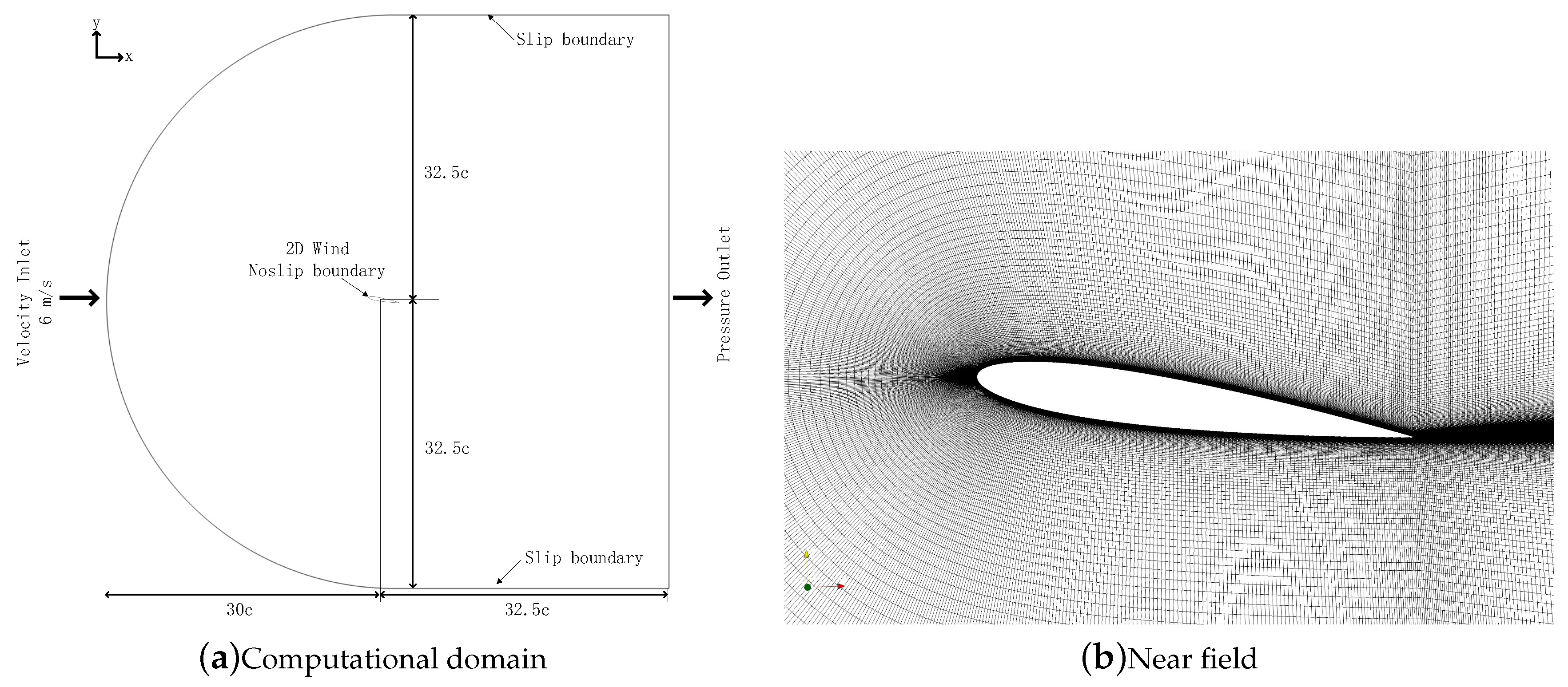
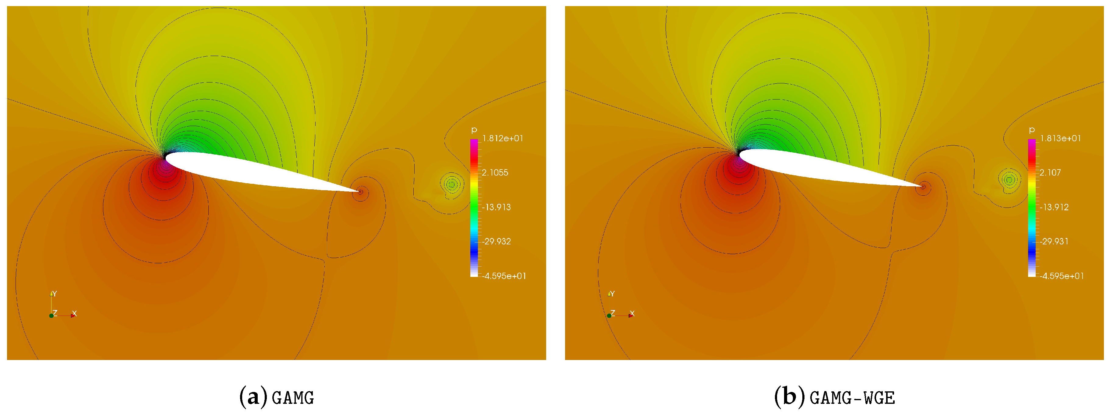
4.2. 2D NACA0012

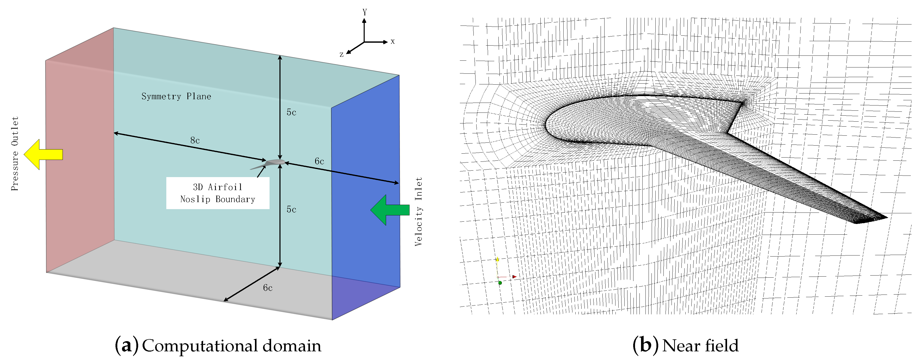
This case simulates the water flowing over a two-dimensional (2D) NACA0012 airfoil. The chord of airfoil c is 1 m, so the Reynolds number based on the chord is $6E6$. The angle of attack is ${10}^{\circ }$. Figure 10 shows the mesh, including the whole flow field and the near field of the airfoil. The number of cells is 165,392. Before running, the computational mesh is decomposed to 12 sub-domains by the decomposePar application in OpenFOAM using scotch. Twelve processors are used to simulate from 0 s to 0.1 s. The time step is adjustable and limited by the allowed max courant number, which is set to 5 here.

In this case, both L and C are 2. Please note that in each corrector of PIMPLE, two additional pressure equations will be solved to deal with non-orthogonal meshes. Thus, the number of lanes, in this case, is 8, i.e., $N=8$. The tolerance in OpenFOAM is ${10}^{-8}$ for the linear equation system in $\mathcal{L}\left(3\right)$ and $\mathcal{L}\left(7\right)$, and ${10}^{-4}$ for the rest. In this test, the GAMG-WGE method is only applied in $\mathcal{L}\left(3\right)$ and $\mathcal{L}\left(7\right)$, and it starts after 10 time steps.

To verify the correctness of our method, we compare the distribution and contour of the $p_{Rel}$ field and the specific values of $p_{rel}$ at some probes at 0.1s obtained by different methods, which are shown in Figure 11 and Figure 12 respectively. Moreover, we provide the absolute summation of continuity errors in all cell volumes along with the time steps in Figure 12 to further illustrate the consistent results obtained by different methods.

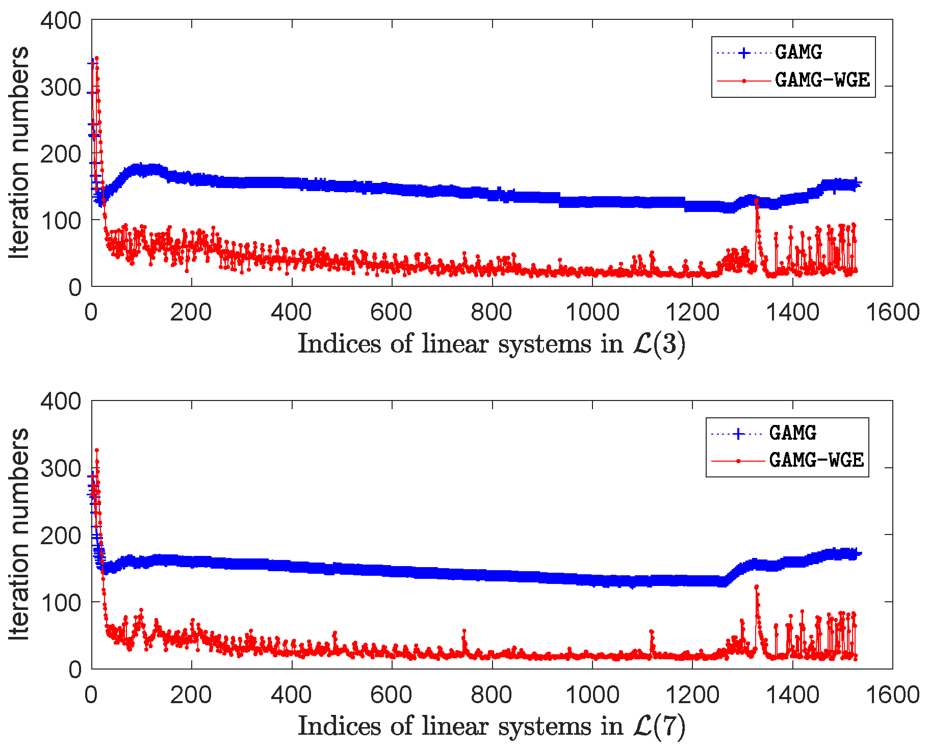
Moreover, Figure 13 records the iteration number of each linear equation system in $\mathcal{L}\left(3\right)$ and $\mathcal{L}\left(7\right)$ solved by different methods. It is clear that in both lanes, the GAMG-WGE method requires much lower iteration numbers than the GAMG method in most linear equation systems. We report the result of the total iteration number and solution time in

Table 3. The test result of 2D NACA0012 airfoil ${}^{†}$.

Method	$\mathit{Nits}$	${\mathit{T}}_{\mathit{total}}^{\mathit{p}}$	${\mathit{T}}_{\mathit{total}}$	${\mathit{S}}_{\mathit{p}}$	${\mathit{S}}_{\mathit{total}}$
GAMG	498,679	3166.9	3404.0	-	-
GAMG-WGE	165,532	1078.4	1317.0	2.93	2.58

${}^{†}$$Ncell=165,392,Nprocs=12$.

. From Table 3, one can see that the total iteration number of all the linear equation systems is reduced by $66.8\%$ using the GAMG-WGE method. Consequently, the total solution time of the pressure equations is reduced by $65.9\%$, and the total simulation time is reduced by $61.3\%$.

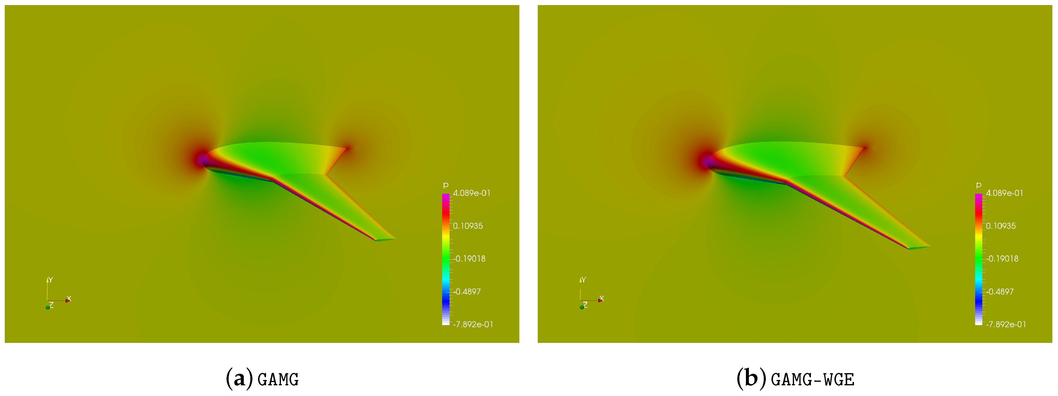
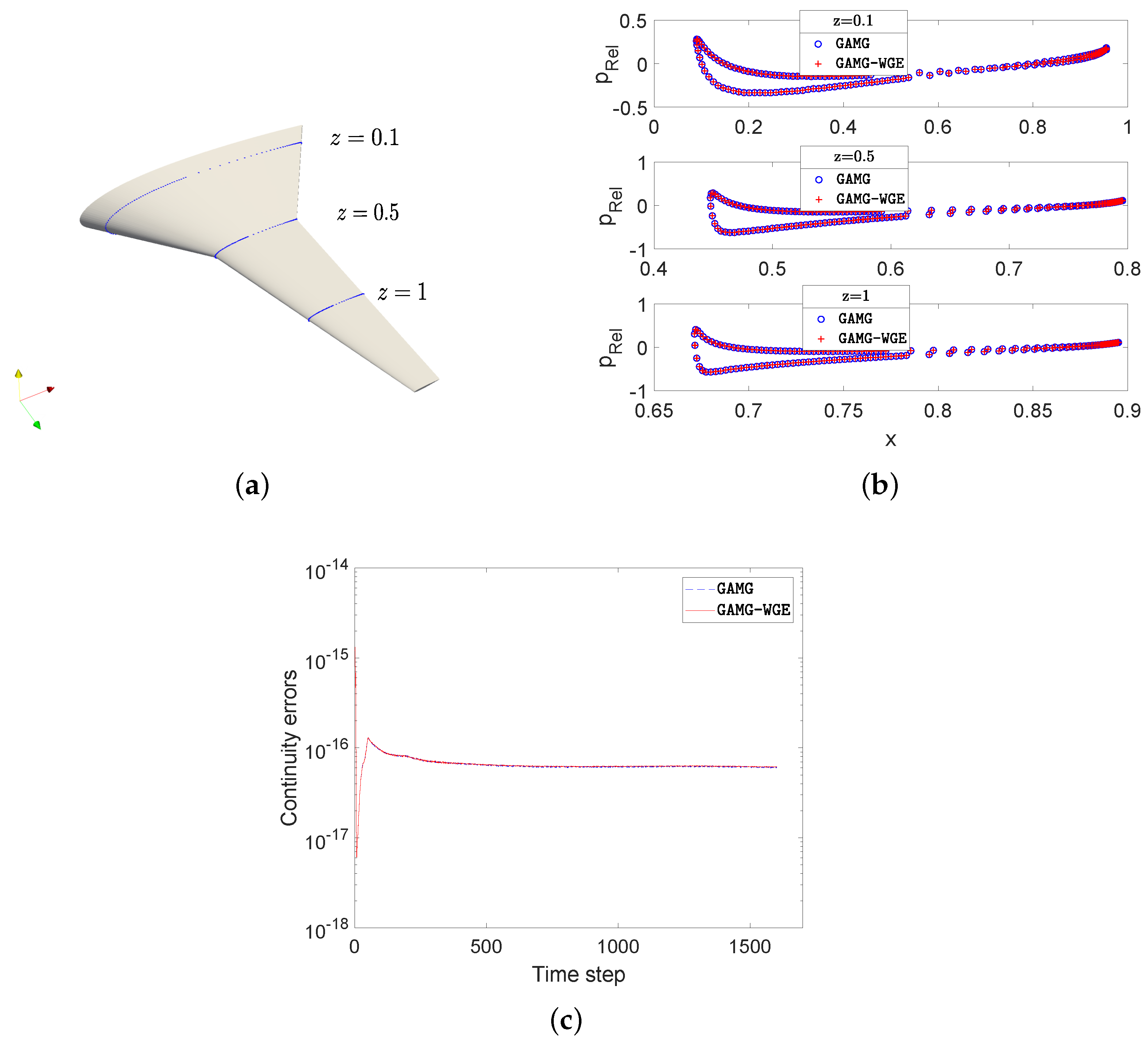
4.3. 3D Blended-Wing-Body Airfoil

In this subsection, the performance of the GAMG-WGE method in the case of three-dimensional (3D) blended-wing-body airfoil is tested. This case verifies the effectiveness of our method in the 3D application with a large number of processors. The chord of airfoil c is 1 m, so the Reynolds number based on the chord is $1E6$. The angle of attack is $6^{\circ }$.

The mesh is shown in Figure 14, including the far-field boundary and the near field of the airfoil. The number of cells is 4,255,146. Also, this simulation runs in parallel. The computational mesh is decomposed to 240 sub-domains by the decomposePar in OpenFOAM using scotch. The number of processors used here is 240. We simulate the case from 0 s to 0.1 s. The time step is adjustable and limited by the allowed max courant number, which is set to 5 here.

The settings of the PIMPLE algorithm are the same within the 2D NACA0012 case, that is, $L=2$ and $C=2$. Also, two additional pressure equations will be solved to deal with non-orthogonal meshes, and the number of lanes is 8. The tolerance in OpenFOAM is ${10}^{-8}$ for the linear equation system in $\mathcal{L}\left(3\right)$ and $\mathcal{L}\left(7\right)$, and ${10}^{-4}$ for the rest. In this test, the GAMG-WGE method is only used in $\mathcal{L}\left(3\right)$ and $\mathcal{L}\left(7\right)$, and it starts after 10 time steps.

Figure 15 and Figure 16 are provided to verify the correctness of our method. We compare the distribution of the $p_{Rel}$ field and the specific values on some probes at 0.1 s obtained by different methods. The figures show that the results are consistent. Moreover, we provide the absolute summation of continuity errors in all cell volumes along with the time steps in Figure 16 to further illustrate the consistent results obtained by different methods. 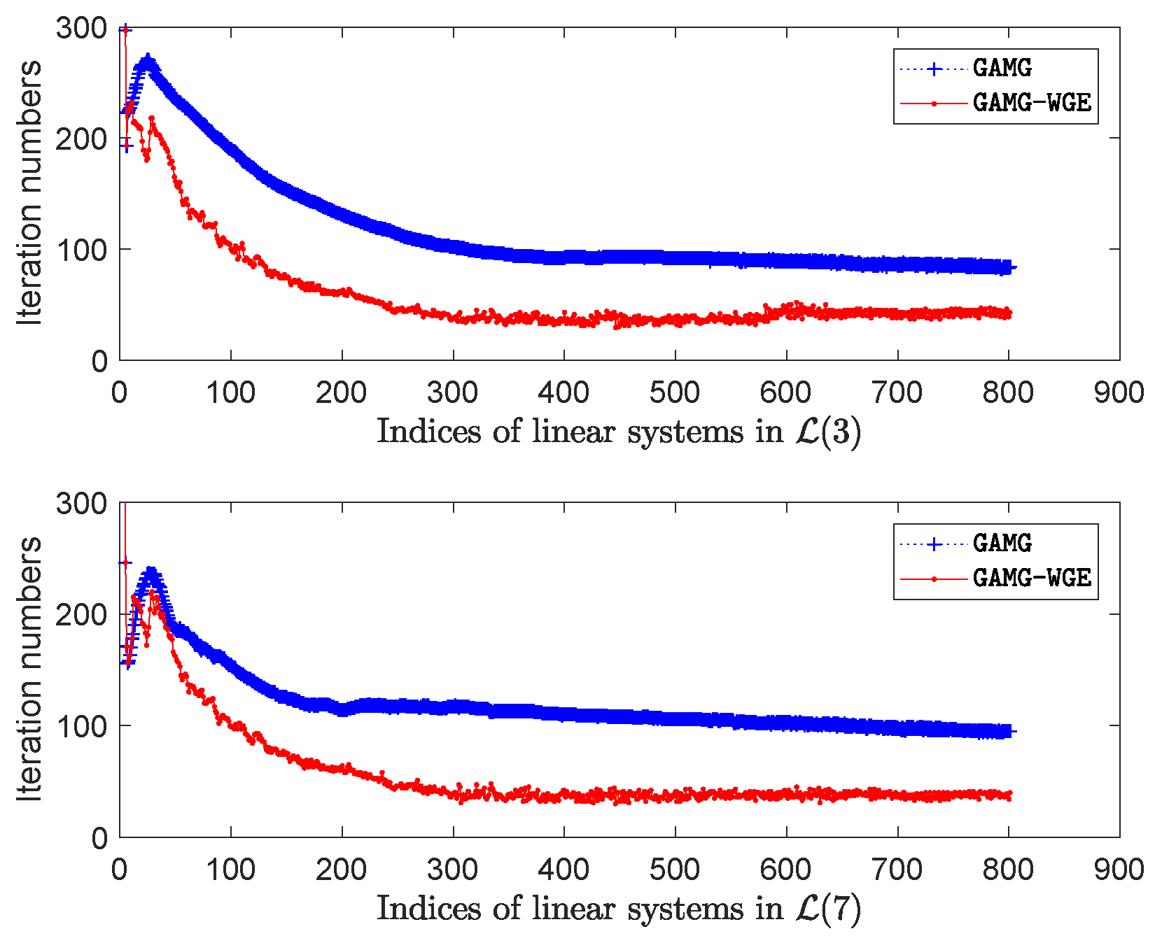Figure 17 compares the iteration number of each linear equation system in $\mathcal{L}\left(3\right)$ and $\mathcal{L}\left(7\right)$ solved by different methods. One can see that the GAMG-WGE method outperforms the GAMG method in terms of iteration number in most linear equation systems in both lanes. We report the result of the total iteration number and solution time in

Table 4. The test result of 3D blended-wing-body airfoil ${}^{†}$.

Method	$\mathit{Nits}$	${\mathit{T}}_{\mathit{total}}^{\mathit{p}}$	${\mathit{T}}_{\mathit{total}}$	${\mathit{S}}_{\mathit{p}}$	${\mathit{S}}_{\mathit{total}}$
GAMG	199,993	5749.4	6153.0	-	-
GAMG-WGE	104,894	2891.9	3283.0	1.99	1.87

${}^{†}$$Ncell=4,255,146,Nprocs=240$.

. One can see that the total iteration number of all the linear equation systems is reduced by $47.5\%$ using the GAMG-WGE method. Consequently, the total solution time of the pressure equations is reduced by $49.7\%$, and the total simulation time is reduced by $46.6\%$.

5. Conclusions

The segregated iterative method, such as PISO or PIMPLE, is widely used for the numerical solution of the incompressible Navier–Stokes equations. The solution of the pressure equation generated in PISO or PIMPLE has dominated the computational cost in the whole simulation. The most time-consuming part is to solve a series of linear equation systems arising from the pressure equation. The initial guess for the iterative solution of these linear systems has a critical impact on the solution efficient. In this paper, we target at improving the initial guess for the linear systems in incompressible flow to enhance the solution efficiency.

Generally, the previous solution is used as the initial guess for solving the following linear system. However, in PISO or PIMPLE, we observe that the solution on every single grid is oscillatory. By using this characteristic, a weighted group extrapolation method is applied to calculate a solution-closer initial guess instead of the general but poor one, the solution of the previous linear equation system. In this method, the linear equation systems in different correction steps are partitioned into lanes according to the specific setting of the solution algorithm. In addition, solutions of several previous time steps in a fixed size window in each lane are organized in groups. The solution on each cell in each lane is expected to be smooth, along with the time steps. Within a specific correction step, the corresponding groups provide predicted solutions by a linear extrapolation method. We calculate the solution-closer initial guess by taking the average of the sum of the weighted predicted solution in each group.

We implement this method based on OpenFOAM and investigate the performance and effectiveness in the incompressible flow simulation, including a 2D tutorial case called pitzDaily from OpenFOAM, a 2D NACA0012 airfoil case and a 3D blended-wing-body airfoil case. The result shows that the weighted group extrapolation method manages to obtain a better and solution-closer initial guess from groups so that the acceleration is realized compared with the original one. A maximum simulation time cost reduction reaches 61.3% in the 2D NACA0012 airfoil case. It is shown that the proposed method is useful for solving the pressure equations generated in the segregated iterative schemes while solving incompressible Navier–Stokes equations.