Article

Bayesian Derivative Order Estimation for a Fractional Logistic Model

by
Francisco J. Ariza-Hernandez
1,
Martin P. Arciga-Alejandre
1,*,
Jorge Sanchez-Ortiz
1 and
Alberto Fleitas-Imbert
2
1
Facultad de Matemáticas, Universidad Autónoma de Guerrero, Av. Lázaro Cárdenas S/N Cd. Universitaria. Chilpancingo, Guerrero C.P. 39087, Mexico
2
Departamento de Matemáticas, Universidad Carlos III de Madrid, Getafe, 28903 Madrid, Spain
*
Author to whom correspondence should be addressed.
Mathematics 2020, 8(1), 109; https://doi.org/10.3390/math8010109
Submission received: 5 December 2019 / Revised: 5 January 2020 / Accepted: 7 January 2020 / Published: 10 January 2020
(This article belongs to the Special Issue Direct and Inverse Problems for Fractional Differential Equations)

Abstract

:
In this paper, we consider the inverse problem of derivative order estimation in a fractional logistic model. In order to solve the direct problem, we use the Grünwald-Letnikov fractional derivative, then the inverse problem is tackled within a Bayesian perspective. To construct the likelihood function, we propose an explicit numerical scheme based on the truncated series of the derivative definition. By MCMC samples of the marginal posterior distributions, we estimate the order of the derivative and the growth rate parameter in the dynamic model, as well as the noise in the observations. To evaluate the methodology, a simulation was performed using synthetic data, where the bias and mean square error are calculated, the results give evidence of the effectiveness for the method and the suitable performance of the proposed model. Moreover, an example with real data is presented as evidence of the relevance of using a fractional model.

1. Introduction

Nowadays, fractional differential equations have acquired a great interest, both for their theoretical development and for their applications to different problems of Physics, Engineering, Chemistry, Biology and Applied Sciences [1,2,3]. Under certain conditions, these models can more closely describe phenomena whose dynamics in time is anomalous [4]. For example, the population growth model is one of the most popular models to describe the population growth in the time; however, when the growth is faster or slower than exponential, then its fractional version of this model has a better fit (see Ariza et al. [5]).
The problem of parameters identification in fractional model is not a easy task. There are few works related to the estimation of the order of the derivative in dynamic systems.To mention a few, Mitkowski and Obraczka [6] performed deterministic estimation of parameters in a population model of fractional order, and afterwards Obraczka and Mitkowski [7] performed parameter identification in a partial differential equation of fractional order. More recently, Ariza et al. [5] made an estimate of the parameters, from the Bayesian viewpoint, of a fractional population growth model. However, there is no evidence of the estimation of the order of the derivative of a fractional logistic model.
In this paper, our interest is to estimate the order of the derivative in a differential equation based on measurements data, under uncertainty, of the solutions of a fractional-order logistic model. For this purpose, we solve the inverse problem from point of view of the Bayesian Inference. The Bayesian approach towards inverse problems is different from the traditional methods, such as regularization methods that produce singles estimates of the parameters of interest, in the ill-posedness problem. In the statistical inversion theory via Bayesian approach, the solution of the inverse problem is the posterior probability distribution of the unknowns, which can be used to obtain estimates (see [8]).
In addition to the estimation, we do not have an analytical form of the direct problem, so a numerical algorithm is required to find numerical solutions of the model under study. For simplicity, we propose to use a numerical scheme based in the Grünwald-Letnikov definition for a the fractional derivative; however, other numerical schemes can be used, such as Heydari et al. [9]. Christen et al. [10] study the case when it is necessary to involve numerical methods to approximate the forward maps of the ordinary and partial differential equations with intractable solutions, which lead to the use of a numerical posterior distributions.
Bayesian statistical aspects in inverse problems, we can find in [8,11,12], which supply a vast bibliography on the subject. Capistran et al. [13] also performed a Bayesian analysis of inverse problems in ordinary differential equations (ODE’s). Bahaumik [14] use Bayesian two-step approach to solve inverse problem in ODE’s, that don’t have closed form analytic solution. Calvetti et al. [15] mentioned several articles on the development of Bayesian inverse problems in a wide range of applications, such as engineering, geophysics, life sciences and economy.

2. The Model

This paper deals with a model composed as follows:
  • A fractional differential equation given by
    ( 1 ) D α x ( t ) = a x ( t ) ( 1 x ( t ) N ) , a > 0 , α ( 0 , 1 ] ; x ( t 0 ) = x 0 ,
    where x ( t ) is the state variable of the system at the time t, x 0 is the initial condition, a is a positive constant and N represents a sort of “ideal” population or “carrying capacity”. Here D α is the integral operator defined by
    D α x ( t ) = 1 Γ ( 1 α ) 0 t x ( τ ) ( t τ ) α d τ ,
    where D α is known as the Caputo fractional derivative for α ( 0 , 1 ) , and Γ is the Gamma function,
  • A statistical model given by
    y i = g ( x ( t i ) ) + ε i , i = 1 , , n ,
    where ε i is a Gaussian error, y i correspond to the i-th observed value under uncertainty from a solution of Equation (1) at the discrete time t i [ 0 , T ] , i = 1 , 2 , , n ; g is the observation function.
Note that if α = 1 in the Equation (1), then we get the well known classical logistic model, with solution
x ( t ) = N x 0 x 0 + ( N x 0 ) e a t .
On the other hand, when 0 < α < 1 , we do not have an analytical solution; then, a numerical approach is required to find a numerical approximation of the direct problem. In this work, using the fact that D α x ( t ) G L D α x ( t ) (see [16]), where G L D α x ( t ) is the Grünwald-Letnikov’s derivative, defined by
G L D α x ( t ) = lim h 0 h α k = 0 ( 1 ) k ( α k ) x ( t k h ) ,
where
( α k ) = Γ ( α + 1 ) Γ ( k + 1 ) Γ ( α k + 1 ) ,
we get the following approximation, for h sufficiently small,
G L D α x ( t m ) Δ h α ( t m ) = h α k = 0 m ( 1 ) k ( α k ) x ( t m k h ) , t m = m h , m = 0 , 1 , 2 ,
Therefore, from Equations (5) and (1) we arrive to the following explicit numerical scheme,
x m h = k = 1 m ( 1 ) k + 1 ( α k ) x m k h + h α a x m 1 h ( 1 x m 1 h N ) .
In this sense, we now have a discrete model analogous to model Equation (2),
y i h = g ( x m h ( t i ) ) + ε i , i = 1 , , n .

3. Bayesian Estimation

Nowadays, the uncertainty quantification from a Bayesian perspective for the differential equations is a very interesting subject because of the great number of applications. In this paper, we study the derivative order estimation, trough Bayesian approach, for a fractional logistic model. Fan et al. [17,18] give evidence of the effectiveness to solve inverse problems under the Bayesian perspective in fractional models. In [8] we can find in detail the Bayesian approach for inverse problems. Hence, the solution to inverse problem under the Bayesian approach is find the posterior distribution of the parameter of interest, which is obtained by the Bayes’ theorem as
p ( θ | y ) = L ( y | θ ) p ( θ ) Θ L ( y | θ ) p ( θ ) d θ ,
where θ is the vector of the parameters of interest α , a and σ 2 ; y are the observations data, p ( θ ) is the prior distribution of θ , which is obtained under the assumption that α , a and σ 2 are independent random variables, so
p ( θ ) = p ( a ) p ( α ) p ( σ 2 ) ,
according to parameter space of α , a and σ 2 , we propose the prior distributions as
a Γ ( r a , λ a ) , α U ( 0 , 1 ) , τ Γ ( r τ , λ τ ) ,
where Γ ( r , λ ) is the Gamma distribution with shape parameter r and rate parameter λ and U ( 0 , 1 ) is the Uniform distribution on interval ( 0 , 1 ) , τ = 1 / σ 2 is the precision parameter and Θ = R + × ( 0 , 1 ) × R + .
The likelihood function is obtained by
L ( y | θ ) = τ n / 2 ( 2 π ) n / 2 exp { τ 2 i = 1 n ( y i g ( x ( t i ) ) ) 2 } .
where x ( t i ) , i = 1 , n is a solution from Equation (1).
In our case, when α ( 0 , 1 ) , we don’t have an explicit expression of the solution in Equation (1). Thus, instead of x ( t ) , we use a numerical approximation x h given by Equation (6) in Equation (9), in order to obtain a new likelihood function L h ( y | θ ) . Then, from now ahead our statistical inference is going to come from a new posterior distribution p h ( θ | y ) L h ( y | θ ) p ( θ ) [13].
In order to approximate p h ( θ | y ) we implement Markov Chain Monte Carlo (MCMC) methods, using JAGS within the R software [19]. For more details about the JAGS package see [20,21,22]. For Bayesian point estimation, we use the MAP estimator of θ , i.e.,
θ ^ B = arg max θ Θ p h ( θ | y ) .
To draw samples from the posterior distribution, JAGS use the Gibbs sampling and sometimes it is combined or replaced by complex techniques such that Metropolis-Hastings algorithm, Slice sampling [23] and Adaptive Rejection Sampling.

4. Simulation

In this section, we carried out a simulation study to give evidence of the properties of Bayesian estimators in the context of the inverse problem for fractional logistic model ( M 1 ) in the presence of the ordinary logistic model ( M 2 ) misspecification. For this task, we used R [19] with R2jags package [21], following the procedure below:
  • We generated 1000 synthetic data sets from the fractional logistic model using a = 1 , σ 2 = 30 , X 0 = 20 and for the values α = 0.25 , 0.5 , 0.75 , for two sample sizes, n = 25 and n = 50 , and h = 0.16 and 0.08 , respectively. Each data set was simulated using the model defined in Equations (6) and (7) and g as identity function.
  • We calculated the MAP estimators of the parameters for the models M 1 and M 2 . To make inference, we use a total of 2000 iterations for each parameter of interest, with two chains of length 10,000 each one. We propose the following weakly informative prior distributions [24],
    a Γ ( 0.001 , 0.001 ) , α U ( 0 , 1 ) , τ Γ ( 0.001 , 0.001 ) .
  • From the 1000 samples, we obtained measures of the bias and mean-squared error of the estimators.
For each simulation, we carried out standard convergence diagnostics, such as the factor of reduction, the Gelman-Rubin factor and Geweke diagnostics, which were calculated and showed evidence of convergence. In Table 1, we report the estimate bias and estimate mean squared error for the cases considered. In the fractional logistic model, both the bias and mean squared error are very close to the zero value in all the cases studied, as expected. In contrast, if we use the ordinary logistic model for the same data, the bias and mean squared error are less accurate compared to the fractional logistic model. Moreover, we can observe that the bias and mean squared error are increasing when the α value tends to zero.
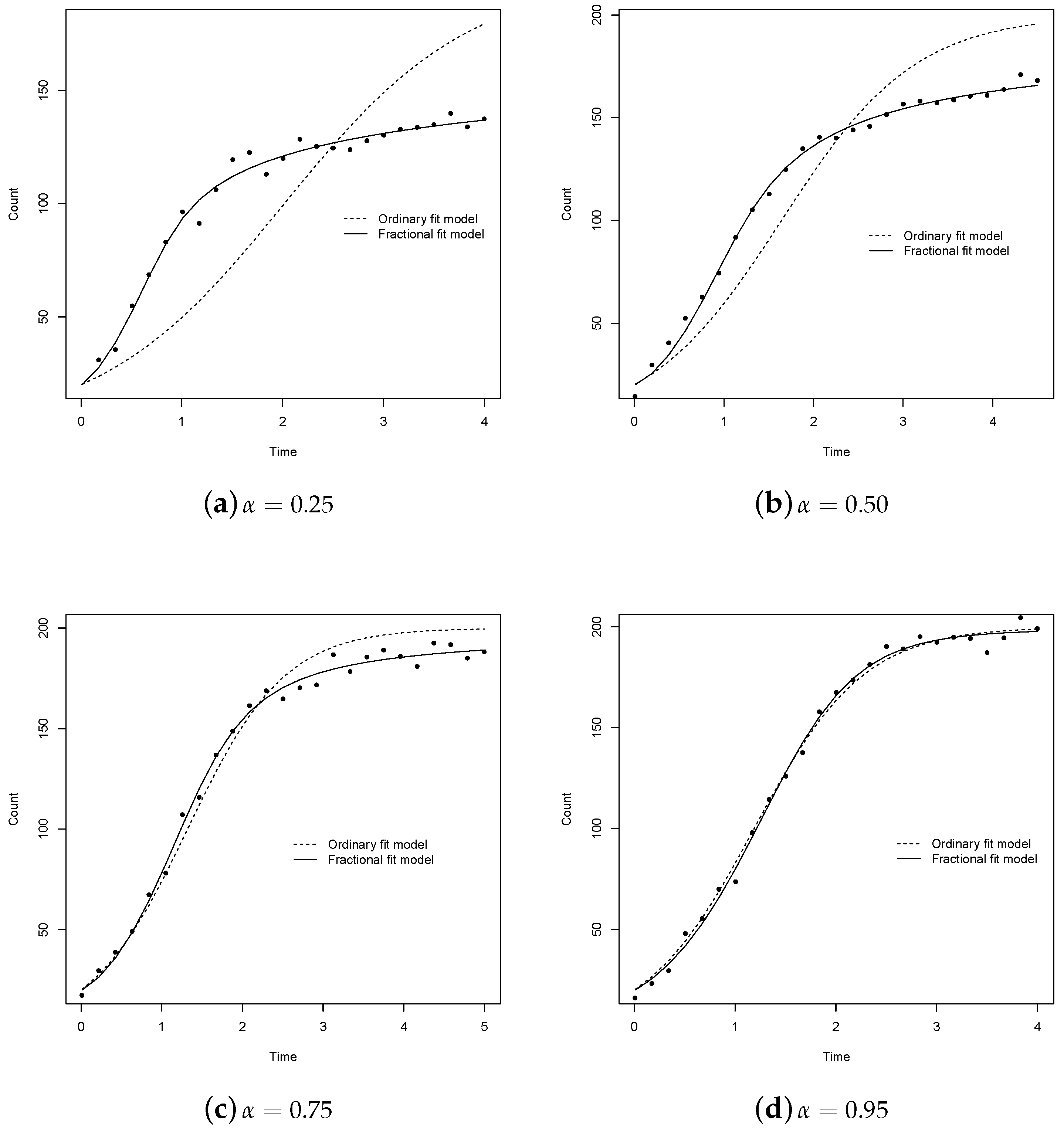
In Figure 1 we present, as an example, four sets of synthetic data from the model Equations (6) and (7) generated with values of the parameters a = 1 , σ 2 = 30 , n = 25 , h = 0.16 and α = 0.25 , 0.50 , 0.75 , 0.95 , respectively.

5. Illustrative Example

An example with real data is given to illustrate the Bayesian estimation of the derivative order in the fractional logistic model proposed in this paper. The observation data consists of 15 measurements of electric power (in kilowatts) from 20 serial connected solar panels of 255 watts each one. This data was obtained each 20 minutes from 9:20 to 14:00 hours using, a 5 kW digital inverter on July 27, 2018, in Acapulco, Mexico.
At a first glance (see Figure 2), we can observe a S-shape behaviour of the data; however, the ordinary logistic model is unable to fit the data accurately. Then, to tackle this problem we add a parameter for the order of the derivative.
For this example, we used two chains, each with 500,000 iterations, and the first 250,000 were discarded, taking a thinning rate of 50. Thus, 10,000 posterior samples were used to obtain the summary statistics about the parameters of interest. The prior distributions used were for α U ( 0 , 1 ) , a Γ ( 0.001 , 0.001 ) and 1 / σ 2 Γ ( 0.001 , 0.001 ) . We carried out standard convergence diagnostics, the values of factor reduction for each parameter were close to 1 for both models. Also, the Gelman-Rubin factor and Geweke diagnostics were calculated and showed evidence of convergence. As Bayesian point estimates of the parameters were used the posterior means, resulting, for M 1 : α ^ = 0.95 , a ^ = 0.12 and σ ^ 2 = 0.02 , for M 2 : a ^ = 0.08 and σ ^ 2 = 0.07 . Figure 2, shows the fitted models considered.
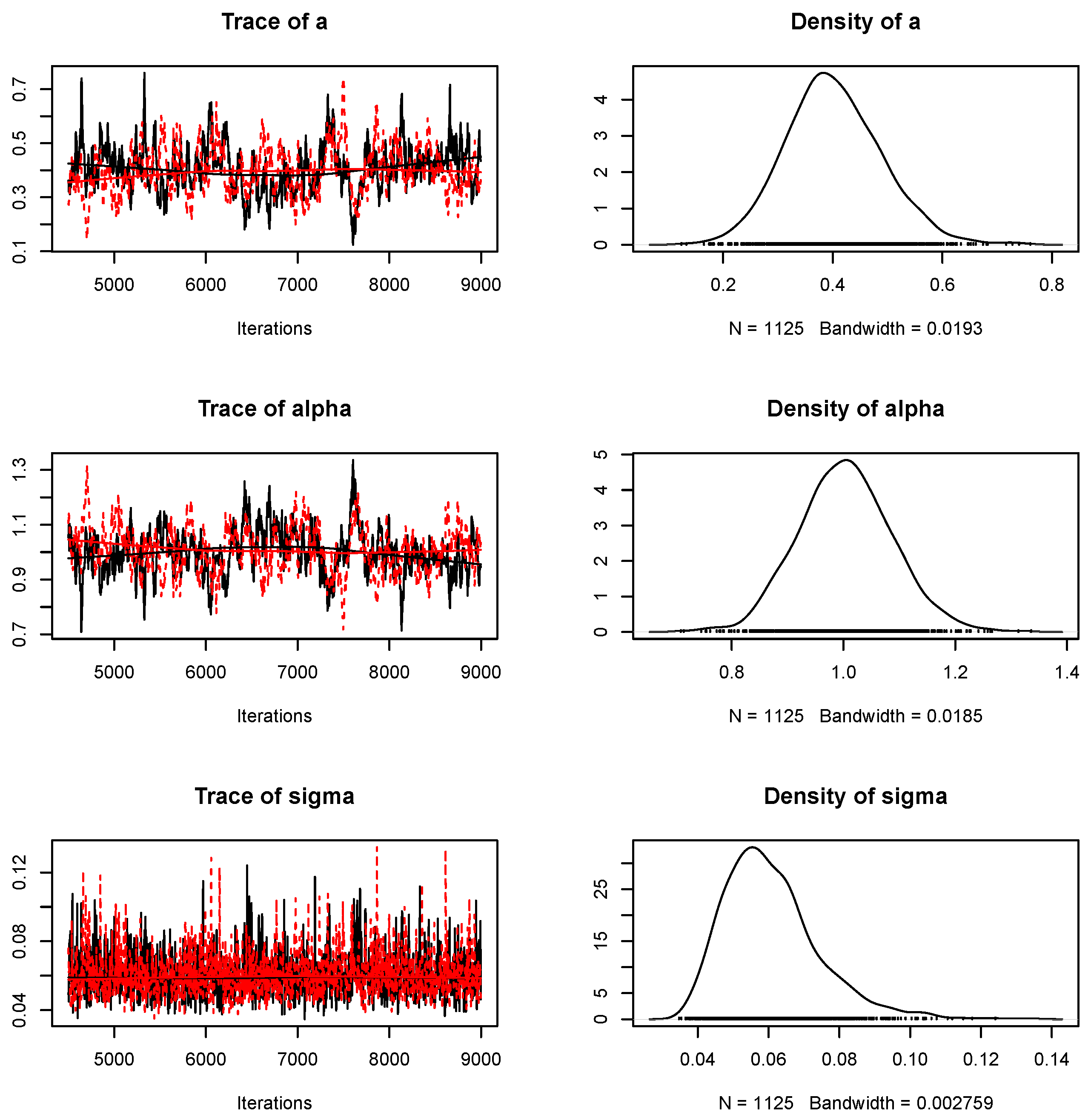
The Figure 3, shows the trace and estimated posterior distributions of the estimated parameters of interest.

6. Concluding Remarks

In this paper, taking into account an experimental dataset with noise, we solve an inverse problem for a fractional logistic model via the Bayesian perspective, where the derivative order is included as a parameter of interest; that is, the order of the derivative is considered as a random variable, with a non-informative prior probability density function in the interval (0, 1). Then, we implement MCMC methods to obtain the posterior probability distribution for the derivative order and its point estimator is given by the mean of the posterior distribution. Since, it is not possible to find an analytical solution for the corresponding initial value problem, a numerical scheme was proposed, based on the definition of Grünwald-Letnikov’s fractional derivative, to solve the direct problem in each MCMC iteration, obtaining accurate numerical posterior distributions of the parameters in the following sense: from the simulation study, the biases and mean squared errors are close to zero.
In this work, deals with the problem of parameters estimation in differential equations using Bayesian statistical inference tools, which is a new subject with many interesting open problems and potential applications in different areas of knowledge. Also, the procedure that we propose can be used for mathematical problems based on system of fractional partial differential equations.

Author Contributions

Conceptualization, F.J.A.-H. and M.P.A.-A.; Formal analysis, M.P.A.-A. and J.S.-O.; Investigation, F.J.A.-H. and J.S.-O.; Methodology, F.J.A.-H. and A.F.-I.; Software, A.F.-I.; Writing—original draft, F.J.A.-H. and A.F.-I.; Writing—review and editing, M.P.A.-A. and J.S.-O. All authors have read and agreed to the published version of the manuscript.

Funding

This research was funded by University of Guerrero, Mexico., grant number PFCE-2019.

Conflicts of Interest

The authors declare no conflict of interest.

References

  1. Monje, C.A.; Chen, Y.; Vinagre, B.M.; Xue, D.; Feliu-Batlle, V. Fractional-Order Systems and Controls: Fundamentals and Applications; Springer: Berlin/Heidelberg, Germany, 2010. [Google Scholar]
  2. Vazquez, L.; Trujillo, J.J.; Velasco, M.P. Fractional heat equation and the second law of thermodynamics. Fract. Calc. Appl. Anal. 2011, 14, 334–342. [Google Scholar] [CrossRef]
  3. Area, I.; Batarfi, H.; Losada, J.; Nieto, J.J.; Shammakh, W.; Torres, A. On a fractional order Ebola epidemic model. Adv. Differ. Equ. 2015, 2015, 278. [Google Scholar] [CrossRef] [Green Version]
  4. Jin, B.; Rundell, W. A tutorial on inverse problems for anomalous diffusion processes. Inverse Probl. 2015, 31, 035003. [Google Scholar] [CrossRef] [Green Version]
  5. Ariza-Hernandez, F.J.; Sanchez-Ortiz, J.; Arciga-Alejandre, M.P.; Vivas-Cruz, L.X. Bayesian Analysis for a Fractional Population Growth Model. J. Appl. Math. 2017, 2017, 9654506. [Google Scholar] [CrossRef]
  6. Mitkowski, W.; Obraczka, A. Simple identification of fractional differential equation. Solid State Phenom. 2012, 180, 331–338. [Google Scholar] [CrossRef]
  7. Obraczka, A.; Mitkowski, W. The comparison of parameter identification methods for fractional, partial differential equation. Solid State Phenom. 2014, 210, 265–270. [Google Scholar] [CrossRef]
  8. Kaipio, J.; Somersalo, E. Statistical and Computational Inverse Problems; Springer: Berlin/Heidelberg, Germany, 2006; Volume 160. [Google Scholar]
  9. Heydary, M.H.; Hooshmandasl, M.R.; Cattani, C.; Li, M. Legendre Wavelets Method for Solving Fractional Population Growth Model in a Closed System. Math. Probl. Eng. 2013, 2013, 161030. [Google Scholar] [CrossRef] [Green Version]
  10. Andrés Christen, J.; Capistrán, M.A.; Ángel Moreles, M. Numerical posterior distribution error control and expected Bayes Factors in the bayesian Uncertainty Quantification of Inverse Problems. arXiv 2016, arXiv:1607.02194. [Google Scholar]
  11. Banks, H.T.; Hu, S.; Thompson, W.C. Modeling and Inverse Problems in the Presence of Uncertainty; CRC Press: Boca Raton, FL, USA, 2014. [Google Scholar]
  12. Tarantola, A. Inverse Problem Theory and Methods for Model Parameter Estimation; SIAM: Philadelphia, PA, USA, 2005. [Google Scholar]
  13. Capistrán, M.A.; Christen, J.A.; Donnet, S. Bayesian Analysis of ODE’s: Solver Optimal Accuracy and Bayes factors. SIAM/ASA J. Uncertain. Quantif. 2016, 4, 829–849. [Google Scholar] [CrossRef] [Green Version]
  14. Bhaumik, P. Bayesian two-step estimation in differential equation models. Electron. J. Stat. 2015, 9, 3124–3154. [Google Scholar] [CrossRef]
  15. Calvetti, D.; Kaipio, J.P.; Somersalo, E. Inverse problems in Bayesian framework. Inverse Probl. 2014, 30, 110301. [Google Scholar] [CrossRef] [Green Version]
  16. Scherer, R.; Kalla, S.L.; Tang, Y.; Huang, J. The Grunwald- Letnikov method for fractional differential equations. Comput. Math. Appl. 2011, 62, 902–917. [Google Scholar] [CrossRef] [Green Version]
  17. Fan, W.; Jiang, X.; Chen, S. Parameter estimation for the fractional fractal diffusion model based on its numerical solution. Comput. Math. Appl. 2016, 71, 641–651. [Google Scholar] [CrossRef]
  18. Fan, W.; Jiang, X.; Qi, H. Parameter estimation for the generalized fractional element network Zener model based on the Bayesian method. Physica A 2015, 427, 40–49. [Google Scholar] [CrossRef]
  19. R Core Team. R: A Language and Environment for Statistical Computing; R Foundation for Statistical Computing: Vienna, Austria, 2014. [Google Scholar]
  20. Plummer, M. JAGS Version 4.3.0 User Manual; International Agency for Research on Cancer: Lyon, France, 2017. [Google Scholar]
  21. Su, Y.S.; Yajima, M. R2jags: Using R to Run ‘JAGS’. R Package Version 0.5-7. Available online: https://CRAN.R-project.org/package=R2jags (accessed on 1 December 2019).
  22. Plummer, M. rjags: Bayesian Graphical Models Using MCMC. R Package Version 4-6. Available online: https://CRAN.R-project.org/package=rjags (accessed on 1 December 2019).
  23. Neal, R.M. Slice Sampling. Ann. Stat. 2003, 31, 705–767. [Google Scholar] [CrossRef]
  24. Gelman, A.; Carlin, J.B.; Stern, H.S.; Dunson, D.B.; Vethari, A.; Rubin, D.B. Bayesian Data Analysis, 3rd ed.; Taylor & Francis: Milton Park, UK, 2014. [Google Scholar]
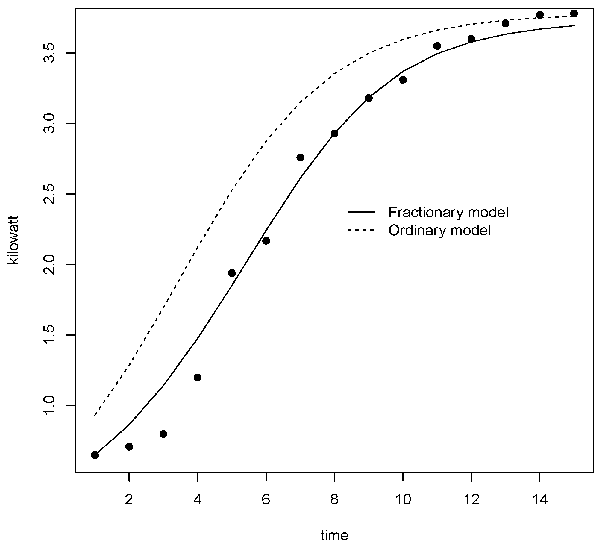
Figure 1. Synthetic data from the model Equations (6) and (7).
Mathematics 08 00109 g001
Figure 2. Data panel.
Mathematics 08 00109 g002
Figure 3. Trace and estimated posterior densities of a, α and σ .
Mathematics 08 00109 g003
Table 1. Estimation of Bias and MSE.
Sample SizeParameter M 1 M 2
BiasMSEBiasMSE
n = 25 α = 0.25
a−0.000480.000040.4460.199
α −0.000880.00005
σ 2 −0.014100.00021−0.2880.081
α = 0.5
a0.000420.000060.2830.082
α −0.000370.00001
σ 2 −0.013500.00019−0.1900.037
α = 0.75
a0.000830.000070.1450.022
α −0.000970.00014
σ 2 −0.013300.00019−0.0860.008
n = 50 α = 0.25
a−0.000140.000020.4330.188
α −0.000040.00003
σ 2 −0.007100.00006−0.3100.095
α = 0.5
a0.000490.000020.2940.087
α −0.000220.00005
σ 2 −0.006400.00005−0.1780.032
α = 0.75
a0.000740.0000350.1780.032
α −0.000520.00830
σ 2 −0.006500.00005−0.0690.005