Abstract
In high-dimensional data, the performances of various classifiers are largely dependent on the selection of important features. Most of the individual classifiers with the existing feature selection (FS) methods do not perform well for highly correlated data. Obtaining important features using the FS method and selecting the best performing classifier is a challenging task in high throughput data. In this article, we propose a combination of resampling-based least absolute shrinkage and selection operator (LASSO) feature selection (RLFS) and ensembles of regularized regression (ERRM) capable of dealing data with the high correlation structures. The ERRM boosts the prediction accuracy with the top-ranked features obtained from RLFS. The RLFS utilizes the lasso penalty with sure independence screening (SIS) condition to select the top k ranked features. The ERRM includes five individual penalty based classifiers: LASSO, adaptive LASSO (ALASSO), elastic net (ENET), smoothly clipped absolute deviations (SCAD), and minimax concave penalty (MCP). It was built on the idea of bagging and rank aggregation. Upon performing simulation studies and applying to smokers’ cancer gene expression data, we demonstrated that the proposed combination of ERRM with RLFS achieved superior performance of accuracy and geometric mean.
Keywords:
ensembles; feature selection; high-throughput; gene expression data; resampling; lasso; adaptive lasso; elastic net; SCAD; MCP MSC:
62P10; 62F40; 62F07
1. Introduction
With the advances of high throughput technology in biomedical research, large volumes of high-dimensional data are being generated [1,2,3]. Some of the examples of what produces such data are microarray gene expression [4,5,6] data sequencing, RNA-seq [7], genome-wide association studies (GWASs) [8,9], and DNA-methylation studies [10,11]. These data are high dimensional in nature, where the total count of features is significantly larger than the number of samples —termed the curse of dimensionality. Although this is one of the major problems, there are many other problems, such as noise, redundancy, and over parameterization. To deal with these problems, many two-stage approaches of feature selection (FS) and classification algorithms have been proposed in machine learning over the last decade.
The FS methods are used to reduce the dimensionality of data by removing noisy and redundant features that help in selecting the truly important features. The FS methods are classified into rank-based and subset methods [12,13]. Rank-based methods rank all the features with respect to their importance based on some criteria. Although there is a lack of threshold to select the optimal number of top-ranked features, this can be solved using the sure independence screening (SIS) [14] conditions. Some of the popular rank-based FS methods used in bioinformatics are information gain [15], Fisher score [16], chi-square [17], and minimum redundancy maximum relevance [18]. These rank-based FS methods have several advantages, such as that they avoid overfitting and are computationally faster because they do not depend on the performances of classification algorithms. However, these methods do not consider joint importance because they focus on marginal significance. To overcome this issue, feature subset section methods were introduced. The subset methods [19] are the ones where the subsets of features are selected with some predetermined threshold based on some criteria, but these methods need more computational time in a high-dimensional data setting and lead to an NP-hard problem [20]. Some of the popular subset methods include Boruta [21] and relief [22].
For the classification of gene expression data, there are non-parametric-based popular algorithms, such as random forests [23], Adaboost [24], and support vector machines [25]. The support vector machines are known to perform well in highly correlated gene expression data compared to the random forests [26]. The random forests and Adaboost are based on the concept of decision trees, and the support vector machines are based on the idea of hyperplanes. In addition to the above, there are parametric machine learning algorithms, such as penalized logistic regression (PLR) models, that have five different penalties which are predominantly popular in high-dimensional data. The first two classifiers are Lasso [27] and ridge [28] that are based on L1 and L2 penalties. The third classifier is a combination of these and is termed as elastic net [29]. The other two PLR classifiers are SCAD [30] and MCP [31], which are based on non-concave and concave respectively. All these individual classifiers are very common in machine learning and bioinformatics [32]. However, in highly correlated gene expression data, the individual classifiers do not perform well in terms of prediction accuracy. To overcome the issue of individual classifiers, ensemble classifiers are proposed [33,34]. The ensemble classifiers are bagging and aggregating methods [35,36] that are employed to improve the accuracy of several “weak” classifiers [37]. The tree-based method of classification by ensembles from random partitions (CERP) [38] showed good performance but is computer-intensive. The ensembles of logistic regression models (LORENS) [39] for high-dimensional data were proven to be better for classification. However, there was a decrease in performance when there were a smaller number of true, important variables in the high-dimensional space because of random partitioning.
To address these issues, there is a need to develop a novel combination of FS with a classification method and compare the proposed method with the other combinations of popular FS with the classifiers through extensive simulation studies and a real data application. In a high dimensional data set, it is necessary to filter out the redundant and unimportant features using the FS methods. This helps in reducing the computational time and helps in boosting the prediction accuracy with the help of significant features.
In this article, we introduce the combination of an ensemble classifier with an FS method—the resampling-based lasso feature selection (RLFS) method for ranking features, and ensemble of regularized regression models (ERRM) for classification purposes. The resampling approach was proven to be one of the best FS screening steps in a high-dimensional data setting [13]. The RLFS uses the selection probability with lasso penalty, and the threshold for selecting the top-ranked features is set using b-SIS condition; and these select features were applied to the ERRM to achieve the best prediction accuracy. The ERRM uses five individual regularization models, lasso, adaptive lasso, elastic net, SCAD, and MCP.
2. Materials and Methods
The FS method includes the proposed RLFS method, information gain, chi-square, and minimum redundancy maximum relevance. The classification methods include support vector machines, penalized regression models, and tree-based methods, such as random forests and adaptive boosting. The programs for all the experiments were written using R software [40]. The FS and classification were performed with the packages [41,42,43,44,45,46] obtained from CRAN. The weighted rank aggregation was evaluated with the RankAggreg package obtained from [47]. The codes for implementing the algorithms are available at [48]. The SMK-CAN-187 data were obtained from [49]; some of the applications of the data can be found in the articles [50,51] where the importance of screening approach in high dimensional data is elaborated.
2.1. Data Setup
To assess the performances of the models, we developed simulation study and also considered a real application of gene expression data.
2.1.1. Simulation Data Setup
The data were generated based on a random multivariate normal distribution where the mean was assigned as 0, and the variance-covariance matrix adapts a compound symmetry structure with the diagonal items set to 1 and the off-diagonal items being values.
The class labels were generated using the Bernoulli trails with the following probability:
The data matrix was generated using the random multivariate normal distribution, and the response variable was generated by binomial distribution, as shown in Equations (1) and (2) respectively. For sufficient comparison of the performance of the model and subsidizing the effects of the data splits, all of the regularized regression models were built using the 10-fold cross-validation procedure, and the averages were taken over 100 partitioning times referred to as 100 iterations in this paper. The data generated are high-dimensional in nature with the number of samples, n = 200 and total features, p = 1000. The true regression coefficients were set to 25, which were generated using uniform distribution with the minimum and maximum values 2 and 4, respectively.
With this setup of high-dimensional data, we simulated three different types of data, each with correlation structures = 0.2, 0.5, and 0.8 respectively. These values show the low, intermediate, and high correlation structures in the datasets which are significantly similar to what we usually see in the gene expression or others among many types of data in the field of bioinformatics [13,52]. At first, the data were divided randomly into training and testing sets with 75% and 25% of samples respectively; 75% of the training data was given to the FS methods, which ranked the genes concerning their importance, and then the top-ranked genes were selected based on b-SIS condition. The selected genes were applied in all the classifiers. For standard comparison and mitigating the effects of the data splitting, all of the regularized regression models were built using the 10-fold cross-validation; the models were assessed for testing the performance with the testing data using different evaluation metrics, and averages were taken over 100 splitting times referred to as 100 iterations.
2.1.2. Experimental Data Setup
To test the performance of the proposed combination of ERRM with RLFS, and compare it with the rest of the combinations of FS and classifiers, the gene expression data SMK-CAN-187 were analyzed. The data include 187 samples and 19,993 genes obtained from smokers, which included 90 samples from those with lung cancer and 97 samples from those without lung cancer. This data is high-dimensional, with the number of genes being 19,993. The preprocessing procedures are necessary to handle these high-dimensional data. At first, the data were randomly divided into training and testing sets with 75% and 25% of samples respectively. As the first filtering step, 75% of the training data were given to the marginal maximum likelihood estimator (MMLE), to overcome the redundant noisy features, and the genes were ranked based on their level of significance. The ranked significant genes were next applied to the FS methods along with the proposed RLFS method as the second filtering step, and a final list of truly significant genes was obtained. These significant genes were applied to all the classification models along with the proposed ERRM classifier. All of the models were built using the 10-fold cross-validation. The average classification accuracy and Gmean of our proposed framework were tested using the test data. The above procedure was repeated for 100 times and the averages were taken.
2.1.3. Data Notations
Let the expression levels of features in ith sample be represented as for , where n is the total number of samples and p is the total number of features. The response variables, , where = 0 means that ith individual is in the non disease group and = 1 is disease group.
The original data were split into for the training set and for the testing set . The training set for , where t is the number of training samples, the response variable for the training set. The testing set for , where v is the number of testing samples; the response variable is for the testing set. The classifiers are fitted on , and the class labels as training data set to predict the classification of using of the testing set.
The detailed procedure is as follows. The training data were given to the FS methods, and the new reduced feature set for , where t was the samples included in training data, and f was the reduced number of features after the FS step. This reduced feature set was used as new training data for building the classification models.
2.2. Rank Based Feature Selection Methods
With the gain in popularity of high dimensional data in bioinformatics, the challenges to deal with it also grew. In gene expression data, having large p and small n problems, the n represents the samples as patients and p represents the features as genes. Dealing with such a large number of genes that are generated by conducting large biological experiments involves computationally intensive tasks that become too expensive to handle. The performance drops when such a large number of genes are added to the model. To overcome this problem, employing FS methods becomes a necessity. In statistical machine learning, there are many FS methods developed to deal with the gene expression data. But most of the existing algorithms are not completely robust applications to the gene expression data. Hence, we propose an FS method that ranks the features based on some criteria explained in the next section. We also explain some other popular FS methods in classification problems, such as information gain, chi-square, and minimum redundancy maximum relevance.
2.2.1. Information Gain
The information gain (IG) method [15] is simple, and one of the widely used FS methods. This univariate FS method is used to assess the quantity of information shared between the training feature set for , where t is the number of training samples, for , where g is the feature in p number of features, and the response variable . It provides an ordered ranking of all the features having a strong correlation with the response variable that helps to obtain good classification performance.
The information gain between the gth feature in and the response variable is given as follows:
where is entropy of and is entropy of given . The entropy [53] of is defined by the following equation:
where g indicates discrete random variable and gives the probability of g on all values of . Given the random variable , the conditional entropy of is:
where is the prior probability of ; is conditional probability of g in a given y that shows the uncertainty of given .
where is the joint probability of g and y. IG is symmetric such that , and is zero if the variables and are independent.
2.2.2. Chi-Square Test
The chi-square test (Chi2) belongs to the category of the non-parametric test, which is used mainly in determining the significant relation between two categorical variables. As part of the preprocessing step, we used the “equal interval width” approach to transform the numerical variables into categorical counterparts. The “equal interval width” algorithm first divides the data into q intervals of equal size. The width of each interval is defined as: and the interval boundaries are determined by: .
The general rule in Chi2 is that the features have a strong dependency on the class labels selected, and the features independent of the class labels are ignored.
From the training set, , , where g is every feature in p number of features. Given a particular feature g with r different feature values [53], the Chi2 score of that particular feature can be calculated as:
where is the number of instances with the feature value given feature g. In addition, , where indicates the number of data instances with the feature value given feature g, denotes the number of data instances in r, and p is total number of features.
When two features are independent, the is closer to the expected count ; consequently, we will have smaller Chi2 score. On the other hand, the higher Chi2 score implies that the feature is more dependent on the response and it can be selected for building the model during training.
2.2.3. Minimum Redundancy Maximum Relevance
The minimum redundancy and maximum relevance method (MRMR) is built on optimization criteria of mutual information (redundancy and relevance); hence, it is also defined under mutual information based methods. If a feature has uniformly of expressions or if they are randomly distributed in different classes, its mutual information with such classes is null [18]. If a feature is expressed differentially for different classes, it should have strong mutual information. Hence, we use mutual information as a measure of the relevance of features. MRMR also reduces the redundant features from the feature set. For a given set of features, it tries to measure both the redundancy among features and relevance between features and class vectors.
The redundancy and relevance are calculated based on mutual information, which is as follows: We know that, in the training set , represents every feature in and is the response variable.
In the following equation, for simplicity, let us consider the training set as X and response variable as Y. The objective function is shown below:
where S is the subset of selected features and is the ith feature. The first term is a measure of relevance that is the sum of mutual information of all the selected features in the set S with respect to the output Y. The second term is measure of redundancy that is the sum of the mutual information between all the selected features in the subset S. By optimizing the Equation (9), we are maximizing the first term and minimizing the second term simultaneously.
2.3. Classification Algorithms
Along with gene selection, improving prediction accuracy when dealing with high-dimensional data has always been a challenging task. There is a wide range of popular classification algorithms used when dealing with high throughput data, such as tree-based methods [54], support vector machines, and penalized regression models [55]. These popular models are discussed briefly in this section.
2.3.1. Logistic Regression
Logistic regression (LR) is perhaps one of the primary and popular models used while dealing with binary classification problems [56]. Logistic regression for dealing with more than two classes is called multinomial logistic regression. The primary focus here is on the binary classification. Given the set of inputs, the output is a predicted probability that the given input point belongs to a particular class. The output is always within [0, 1]. Logistic regression is based on the assumption that the original input space can be divided into two separate regions, one for each class, by a plane. This plane helps to discriminate between the dots belonging to different classes and is called as linear discriminant or linear boundary.
One of the limitations is the number of parameters that can be estimated needs to be smaller and should not exceed the number of samples.
2.3.2. Regularized Regression Models
Regularization is a technique used in logistic regression by employing penalties to overcome the limitations of dealing with high-dimensional data. Here, we discuss the PLR models such as lasso, adaptive lasso, elastic net, SCAD, and MCP. These five methods are included in the proposed ERRM and also tested as independent classifiers for comparing performance with the ERRM.
The logistic regression equation:
where and .
From logistic regression Equation (10), the log-likelihood estimator is shown as below:
Logistic regression offers the benefit by simultaneous estimation of the probabilities and for each class. The criterion for prediction is , where is an indicator function.
The parameters for PLR are estimated by minimizing above function:
where is a penalty function, is the log-likelihood function.
Lasso is a widely used method in variable selection and classification purposes in high dimensional data. It is one of the five methods used in the proposed ERRM for classification purposes. The LASSO penalized regression method is defined below:
where f is the reduced number of features; is the tuning parameter that controls the strength of the L1 penalty.
The oracle property [30] has consistency in variable selection and asymptotic normality. The lasso works well in subset selection; however, it lacks the oracle property. To overcome this, different weights are assigned to different coefficients: this describes a weighted lasso called adaptive lasso. The adaptive lasso (ALASSO) penalty is shown below:
where f is the reduced number of features, is the tuning parameter that controls the strength of the L2 penalty, and is the weight vector based on ridge estimator. The ridge estimator [28] uses the L2 regularization method which obtains the size of coefficients by adding the L2 penalty.
The elastic net (ENET) [57] is the combination of lasso which uses the L1 penalty, and ridge which uses the L2 penalty. The sizable number of variables is obtained, which helps in avoiding the model turning into an excessively sparse model.
The ENET penalty is defined as:
where is the tuning parameter that controls the penalty, f is the number of features, is the mixing parameter between ridge and lasso .
The smoothly clipped absolute deviation penalty (SCAD) [30] is a sparse logistic regression model with a non-concave penalty function. It improves the properties of the L1 penalty. The regression coefficients are estimated by minimizing the log-likelihood function:
In Equation (16) the is defined by:
Minimax concave penalty (MCP) [31] is very similar to the SCAD. However, the MCP relaxes the penalization rate immediately, while for SCAD, the rate remains smooth before it starts decreasing. The MCP equation is given as follows:
In Equation (18) the is defined as:
2.3.3. Random Forests
The random forest (RF) [23] is an interpretive and straightforward method commonly used for classification purposes in bioinformatics. It is also known for its variable importance ranking in high dimensional data sets. RF is built on the concept of decision trees. Decision trees are usually more decipherable when dealing with binary responses. The idea of RF is to operate as an ensemble instead of relying on a single model. RF is a combination of a large number of decision trees where each tree has some random subset of features obtained from the data by allowing repetitions. This process is called bagging. The majority voting scheme is applied by aggregating all the tree models and obtaining one final prediction.
2.3.4. Support Vector Machines
Support vector machines (SVM) [25] are well known amongst most of the mainstream algorithms in supervised learning. The main goal of a SVM is to choose a hyperplane that can best divide the data in the high dimensional space. This helps to avoid overfitting. The SVM detects the maximum margin hyperplane, the hyperplane that maximizes the distance between the hyperplane, and the closest dots [58]. The maximum margin indicates that the classes are well separable and correctly classified. It is represented as a linear combination of training points. As a result, the decision boundary function for classifying points as to hyperplane only involves dot products between those points.
2.3.5. Adaboost
Adaboost is also known as adaptive boosting (AB) [24]. It improves the performance of a particular weak boosting classifier through an iterative process. This ensemble learning algorithm can be extensively applied to classification problems. The primary objective here is to assign more weights to the patterns that are harder to classify. Initially, the same weights are assigned to each training item. The weights of the wrongly classified items are incremented while the weights of the correctly classified items are decreased in each iteration. Hence, with the additional iterations and more classifiers, the weak learner is bound to cast on the challenging samples of the training set.
2.4. The Proposed Framework
We propose a combination of the FS method and classification method. For the filtering procedure, the resampling-based lasso feature selection method is introduced, and for the classification, the ensemble of regularized regression models is developed.
2.4.1. The Resampling-Based Lasso Feature Selection
From [13], we see that the resampling-based FS is relatively more efficient in comparison to the other existing FS methods in gene expression data. The RLFS method is based on the lasso penalized regression method and the resampling approach employed to obtain the ranked important features using the frequency.
The least absolute shrinkage and selection operator (LASSO) [27] estimator is based on L1-regularization. The L1-regularization method limits the size of coefficients pushes the unimportant regression coefficients to zero by using the L1 penalty. Due to this property, variable selection is achieved. It plays a crucial role in achieving better prediction accuracy along with the gene selection in bioinformatics.
The selection probability of the features based on the lasso is shown in the below equation.
The b-SIS criteria to select the top k ranked features is defined by,
where R is defined by the total number of resampling, L is total number of values, is the feature indexed as i, p is total number of features, n is total number of samples, and is defined as regression coefficient of mth feature and indicator variable. Each R number of resamples and L number of values of are considered to build the variable selection model. The 10-fold cross validation is considered while building the model.
After ranking the features using the RLFS method, we employ the b-SIS approach to select the top features based on Equation (22) where b is set to two. The number of true important variables selected among the top b-SIS ranked features is calculated in each iteration and the average of this is taken over 100 iterations.
2.4.2. The Ensembles of Regularized Regression Models
LASSO, ALASSO, ENET, SCAD, and MCP are the five individual regularized regression models included as base learners in our ERRM. The role of bootstrapped aggregation or bagging is to reduce the variance by averaging over an “ensemble” of trees, which will improve the performance of weak classifiers. is the number of random bootstrapped samples obtained from reduced training set with corresponding class label . The five regularized regression models are trained on each bootstrapped sample B named sub-training data, leading to models. These five regularized models are then trained using the 10-fold cross-validation to predict the classes on the out of bag samples called sub-testing data where the best model fit in each of the five regularized regression model is obtained. Henceforth, in each of the five regularized models, the best model is selected and the testing data is applied to obtain the final list of predicted classes for each of these models. For binary classification problems, in addition to accuracy, the sensitivity and specificity are primarily sought. The E evaluation metrics are computed for each of these best models of five regularized models. In order to get an optimized classifier using all the evaluation measures E is essential, and this is achieved using weighted rank aggregation. Here, each of the regularized models is ranked based on the performance of E evaluation metrics. The models are ranked based on the increasing order of performance; in the case of a matching score of accuracy for two or more models, other metrics such as sensitivity and specificity are considered. The best performing model among the five models is obtained based on these ranks. This procedure is repeated to obtain the best performing model in each of the tree T. Finally, the majority voting procedure is applied over the T trees to obtain a final list of predicted classes. The test class label is applied to measure the final E measures for assessing the performance of the proposed ensembles. The Algorithm 1 defines the proposed ERRM procedure.
The complete workflow of the proposed RLFS-ERRM framework is shown in Figure 1.
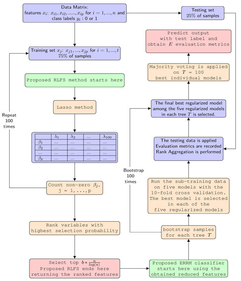
Figure 1.
The complete workflow depicting the proposed combination of RLFS-ERRM framework.
| Algorithm 1 Proposed ERRM |
|
2.5. Evaluation Metrics
We evaluated the results of combinations of FS methods with the classifier using accuracy and geometric mean (Gmean). The metrics are detailed with respect to true positive (TP), true negative (TN), false negative (FN), and false positive (FP). The equations for accuracy and Gmean are as follows:
where the sensitivity and specificity are given by:
3. Results
3.1. Simulation Results
The prediction performance of any given model is largely dependent on the type of the features. The features affecting the classification will help in attaining the best prediction accuracies. In Figure 2, we see the RLFS method with the top-ranked features based on the b-SIS criterion includes a higher number of true important features than other existing FS methods, such as IG, Chi2, and MRMR used for comparison in this study. The proposed RLFS performs consistently better across low, medium, and highly correlated simulated data, and the positive effect of having more true important variables was seen in all three simulation scenarios (further explained in detail).
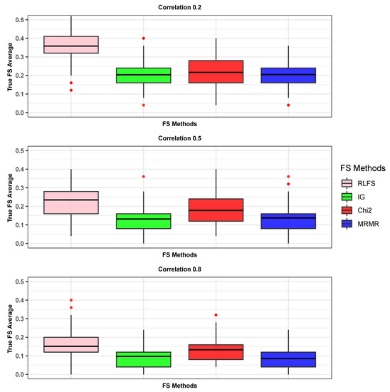
Figure 2.
True number of features selected among top b-SIS ranked features, and the average of this taken over 100 iterations for three different scenarios. The first horizontal line in the box shows the first quartile and the second horizontal dark line which usually represents the median values are shown as the mean values in this article. The third horizontal line in each of the boxes shows the third quartile. The red dotted circles indicate the outliers in each of the FS methods.
3.1.1. Simulation Scenario (S1): Low Correlation 0.2
The predictors were generated, having a low correlation structure with = 0.2. The proposed classifier ERRM performs better than the existing classifier on all the FS methods: proposed RLFS, IG, Chi2, and MRMR. Also, the proposed combination of ERRM classifier with RLFS method, with the accuracy and Gmean, each of which is 0.8606 and 0.8626 respectively, is relatively better in comparison to other combinations of FS method and classifier such as RLFS-LASSO, RLFS-ALASSO, RLFS-ENET, and the other remaining combinations, as observed in Figure 3. The combination of the FS method IG with proposed ERRM with an accuracy of 0.8476 is also seen performing better than IG-LASSO, IG-ALASSO, IG-ENET, IG-SCAD, IG-MCP, IG-AB, IG-RF, IG-LR, and IG-SVM. Similarly, the combination of Chi2-ERRM with an accuracy of 0.8538 is seen better than FS method Chi2 with the other remaining classifiers. The results are reported in Table 1. The combination of MRMR-ERRM has an accuracy of 0.8550 and Gmean of 0.8552 is better than the combination of FS method MRMR with the rest of the nine classifiers.
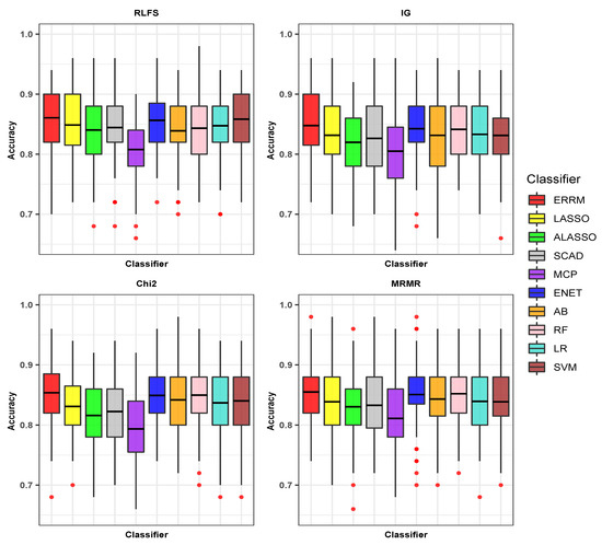
Figure 3.
Comparison of accuracies of proposed combination of ensemble of regularized regression models (ERRM) with resampling-based lasso feature selection (RLFS) and other classifiers with feature selection methods when correlation = 0.2.

Table 1.
Classification performance of proposed RLFS with ERRM compared to other combinations of feature selection methods with classifiers over 100 iterations.
All the classifiers with the features obtained from the RLFS method achieved the best accuracies in comparison to other FS methods, as seen in Figure 3. The combination of RLFS with SVM showed the second-best performance by attaining an accuracy of 0.8582, as seen in Table 1. The ENET method showed the best performance among all the regularized regression models with all the FS methods, and the best accuracy was obtained with the proposed RLFS method.
The proposed combination of RLFS-ERRM has better performance than the other existing combinations of the FS and classifier without the proposed FS method RLFS and classifier ERRM itself. For example, the existing FS methods IG, Chi2, and MRMR with the eight existing individual classifiers’ performances are lower than the proposed RLFS-ERRM combination, as shown in Table 1.
3.1.2. Simulation Scenario (S2): Intermediate Correlation 0.5
The predictor variables were generated using a medium correlation structure with = 0.5. The proposed combination of the RLFS method and ERRM classifier, with the accuracy and Gmean, each of which is 0.9256 and 0.9266, respectively, attained relatively better performance compared to other combinations of the FS method and classifier such as RLFS-LASSO, RLFS-ALASSO, RLFS-ENET and the other remaining combinations. The results are shown in Table 1. From Figure 4, we see that the proposed ensemble classifier ERRM with other FS methods such as IG, Chi2, and MRMR performs best compared to the other nine individual classifiers.
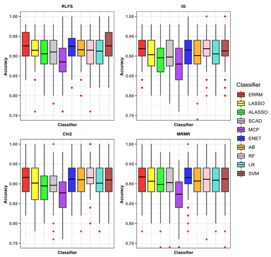
Figure 4.
Boxplot showing the accuracies of classifiers with FS methods when correlation = 0.5.
The SVM and ENET classifiers with the RLFS method attained accuracies that are almost similar to the proposed combination of ERRM-RLFS. However, when Gmean is considered, the ERRM-RLFS outperforms the SVM combinations. The average SD of the proposed combination of the ERRM-RLFS is smaller than other combinations of the FS method and classifier. The accuracies of SVM and ENET classifiers with the IG method were 0.9128 and 0.9150 lower compared to the ERRM classifier with the IG method which had an accuracy of 0.9184. Similarly, the ERRM with the Chi2 method showed relatively better performance than the competitive classifiers ENET and SVM. Further, the ERRM classifier with the MRMR method having an accuracy of 0.9174 showed better performance than ENET, SVM, and other top-performing individual classifiers.
While the SVM and ENET classifiers showed promising performance on the RLFS that had a good number of important features, they failed to show the same consistency on the other FS methods. On the other hand, the ensemble ERRM showed robust behavior, with being able to withstand the noise that helps in attaining better prediction accuracies and Gmean, not only with the RLFS method but also with other FS methods, such as IG, Chi2, and MRMR, as seen in Table 1.
Similar results are also found in the Simulation Scenario (S3): which has the highly correlated data with set to 0.8. The results for this scenario are described in the Appendix A.
3.2. Experimental Results
Figure 5 shows the box plot of average accuracies taken over 100 iterations for all the combinations of FS and classifiers in experimental data. Each of the sub-figures in the figure shows the classifiers with the corresponding FS methods. As seen in Table 2, the performance of all the individual classifiers when applied on the RLFS method—the accuracy and Gmean—are relatively much better than the accuracies of the individual classifiers when applied on the IG, Chi2, and MRMR methods.
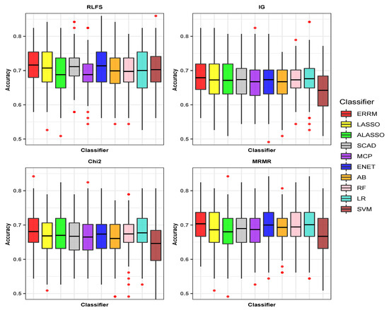
Figure 5.
Boxplot showing the accuracies of classifiers with FS methods in experimental data SMK-CAN-187.
Table 2.
Average values taken over 100 iterations in experimental data: SMK-CAN-187.
When we look at the performances of all the classifiers with the IG method in comparison to other FS methods, there is much variation in the accuracies, as seen in Figure 5. The SVM classifier, which attained the accuracy of 0.7026 with the RLFS method, dropped to 0.6422 with the IG method.
The proposed combination of the ERRM classifier with the RLFS method achieved the highest average accuracy of 0.7161, and the Gmean of 0.7127 outperformed the rest of the combinations of classifier with the FS method. The RLFS method is also a top-performing FS method on all individual classifiers. However, among the other FS methods, the MRMR method, when applied to all the individual classifiers, showed relatively much better performance than the application of IG and Chi2 methods to the individual classifiers. The second best-performing method is the ENET-RLFS combination, which had an accuracy of 0.7138. The SVM-IG combination showed the lowest performance with an accuracy of 0.6422 among all the combinations of the classifier with FS methods, as shown in Table 2.
For assessing the importance of bootstrapping and FS screening of the proposed framework, we measured the performance of ERRM without FS screening. The results in Table 3 shows the results of ensembles method with and without bootstrapping procedure. We see that having the bootstrapping approach which is random sampling with replacement is a better approach in the ensembles.
Table 3.
Comparison of proposed ERRM with and without bootstrapping.
The performance of the regularized regression models used in the proposed ensembles algorithm is tested with the FS screening method and without the FS screening method. In the former approach, the regularized regression models were built and tested using the proposed RLFS screening method with the selected amount of significant features, whereas in the latter approach, the regularized models used all the features for building the model. The performances of the penalized models with the FS screening showed better accuracies and Gmean than without FS screening, as reported in Table 4.
Table 4.
Comparison of regularized regression models used in the ERRM with and without FS screening.
4. Discussion
We investigated the performance of the proposed combination of ERRM with the RLFS method using simulation studies and a real data application. The RLFS method ranks the features by employing the lasso method with a resampling approach and the b-SIS criteria to set the threshold for selecting the optimal number of features, and these features are applied on the ERRM classifier, which uses bootstrapping and rank aggregation to select the best performing model across the bootstrapped samples and helps in attaining the best prediction accuracy in a high dimensional setting. The ensemble framework ERRM was built using five different regularized regression models. The regularized regression models are known for having the best performances in terms of variable selection and prediction accuracy on gene expression data.
To show the performance of our proposed framework, we used three different simulation scenarios with low, medium, and high correlation structures that matched the gene expression data. To further illustrate our point, we also used SMK-CAN-187 data. Figure 2 shows the boxplots of the average number of true important features, where the RLFS shows higher detection power than the other FS methods such as IG, Chi2, and MRMR. From the results of both simulation studies and experimental data, we showed that all the individual classifiers with the RLFS method performed much better compared to the IG, Chi2, and MRMR. We also observed that all the individual classifiers showed much instability with the other three FS methods. This means that the individual classifiers do not work well with more noise and less true important variables in the model. The SVM and ENET classifiers with all the FS methods performed a little better among all the classifiers. However, the performance was relatively still low in comparison to the proposed ERRM classifier with every FS method. The tree-based ensemble methods RF and AB with RLFS also attained good accuracies but were not the best compared to the ERRM classifier.
The proposed ERRM method was assessed with the FS screening and without the FS screening step along with the bootstrapping option. The ERRM with FS screening and bootstrapping approach works better than ERRM without the FS screening and bootstrapping technique. Also, the results from Table 3 show that the ensemble with bootstrapping is a better approach to both the filtered and unfiltered data. On comparing the performance of the individual regularized regression models used in the ensembles, the individual models with the proposed RLFS screening step showed comparatively better accuracy in comparison to the individual regularized regression models without the FS screening. This means that using the reduced number of significant features with RLFS is a better approach instead of using all the features from the data.
The importance of FS method was not addressed in any of the ensemble approaches [37,38,39], and the classification accuracies achieved by the corresponding proposed methods were much closer to the accuracies attained by existing approaches. In this paper, we compared the various combination of FS methods with different classifiers. The ERRM showed better overall performance not only with the RLFS but also with the other FS methods compared in this study. This means that the ERRM is robust and works much better on the highly correlated gene expression data. The rule of thumb fpr attaining the best prediction accuracy is that more the true important variables, better the prediction accuracy. Henceforth, from the results of simulation and experimental data, we see that the proposed combination of RLFS-ERRM is better compared to the other existing combinations of FS and classifiers, as seen in the Table 1 and Table 2. The proposed ERRM classifier showed the best performance across all the FS methods, with the highest performance achieved with the RLFS method. The proposed RLFS method attained a higher number of significant features compared to other FS methods. However, the drawback is that with the increase in the correlation structure, there is a decreasing performance in selecting the significant features, as shown in Figure 2. The ensembles algorithms are known to be computationally expensive [39] because of the tree-based nature. However, in our proposed framework, before the ensembles of ERRM, we apply FS methods to remove the irrelevant features and keep significant features. This filtering step not only helps with improving prediction accuracy but also with overcoming the drawback of computational time required, as the number of features processed becomes lower.
5. Conclusions
In this paper, we proposed a combination of the ensembles of regularized regression models (ERRM) with resampling-based lasso feature selection (RLFS) for attaining better prediction accuracies in high dimensional data. We conducted extensive simulation studies where we showed the better performance of RLFS in detecting the significant features than other competitive FS methods. The ensemble classifier ERRM also showed better average prediction accuracy with the RLFS, IG, Chi2, and MRMR compared to other classifiers with these FS methods. We also saw an improved performance in the ensemble method when used with bootstrapping. On comparing the performances of individual regularized regression models, all the models showed an increase in their accuracies with the FS screening approach. In both the simulation study and the experimental data SMK-CAN-187, the better performance was achieved by the proposed combination of RLFS and ERRM compared to all other combinations of FS and classifiers. The minor drawback in the proposed framework is that, in the case of highly correlated data, there is smaller number of significant features selected with all the FS methods. As future work, we plan to focus on improving the detecting power of true important genes with the new FS method.
Author Contributions
Conceptualization, S.K. and A.R.P.; formal analysis and investigation, A.R.P.; writing—original draft preparation, A.R.P.; supervision and reviewing, S.K. All authors have read and agreed to the published version of the manuscript.
Funding
This research received no external funding.
Acknowledgments
We would like to thank the editors and three anonymous reviewers for their insightful comments and helpful suggestions.
Conflicts of Interest
The authors declare no conflict of interest.
Abbreviations
The following abbreviations are used in this manuscript:
| FS | feature Selection |
| RLFS | resampling-based lasso feature selection |
| ERRM | ensemble regularized regression models |
| IG | information gain |
| Chi2 | chi-square |
| MRMR | minimum redundancy maximum relevance |
| ALASSO | adaptive lasso |
| AB | adaptive boosting |
| RF | random forests |
| LR | logistic regression |
| SVM | support vector machines |
| SD | standard deviation |
Appendix A
The data are generated based on a high correlation data structure with = 0.8. The performance of the proposed combination of RLFS-ERRM is relatively better than the other combinations of the FS methods and classifiers. The results for simulation scenario S3 are shown in Figure A1. The average accuracies and Gmeans for all the FS and classifiers are noted in Table A1. The SVM and ENET classifiers with all the FS methods showed a little better performance among all individual classifiers. However, the accuracies and Gmeans attained by the proposed ensemble classifier ERRM with the FS methods RLFS, IG, and Chi2 were relatively better compared to the individual classifiers with FS methods. The best performance was achieved by the proposed RLFS-ERRM combination with an accuracy of 0.9586 and Gmean of 0.9596. The second-best performing combination was MRMR-SVM. The lowest performance in terms of accuracy and the Gmean was shown by Chi2-MCP. The MCP classifier has the lowest accuracy with all the FS methods. This explains why the MCP does not perform well when the predictor variables are highly correlated.

Figure A1.
Boxplot showing the accuracies of Classifiers with FS methods in simulation scenario: S3 (Correlation = 0.8).
Figure A1.
Boxplot showing the accuracies of Classifiers with FS methods in simulation scenario: S3 (Correlation = 0.8).

Table A1.
Average values taken over 100 iterations in simulation scenario: S3 (High correlation: 0.8).
Table A1.
Average values taken over 100 iterations in simulation scenario: S3 (High correlation: 0.8).
| Proposed RLFS | IG | Chi2 | MRMR | |||||
|---|---|---|---|---|---|---|---|---|
| Classifier | Accuracy (SD) | Gmean (SD) | Accuracy (SD) | Gmean (SD) | Accuracy (SD) | Gmean (SD) | Accuracy (SD) | Gmean (SD) |
| Proposed ERRM | 0.9586 (0.025) | 0.9596 (0.039) | 0.9556 (0.027) | 0.9565 (0.041) | 0.9530 (0.034) | 0.9544 (0.045) | 0.9560 (0.024) | 0.9558 (0.037) |
| LASSO | 0.9482 (0.033) | 0.9493 (0.050) | 0.9442 (0.030) | 0.9194 (0.045) | 0.9428 (0.037) | 0.9447 (0.051) | 0.9444 (0.032) | 0.9442 (0.042) |
| ALASSO | 0.9420 (0.031) | 0.9425 (0.051) | 0.9376 (0.030) | 0.9379 (0.045) | 0.9328 (0.041) | 0.942 (0.056) | 0.9388 (0.033) | 0.9389 (0.047) |
| ENET | 0.9576 (0.025) | 0.9587 (0.039) | 0.9538 (0.029) | 0.9546 (0.042) | 0.9532 (0.034) | 0.9546 (0.045) | 0.9566 (0.024) | 0.9562 (0.036) |
| SCAD | 0.9464 (0.031) | 0.9475 (0.049) | 0.9422 (0.030) | 0.9428 (0.045) | 0.9386 (0.043) | 0.9401 (0.055) | 0.9414 (0.031) | 0.9408 (0.043) |
| MCP | 0.9256 (0.040) | 0.9270 (0.062) | 0.9262 (0.038) | 0.9269 (0.055) | 0.9210 (0.041) | 0.9221 (0.058) | 0.9224 (0.034) | 0.9223 (0.048) |
| AB | 0.9454 (0.032) | 0.9469 (0.047) | 0.9494 (0.030) | 0.9501 (0.044) | 0.9470 (0.034) | 0.9482 (0.046) | 0.9480 (0.029) | 0.9481 (0.040) |
| RF | 0.9540 (0.030) | 0.9557 (0.043) | 0.9560 (0.029) | 0.9565 (0.043) | 0.9542 (0.032) | 0.9556 (0.044) | 0.9508 (0.027) | 0.9510 (0.039) |
| LR | 0.9478 (0.029) | 0.9482 (0.045) | 0.9462 (0.030) | 0.9469 (0.044) | 0.9418 (0.038) | 0.9432 (0.050) | 0.9438 (0.028) | 0.9437 (0.041) |
| SVM | 0.9560 (0.027) | 0.9568 (0.041) | 0.9522 (0.030) | 0.9527 (0.043) | 0.9520 (0.031) | 0.9526 (0.042) | 0.9594 (0.026) | 0.9587 (0.037) |
References
- Tariq, H.; Eldridge, E.; Welch, I. An efficient approach for feature construction of high-dimensional microarray data by random projections. PLoS ONE 2018, 13, e0196385. [Google Scholar] [CrossRef] [PubMed]
- Bhola, A.; Singh, S. Gene Selection Using High Dimensional Gene Expression Data: An Appraisal. Curr. Bioinform. 2018, 13, 225–233. [Google Scholar] [CrossRef]
- Dai, J.J.; Lieu, L.H.; Rocke, D.M. Dimension reduction for classification with gene expression microarray data. Stat. Appl. Genet. Mol. Biol. 2006, 5, 6. [Google Scholar] [CrossRef] [PubMed]
- Lu, J.; Kerns, R.T.; Peddada, S.D.; Bushel, P.R. Principal component analysis-based filtering improves detection for Affymetrix gene expression arrays. Nucleic Acids Res. 2011, 39, e86. [Google Scholar] [CrossRef]
- Bourgon, R.; Gentleman, R.; Huber, W. Reply to Talloen et al.: Independent filtering is a generic approach that needs domain specific adaptation. Proc. Natl. Acad. Sci. USA 2010, 107, E175. [Google Scholar] [CrossRef]
- Bourgon, R.; Gentleman, R.; Huber, W. Independent filtering increases detection power for high-throughput experiments. Proc. Natl. Acad. Sci. USA 2010, 107, 9546–9551. [Google Scholar] [CrossRef]
- Ramsköld, D.; Wang, E.T.; Burge, C.B.; Sandberg, R. An Abundance of Ubiquitously Expressed Genes Revealed by Tissue Transcriptome Sequence Data. PLoS Comput. Biol. 2009, 5, e1000598. [Google Scholar] [CrossRef]
- Li, L.; Kabesch, M.; Bouzigon, E.; Demenais, F.; Farrall, M.; Moffatt, M.; Lin, X.; Liang, L. Using eQTL weights to improve power for genome-wide association studies: A genetic study of childhood asthma. Front. Genet. 2013, 4, 103. [Google Scholar] [CrossRef]
- Calle, M.L.; Urrea, V.; Vellalta, G.; Malats, N.; Steen, K.V. Improving strategies for detecting genetic patterns of disease susceptibility in association studies. Stat. Med. 2008, 27, 6532–6546. [Google Scholar] [CrossRef]
- Bock, C. Analysing and interpreting DNA methylation data. Nat. Rev. Genet. 2012, 13, 705–719. [Google Scholar] [CrossRef]
- Sun, H.; Wang, S. Penalized logistic regression for high-dimensional DNA methylation data with case-control studies. Bioinformatics 2012, 28, 1368–1375. [Google Scholar] [CrossRef]
- Kim, S.; Halabi, S. High Dimensional Variable Selection with Error Control. BioMed Res. Int. 2016, 2016, 8209453. [Google Scholar] [CrossRef] [PubMed]
- Kim, S.; Kim, J.M. Two-Stage Classification with SIS Using a New Filter Ranking Method in High Throughput Data. Mathematics 2019, 7, 493. [Google Scholar] [CrossRef]
- Fan, J.; Lv, J. Sure independence screening for ultrahigh dimensional feature space. J. R. Stat. Soc. Ser. B 2008, 70, 849–911. [Google Scholar] [CrossRef] [PubMed]
- Quinlan, J.R. C4.5: Programs for Machine Learning; Morgan Kaufmann Publishers Inc.: San Francisco, CA, USA, 1993. [Google Scholar]
- Okeh, U.; Oyeka, I. Estimating the Fisher’s Scoring Matrix Formula from Logistic Model. Am. J. Theor. Appl. Stat. 2013, 2013, 221–227. [Google Scholar]
- Guyon, I.; Elisseeff, A. An Introduction to Variable and Feature Selection. J. Mach. Learn. Res. 2003, 3, 1157–1182. [Google Scholar]
- Peng, H.; Long, F.; Ding, C. Feature Selection Based on Mutual Information: Criteria of Max-Dependency, Max-Relevance, and Min-Redundancy. IEEE Trans. Pattern Anal. Mach. Intell. 2005, 27, 1226–1238. [Google Scholar] [CrossRef]
- Ditzler, G.; Morrison, J.C.; Lan, Y.; Rosen, G.L. Fizzy: Feature subset selection for metagenomics. BMC Bioinform. 2015, 16, 358. [Google Scholar] [CrossRef]
- Su, C.T.; Yang, C.H. Feature selection for the SVM: An application to hypertension diagnosis. Expert Syst. Appl. 2008, 34, 754–763. [Google Scholar] [CrossRef]
- Kursa, M.B.; Rudnicki, W.R. Feature Selection with the Boruta Package. 2010. [Google Scholar]
- Urbanowicz, R.J.; Meeker, M.; Cava, W.L.; Olson, R.S.; Moore, J.H. Relief-based feature selection: Introduction and review. J. Biomed. Inform. 2017, 85, 189–203. [Google Scholar] [CrossRef] [PubMed]
- Breiman, L. Random Forests. Mach. Learn. 2001, 45, 5–32. [Google Scholar] [CrossRef]
- Freund, Y. An Adaptive Version of the Boost by Majority Algorithm. Mach. Learn. 2001, 43, 293–318. [Google Scholar] [CrossRef]
- Hearst, M.A.; Dumais, S.T.; Osuna, E.; Platt, J.; Scholkopf, B. Support vector machines. IEEE Intell. Syst. Appl. 1998, 13, 18–28. [Google Scholar] [CrossRef]
- Statnikov, A.R.; Wang, L.; Aliferis, C.F. A comprehensive comparison of random forests and support vector machines for microarray-based cancer classification. BMC Bioinform. 2008, 9, 319. [Google Scholar] [CrossRef] [PubMed]
- Tibshirani, R. Regression Shrinkage and Selection via the Lasso. J. R. Stat. Soc. Ser. B (Methodol.) 1996, 58, 267–288. [Google Scholar] [CrossRef]
- Marquardt, D.W.; Snee, R.D. Ridge Regression in Practice. Am. Stat. 1975, 29, 3–20. [Google Scholar]
- Yang, X.G.; Lu, Y. Informative Gene Selection for Microarray Classification via Adaptive Elastic Net with Conditional Mutual Information. arXiv 2018, arXiv:1806.01466. [Google Scholar]
- Fan, J.; Li, R. Variable Selection via Nonconcave Penalized Likelihood and its Oracle Properties. J. Am. Stat. Assoc. 2001, 96, 1348–1360. [Google Scholar] [CrossRef]
- Zhang, C.H. Nearly unbiased variable selection under minimax concave penalty. Ann. Stat. 2010, 38, 894–942. [Google Scholar] [CrossRef]
- Hastie, T.; Tibshirani, R.; Friedman, J. The Elements of Statistical Learning: Data Mining, Inference And Prediction, 2nd ed.; Springer: Berlin/Heidelberg, Germany, 2009. [Google Scholar]
- Dietterich, T.G. Ensemble Methods in Machine Learning. In International Workshop on Multiple Classifier Systems; Springer: London, UK, 2000; pp. 1–15. [Google Scholar]
- Maclin, R.; Opitz, D.W. Popular Ensemble Methods: An Empirical Study. arXiv 2011, arXiv:1106.0257. [Google Scholar]
- Breiman, L. Bagging Predictors. Mach. Learn. 1996, 24, 123–140. [Google Scholar] [CrossRef]
- Freund, Y.; Schapire, R.E. A Decision-Theoretic Generalization of On-Line Learning and an Application to Boosting. J. Comput. Syst. Sci. 1997, 55, 119–139. [Google Scholar] [CrossRef]
- Datta, S.; Pihur, V.; Datta, S. An adaptive optimal ensemble classifier via bagging and rank aggregation with applications to high dimensional data. BMC Bioinform. 2010, 11, 427. [Google Scholar] [CrossRef] [PubMed]
- Ahn, H.; Moon, H.; Fazzari, M.J.; Lim, N.; Chen, J.J.; Kodell, R.L. Classification by ensembles from random partitions of high-dimensional data. Comput. Stat. Data Anal. 2007, 51, 6166–6179. [Google Scholar] [CrossRef]
- Lim, N.; Ahn, H.; Moon, H.; Chen, J.J. Classification of high-dimensional data with ensemble of logistic regression models. J. Biopharm. Stat. 2009, 20, 160–171. [Google Scholar] [CrossRef]
- R Development Core Team. R: A Language and Environment for Statistical Computing; R Foundation for Statistical Computing: Vienna, Austria, 2008; ISBN 3-900051-07-0. [Google Scholar]
- Kursa, M.B. Praznik: Collection of Information-Based Feature Selection Filters; R Package Version 5.0.0; R Foundation for Statistical Computing: Vienna, Austria, 2018. [Google Scholar]
- Novoselova, N.; Wang, J.; F.P.F.K. Biocomb: Feature Selection and Classification with the Embedded Validation Procedures for Biomedical Data Analysis, R package version 0.4; R Foundation for Statistical Computing: Vienna, Austria, 2018. [Google Scholar]
- Friedman, J.; Hastie, T.; Tibshirani, R. Regularization Paths for Generalized Linear Models via Coordinate Descent. J. Stat. Softw. 2010, 33, 1–22. [Google Scholar] [CrossRef]
- Breheny, P.; Huang, J. Coordinate descent algorithms for nonconvex penalized regression, with applications to biological feature selection. Ann. Appl. Stat. 2011, 5, 232–253. [Google Scholar] [CrossRef]
- Liaw, A.; Wiener, M. Classification and Regression by randomForest. R News 2002, 2, 18–22. [Google Scholar]
- Meyer, D.; Dimitriadou, E.; Hornik, K.; Weingessel, A.; Leisch, F. e1071: Misc Functions of the Department of Statistics, Probability Theory Group (Formerly: E1071), TU Wien; R Package Version 1.7-1; R Foundation for Statistical Computing: Vienna, Austria, 2019. [Google Scholar]
- Pihur, V.; Datta, S.; Datta, S. RankAggreg: Weighted Rank Aggregation, R package version 0.6.5; R Foundation for Statistical Computing: Vienna, Austria, 2018. [Google Scholar]
- The RLFS-ERRM Resources 2019. Available online: https://sites.google.com/site/abhijeetrpatil01/file-cabinet/blfs-errm-manuscript-files-2019 (accessed on 25 December 2019).
- Feature Selection Datasets. Available online: http://featureselection.asu.edu/old/datasets.php (accessed on 25 December 2019).
- Bolón-Canedo, V.; Sánchez-Maroño, N.; Alonso-Betanzos, A.; Benítez, J.M.; Herrera, F. A review of microarray datasets and applied feature selection methods. Inf. Sci. 2014, 282, 111–135. [Google Scholar] [CrossRef]
- Wang, M.; Barbu, A. Are screening methods useful in feature selection? An empirical study. PLoS ONE 2018, 14, e0220842. [Google Scholar] [CrossRef]
- Tsai, C.; Chen, J.J. Multivariate analysis of variance test for gene set analysis. Bioinformatics 2009, 25, 897–903. [Google Scholar] [CrossRef] [PubMed]
- Li, J.; Cheng, K.; Wang, S.; Morstatter, F.; Trevino, R.P.; Tang, J.; Liu, H. Feature Selection: A Data Perspective. ACM Comput. Surv. 2017, 50, 94:1–94:45. [Google Scholar] [CrossRef]
- Chen, X.D.; Ishwaran, H. Random forests for genomic data analysis. Genomics 2012, 99, 323–329. [Google Scholar] [CrossRef] [PubMed]
- Bielza, C.; Robles, V.; Larrañaga, P. Regularized logistic regression without a penalty term: An application to cancer classification with microarray data. Expert Syst. Appl. 2011, 38, 5110–5118. [Google Scholar] [CrossRef]
- Liao, J.G.; Chin, K.V. Logistic regression for disease classification using microarray data: model selection in a large p and small n case. Bioinformatics 2007, 23, 1945–1951. [Google Scholar] [CrossRef] [PubMed]
- Zou, H.; Hastie, T. Regularization and Variable Selection via the Elastic Net. J. R. Stat. Soc. Ser. B (Stat. Methodol.) 2005, 67, 301–320. [Google Scholar] [CrossRef]
- Li, Y.; Zhang, Y.; Zhao, S. Gender Classification with Support Vector Machines Based on Non-tensor Pre-wavelets. In Proceedings of the 2010 Second International Conference on Computer Research and Development, Kuala Lumpur, Malaysia, 7–10 May 2010; pp. 770–774. [Google Scholar]


© 2020 by the authors. Licensee MDPI, Basel, Switzerland. This article is an open access article distributed under the terms and conditions of the Creative Commons Attribution (CC BY) license (http://creativecommons.org/licenses/by/4.0/).