Variational Partitioned Runge–Kutta Methods for Lagrangians Linear in Velocities

Abstract

In this paper, we construct higher-order variational integrators for a class of degenerate systems described by Lagrangians that are linear in velocities. We analyze the geometry underlying such systems and develop the appropriate theory for variational integration. Our main observation is that the evolution takes place on the primary constraint and the “Hamiltonian” equations of motion can be formulated as an index-1 differential-algebraic system. We also construct variational Runge–Kutta methods and analyze their properties. The general properties of Runge–Kutta methods depend on the “velocity” part of the Lagrangian. If the “velocity” part is also linear in the position coordinate, then we show that non-partitioned variational Runge–Kutta methods are equivalent to integration of the corresponding first-order Euler–Lagrange equations, which have the form of a Poisson system with a constant structure matrix, and the classical properties of the Runge–Kutta method are retained. If the “velocity” part is nonlinear in the position coordinate, we observe a reduction of the order of convergence, which is typical of numerical integration of DAEs. We verified our results through numerical experiments for various dynamical systems.

1. Introduction

Geometric integrators are numerical methods that preserve geometric structures and properties of the flow of a differential equation. Structure-preserving integrators have attracted considerable interest due to their excellent numerical behavior, especially for long-time integration of equations possessing geometric properties (see [1,2,3]).

An important class of structure-preserving integrators are variational integrators. This type of numerical schemes is based on discrete variational principles and provides a natural framework for the discretization of Lagrangian systems, including forced, dissipative, constrained, or stochastic ones. For an overview of variational integration, see [4] (see also [5,6,7,8,9,10,11,12,13,14,15,16,17,18]). Variational integrators were introduced in the context of finite-dimensional mechanical systems, but were later generalized to Lagrangian field theories (see [19]) and applied in many computations, for example in elasticity, electrodynamics, or fluid dynamics (see [20,21,22,23,24]).

Theoretical aspects of variational integration are well understood in the case when the Lagrangian describing the considered system is regular, that is, when the corresponding Legendre transform is (at least locally) invertible. However, the corresponding theory for degenerate Lagrangian systems is less developed. The analysis of degenerate systems becomes more cumbersome, because the Euler–Lagrange equations may cease to be second order, or may not even make any sense at all. In the latter case, one needs to determine if there exists a submanifold of the configuration bundle $TQ$ on which consistent equations of motion can be derived. This can be accomplished by applying the Dirac theory of constraints or the pre-symplectic constraint algorithm (see [25,26]).

A particularly simple case of degeneracy occurs when the Lagrangian is linear in velocities. In that case, the dynamics of the system is defined on the configuration manifold Q itself, rather than its tangent bundle $TQ$, provided that some regularity conditions are satisfied. Such systems arise in many physical applications, including interacting point vortices in the plane (see [17,18,27]), guiding center dynamics (see [28,29,30,31,32]), or partial differential equations such as the nonlinear Schrödinger [33], KdV [34,35] or Camassa–Holm equations [36,37]. In Section 5, we show how certain Poisson systems can be recast as Lagrangian systems whose Lagrangians are linear in velocities. Therefore, our approach offers a new perspective on geometric integration of Poisson systems, which often arise as semi-discretizations of integrable nonlinear partial differential equations, e.g., the Toda or Volterra lattice equations, and play an important role in the modeling of many physical phenomena (see [38,39,40]).

This paper is organized as follows. In Section 2, we introduce a proper geometric setup and discuss the properties of systems that are linear in velocities. In Section 3, we analyze the general properties of variational integrators and point out how the relevant theory differs from the non-degenerate case. In Section 4, we introduce variational partitioned Runge–Kutta methods and discuss their relation to numerical integration of differential-algebraic systems. In Section 5, we present the results of our numerical experiments for Kepler’s problem, a system of two interacting vortices, and the Lotka–Volterra model. We summarize our work and discuss possible extensions in Section 6.

2. Geometric Setup

Let Q be the configuration manifold and $TQ$ its tangent bundle. Throughout this work, we assume that the dimension of the configuration manifold $dimQ=n$ is even. We further assume Q is a vector space and by a slight abuse of notation we denote by q both an element of Q and the vector of its coordinates $q=(q^1,\dots ,q^n)$ in a local chart on Q. It is clear from the context which definition is invoked. Consider the Lagrangian $L:TQ⟶\mathbb{R}$ given by

$$L(v_q)=⟨\alpha ,v_q⟩-H(q),$$

(1)

where $\alpha :Q⟶T^{*}Q$ is a smooth one-form, $H:Q⟶\mathbb{R}$ is the Hamiltonian, and $v_q\in T_{q}Q$. Let $(q^{\mu },{\dot{q}}^{\mu })$ denote canonical coordinates on $TQ$, where $\mu =1,\dots ,n$. In these coordinates, we can consider

$$L(q,\dot{q})={\alpha }_{\mu }(q){\dot{q}}^{\mu }-H(q),$$

(2)

where summation over repeated Greek indices is implied.

2.1. Equations of Motion

The Lagrangian in Equation (1) is degenerate, since the associated Legendre transform

$$\mathbb{F}L:TQ\ni v_q⟶{\alpha }_q\in T^{*}Q$$

(3)

is not invertible. The local representation of the Legendre transform is

$$\begin{array}{c}\hfill \mathbb{F}L(q^{\mu },{\dot{q}}^{\mu })=\left(q^{\mu },\frac{\partial L}{\partial {\dot{q}}^{\mu }}\right)=\left(q^{\mu },{\alpha }_{\mu }(q)\right),\end{array}$$

(4)

that is,

$$p_{\mu }={\alpha }_{\mu }(q),$$

(5)

where $(q^{\mu },p_{\mu })$ denote canonical coordinates on $T^{*}Q$. The dynamics is defined by the action functional

$$S\left[q(t)\right]={\int }_a^{b}L\left(q(t),\dot{q}(t)\right)dt$$

(6)

and Hamilton’s principle, which seeks the curves $q(t)$ such that the functional $S[q(t)]$ is stationary under variations of $q(t)$ with fixed endpoints, i.e., we seek $q(t)$ such that

$$\begin{array}{c}\hfill dS\left[q(t)\right]·\delta q(t)=\frac{d}{dϵ}{|}_{ϵ=0}S\left[q_{ϵ}(t)\right]=0\end{array}$$

(7)

for all $\delta q(t)$ with $\delta q(a)=\delta q(b)=0$, where $q_{ϵ}(t)$ is a smooth family of curves satisfying $q_0=q$ and $\frac{d}{dϵ}{|}_{ϵ=0}{q}_{ϵ}=\delta q$. The resulting Euler–Lagrange equations

$$M_{\mu \nu }(q){\dot{q}}^{\nu }={\partial }_{\mu }H(q)$$

(8)

form a system of first-order ODEs, where we assume that the even-dimensional antisymmetric matrix $M_{\mu \nu }(q)={\partial }_{\mu }{\alpha }_{\nu }(q)-{\partial }_{\nu }{\alpha }_{\mu }(q)$ is invertible for all $q\in Q$. Without loss of generality, we can further assume that the coordinate mapping $p_{\mu }={\alpha }_{\mu }(q)$ is invertible and its inverse is smooth: if the Jacobian $\partial {\alpha }_{\mu }/\partial q^{\nu }$ is singular, we can redefine ${\alpha }_{\mu }(q)\to {\alpha }_{\mu }(q)+b_{\mu }(q^{\mu })$, where $b_{\mu }(q^{\mu })$ are arbitrary functions; the Euler–Lagrange equations remain the same, and with the right choice of the functions $b_{\mu }(q^{\mu })$, the redefined Jacobian can be made nonsingular. Using $B=M^{-1}$, Equation (8) can be equivalently written as the Poisson system

$${\dot{q}}^{\mu }=B^{\mu \nu }(q){\partial }_{\nu }H(q).$$

(9)

The Euler–Lagrange Equation (8) can also be formulated as the implicit “Hamiltonian” system

$$\begin{array}{cc}\hfill p_{\mu }& ={\alpha }_{\mu }(q),\hfill \\ \hfill {\dot{p}}_{\mu }& ={\partial }_{\mu }{\alpha }_{\nu }(q){\dot{q}}^{\nu }-{\partial }_{\mu }H(q).\hfill \end{array}$$

(10)

Since the Lagrangian L is degenerate, Equation (10) is an index-1 system of differential-algebraic equations (DAE), rather than a Hamiltonian ODE system: the Legendre transform is an algebraic equation and has to be differentiated once with respect to time in order to turn this system into Equation (8). This reflects the fact that the evolution of the considered degenerate system takes place on the primary constraint$N=\mathbb{F}L(TQ)⊊T^{*}Q$. It is easy to see that the primary constraint N is (locally) diffeomorphic to the configuration manifold Q, where the diffeomorphism $\eta :Q\ni q⟶{\alpha }_q\in N$ is locally, in the coordinates on $T^{*}Q$, given by

$$\eta (q)=(q,\alpha (q)),$$

(11)

where by a slight abuse of notation $\alpha (q)=({\alpha }_1(q),\dots ,{\alpha }_n(q))$. This shows that $q^{\mu }$ can also be used as local coordinates on N. Note that $\eta$ is simply the restriction of $\alpha$ to N, i.e., ${\eta =\alpha |}_{Q⟶N}$.

2.2. Symplectic Forms

The spaces Q, $TQ$, $T^{*}Q$ and N can be equipped with several symplectic or pre-symplectic forms. It is instructive to investigate the relationships among them in order to later avoid confusion regarding the sense in which variational integrators for Lagrangians linear in velocities are symplectic. On the configuration space Q, we can define the two-form

$$\Omega =-d\alpha ,$$

(12)

which in local coordinates can be expressed as

$$\Omega =-d{\alpha }_{\mu }\wedge d{q}^{\mu }=-M_{\mu \nu }(q)d{q}^{\mu }\otimes d{q}^{\nu }.$$

(13)

The two-form $\Omega$ is symplectic if it is nondegenerate, i.e., if the matrix $M_{\mu \nu }$ is invertible for all q.

The cotangent bundle $T^{*}Q$ is equipped with the canonical Cartan one-form $\tilde{\mathsf{\Theta }}:T^{*}Q⟶T^{*}{T}^{*}Q$, which is intrinsically defined by the formula

$$\tilde{\mathsf{\Theta }}(\omega )={({\pi }_{T^{*}Q})}^{*}\omega$$

(14)

for any $\omega \in T^{*}Q$, where ${\pi }_{T^{*}Q}:T^{*}Q⟶Q$ is the cotangent bundle projection. In canonical coordinates, we have

$$\tilde{\mathsf{\Theta }}=p_{\mu }d{q}^{\mu }.$$

(15)

We further have the canonical symplectic two-form

$$\tilde{\Omega }=-d\tilde{\mathsf{\Theta }}=d{q}^{\mu }\wedge d{p}_{\mu }.$$

(16)

The symplectic forms $\Omega$ and $\tilde{\Omega }$ are related by

$$\Omega ={\alpha }^{*}\tilde{\Omega }.$$

(17)

This follows from the simple calculation

$${\alpha }^{*}\tilde{\mathsf{\Theta }}·v_q=\tilde{\mathsf{\Theta }}({\alpha }_q)·T\alpha (v_q)={\alpha }_q·T{\pi }_{T^{*}Q}\circ T\alpha (v_q)={\alpha }_q·T({\pi }_{T^{*}Q}\circ \alpha )(v_q)={\alpha }_q·v_q,$$

(18)

where we used Equation (14) and the fact that ${\pi }_{T^{*}Q}\circ \alpha ={\mathrm{id}}_Q$. Hence, ${\alpha }^{*}\tilde{\mathsf{\Theta }}=\alpha$, and taking the exterior derivative on both sides we obtain Equation (17).

Using the Legendre transform (Equation (3)) we can define the Lagrangian two-form ${\tilde{\Omega }}_L$ on $TQ$ by ${\tilde{\Omega }}_L=\mathbb{F}{L}^{*}\tilde{\Omega }$, which in canonical coordinates $(q^{\mu },{\dot{q}}^{\mu })$ is given by

$${\tilde{\Omega }}_L=d{q}^{\mu }\wedge d{\alpha }_{\mu }=-M_{\mu \nu }(q)d{q}^{\mu }\otimes d{q}^{\nu }.$$

(19)

The Lagrangian form ${\tilde{\Omega }}_L$ is only pre-symplectic, because it is degenerate. Noting that $\mathbb{F}L=\alpha \circ {\pi }_{TQ}$, where ${\pi }_{TQ}:TQ⟶Q$ is the tangent bundle projection, we can relate $\Omega$ and ${\tilde{\Omega }}_L$ through the formula

$${\tilde{\Omega }}_L={({\pi }_{TQ})}^{*}{\alpha }^{*}\tilde{\Omega }={({\pi }_{TQ})}^{*}\Omega .$$

(20)

The symplectic structure on N can be introduced in two ways: by pushing forward $\Omega$ from Q, or pulling back $\tilde{\Omega }$ from $T^{*}Q$. Both ways are equivalent, with

$${\tilde{\Omega }}_N={\eta }_{*}\Omega =i^{*}\tilde{\Omega },$$

(21)

where $i:N⟶T^{*}Q$ is the inclusion map. This follows from the calculation

$${\eta }_{*}\Omega ={({\eta }^{-1})}^{*}{\alpha }^{*}\tilde{\Omega }={(\alpha \circ {\eta }^{-1})}^{*}\tilde{\Omega }=i^{*}\tilde{\Omega },$$

(22)

where we used $\alpha =i\circ \eta$. If we use $q^{\mu }$ as coordinates on N, then the local representation of ${\tilde{\Omega }}_N$ is given by Equation (13).

2.3. Symplectic Flows

Let ${\phi }_t:Q⟶Q$ denote the flow of Equation (8) or Equation (9). This flow is symplectic on Q, that is

$${\phi }_t^{*}\Omega =\Omega .$$

(23)

This fact can be proven by considering the Hamiltonian or Poisson properties of Equation (8) or Equation (9) (see [1,26]). It also follows directly from the action principle in Equation (7) (see [17]).

Since the Lagrangian in Equation (1) is degenerate, the dynamics of the system is defined on Q rather than $TQ$. However, we can obtain the associated flow on $TQ$ through lifting ${\phi }_t$ by its tangent map $T{\phi }_t:TQ⟶TQ$. This flow preserves the Lagrangian two-form

$${(T{\phi }_t)}^{*}{\tilde{\Omega }}_L={\tilde{\Omega }}_L.$$

(24)

This can be seen from the calculation

$${(T{\phi }_t)}^{*}{\tilde{\Omega }}_L={(T{\phi }_t)}^{*}{({\pi }_{TQ})}^{*}\Omega ={({\pi }_{TQ}\circ T{\phi }_t)}^{*}\Omega ={({\phi }_t\circ {\pi }_{TQ})}^{*}\Omega ={({\pi }_{TQ})}^{*}{\phi }_t^{*}\Omega ={\tilde{\Omega }}_L,$$

(25)

where we use Equations (20) and (23), and the property ${\pi }_{TQ}\circ T{\phi }_t={\phi }_t\circ {\pi }_{TQ}$.

The flow ${\phi }_t$ induces the flow ${\tilde{\phi }}_t:N⟶N$ in a natural way as

$${\tilde{\phi }}_t=\eta \circ {\phi }_t\circ {\eta }^{-1}.$$

(26)

This flow is symplectic on N, i.e.,

$${\tilde{\phi }}_t^{*}{\tilde{\Omega }}_N={\tilde{\Omega }}_N,$$

(27)

which can be established through the simple calculation

$${\tilde{\phi }}_t^{*}{\tilde{\Omega }}_N={(\eta \circ {\phi }_t\circ {\eta }^{-1})}^{*}{\eta }_{*}\Omega ={({\eta }^{-1})}^{*}{\phi }_t^{*}{\eta }^{*}{({\eta }^{-1})}^{*}\Omega ={\eta }_{*}{\phi }_t^{*}\Omega ={\tilde{\Omega }}_N,$$

(28)

where we use Equations (21) and (23). The flow ${\tilde{\phi }}_t$ can be interpreted as the symplectic flow for the “Hamiltonian” DAE in Equation (10).

3. Veselov Discretization and Discrete Mechanics

3.1. Discrete Mechanics

For a Veselov-type discretization, we consider the discrete state space $Q\times Q$, which serves as a discrete approximation of the tangent bundle (see [4]). We define a discrete Lagrangian $L_d$ as a smooth map $L_d:Q\times Q⟶\mathbb{R}$ and the corresponding discrete action

$$S=\sum _{k=0}^{N-1}{L}_d(q_k,q_{k+1}).$$

(29)

The variational principle now seeks a sequence $q_0$, $q_1$, $\dots$, $q_N$ that extremizes S for variations holding the endpoints $q_0$ and $q_N$ fixed. The Discrete Euler–Lagrange equations follow

$$D_2{L}_d(q_{k-1},q_k)+D_1{L}_d(q_k,q_{k+1})=0.$$

(30)

Assuming that these equations can be solved for $q_{k+1}$, i.e., $L_d$ is non-degenerate, they implicitly define the discrete Lagrangian map $F_{L_d}:Q\times Q⟶Q\times Q$ such that $F_{L_d}(q_{k-1},q_k)=(q_k,q_{k+1})$. Let $(q^{\mu },{\overline{q}}^{\mu })$ denote local coordinates on $Q\times Q$. We can define the discrete Legendre transforms $\mathbb{F}{L}_d^{+},\mathbb{F}{L}_d^{-}:Q\times Q⟶T^{*}Q$, which in local coordinates on $Q\times Q$ and $T^{*}Q$ are, respectively, given by

$$\begin{array}{cc}\hfill {\mathbb{F}}^{+}{L}_d(q,\overline{q})& =\left(\overline{q},D_2{L}_d(q,\overline{q})\right),\hfill \\ \hfill {\mathbb{F}}^{-}{L}_d(q,\overline{q})& =\left(q,-D_1{L}_d(q,\overline{q})\right),\hfill \end{array}$$

(31)

where $q=(q^1,\dots ,q^n)$ and $\overline{q}=({\overline{q}}^1,\dots ,{\overline{q}}^n)$. The Discrete Euler–Lagrange Equation (30) can be equivalently written as

$${\mathbb{F}}^{+}{L}_d(q_{k-1},q_k)={\mathbb{F}}^{-}{L}_d(q_k,q_{k+1}).$$

(32)

Using either of the transforms, one can define the discrete Lagrange two-form on $Q\times Q$ by ${\omega }_{L_d}={({\mathbb{F}}^{\pm }{L}_d)}^{*}\tilde{\Omega }$, which in coordinates gives

$${\omega }_{L_d}=\frac{{\partial }^2{L}_d}{\partial q^{\mu }\partial {\overline{q}}^{\nu }}d{q}^{\mu }\wedge d{\overline{q}}^{\nu }.$$

(33)

It then follows that the discrete flow $F_{L_d}$ is symplectic, i.e., $F_{L_d}^{*}{\omega }_{L_d}={\omega }_{L_d}$. Using the Legendre transforms, we can pass to the cotangent bundle and define the discrete Hamiltonian map ${\tilde{F}}_{L_d}:T^{*}Q⟶T^{*}Q$ by ${\tilde{F}}_{L_d}={\mathbb{F}}^{\pm }{L}_d\circ F_{L_d}\circ {({\mathbb{F}}^{\pm }{L}_d)}^{-1}$. This map is also symplectic, i.e., ${\tilde{F}}_{L_d}^{*}\tilde{\Omega }=\tilde{\Omega }$.

3.2. Exact Discrete Lagrangian

To relate discrete and continuous mechanics, it is necessary to introduce a timestep $h\in \mathbb{R}$. If the continuous Lagrangian L is non-degenerate, it is possible to define a particular choice of discrete Lagrangian which gives an exact correspondence between discrete and continuous systems (see [4]), the so-called exact discrete Lagrangian

$$L_d^E(q,\overline{q})={\int }_0^{h}L\left(q_E(t),{\dot{q}}_E(t)\right)dt,$$

(34)

where $q_E(t)$ is the solution to the continuous Euler–Lagrange equations associated with L such that it satisfies the boundary conditions $q_E(0)=q$ and $q_E(h)=\overline{q}$. Note, however, that in the case of a regular Lagrangian, the associated Euler–Lagrange equations are second order, therefore boundary value problems are solvable, at least for sufficiently small h and $\overline{q}$ sufficiently close to q. In the case of the Lagrangian defined in Equation (1) the associated Euler–Lagrange Equation (8) is first order in time, therefore we have the freedom to choose an initial condition either at $t=0$ or $t=h$, but not both. An exact discrete Lagrangian analogous to Equation (34) cannot thus be defined on the whole space $Q\times Q$. We therefore assume the following definition:

Definition 1.

Let $\mathsf{\Gamma }({\phi }_h)=\left\{\left(q,{\phi }_h(q)\right)\in Q\times Q\right\}$ be the graph of ${\phi }_h$. The exact discrete Lagrangian $L_d^E:\mathsf{\Gamma }({\phi }_h)⟶\mathbb{R}$ for the Lagrangian given in Equation (1) is

$$L_d^E(q,\overline{q})={\int }_0^{h}L\left(q_E(t),{\dot{q}}_E(t)\right)dt,$$

(35)

where $q_E(t)$ is the solution to Equation (8) that satisfies the initial condition $q_E(0)=q$.

Note that in this definition we automatically have $q_E(h)=\overline{q}$.

3.3. Singular Perturbation Problem

As mentioned above, the purpose of introducing an exact discrete Lagrangian is to establish an exact correspondence between the continuous and discrete systems. For a regular Lagrangian L and its exact discrete Lagrangian $L_d^E$, one can show that the exact discrete Hamiltonian map ${\tilde{F}}_{L_d^E}$ is equal to ${\tilde{\phi }}_h$, where ${\tilde{\phi }}_t$ is the symplectic flow for the Hamiltonian system associated with L. The problem is that the exact discrete Lagrangian given in Equation (35) is not defined on the whole space $Q\times Q$, so the discrete Euler–Lagrange Equation (30) does not make sense, and it is not entirely clear how to define the associated discrete Lagrangian map $F_{L_d^E}$. One possible way to deal with this issue is to consider a singular perturbation problem. Assume that Q is a Riemannian manifold equipped with the nondegenerate scalar product $⟪.,.⟫$. Define the $ϵ$-regularized Lagrangian

$$L^{ϵ}(v_q)=\frac{ϵ}{2}⟪v_q,v_q⟫+⟨\alpha ,v_q⟩-H(q),$$

(36)

or in coordinates

$$L^{ϵ}(q,\dot{q})=\frac{ϵ}{2}{g}_{\mu \nu }{\dot{q}}^{\mu }{\dot{q}}^{\nu }+{\alpha }_{\mu }(q){\dot{q}}^{\mu }-H(q),$$

(37)

where $g_{\mu \nu }$ denotes the local coordinates of the metric tensor. Without loss of generality assume that in the chosen coordinates $g_{\mu \mu }=1$ and $g_{\mu \nu }=0$ if $\mu \ne \nu$. For $ϵ>0$, this Lagrangian is nondegenerate and the Legendre transform $\mathbb{F}{L}^{ϵ}:TQ⟶T^{*}Q$ is given by

$$\begin{array}{c}\hfill \mathbb{F}L(q^{\mu },{\dot{q}}^{\mu })=\left(q^{\mu },ϵg_{\mu \nu }{\dot{q}}^{\nu }+{\alpha }_{\mu }(q)\right),\end{array}$$

(38)

that is,

$$\begin{array}{c}\hfill p_{\mu }=ϵg_{\mu \nu }{\dot{q}}^{\nu }+{\alpha }_{\mu }(q).\end{array}$$

(39)

The Euler–Lagrange equations

$$ϵg_{\mu \nu }{\ddot{q}}^{\nu }=M_{\mu \nu }(q){\dot{q}}^{\nu }-{\partial }_{\mu }H(q)$$

(40)

are second order. The corresponding Hamiltonian equations (in implicit form) are

$$\begin{array}{cc}\hfill p_{\mu }& =ϵg_{\mu \nu }{\dot{q}}^{\nu }+{\alpha }_{\mu }(q),\hfill \\ \hfill {\dot{p}}_{\mu }& ={\partial }_{\mu }{\alpha }_{\nu }(q){\dot{q}}^{\nu }-{\partial }_{\mu }H(q).\hfill \end{array}$$

(41)

There is no reason to expect that the solutions of Equation (40) or Equation (41) unconditionally approximate the solutions of Equation (8) or Equation (10), respectively. Equation (41) is a system of first-order ordinary differential equations, and therefore it is possible to specify arbitrary initial conditions $q(0)=q_{init}$ and $p(0)=p_{init}$, whereas initial conditions for Equation (10) have to satisfy the algebraic constraint $p_{init}=\alpha (q_{init})$. Under certain restrictive analytic assumptions, for some singular perturbation problems it is possible to show that, in order to satisfy the initial conditions, the solutions initially develop a steep boundary layer, but then rapidly converge to the solution of the corresponding DAE system (see [41]). On the other hand, for other singular perturbation problems, when the initial conditions do not satisfy the algebraic constraint, it may happen that the solutions do not converge to the solution of the DAE, but instead rapidly oscillate (see [42,43]). We expect the latter behavior for Equation (41), as demonstrated by a simple example in Section 3.5. Since our main goal here is to show how the notion of a discrete Legendre transform can be introduced for the exact discrete Lagrangian in Equation (35), we make two intuitive, although nontrivial, assumptions. We refer the interested reader to [41,42] for techniques that can be used to prove these statements rigorously.

Assumption 1.

Let $\left(q(t),p(t)\right)$ and $\left(q^{ϵ}(t),p^{ϵ}(t)\right)$ be the unique smooth solutions of Equations (10) and (41) on the interval $[0,T]$ satisfying the initial conditions $q(0)=q_{init}$, $q^{ϵ}(0)=q_{init}$ and $p^{ϵ}(0)=p_{init}$, where $p_{init}=\alpha (q_{init})$. Then, $q^{ϵ}(t)⟶q(t)$, $p^{ϵ}(t)⟶p(t)$ and ${\dot{q}}^{ϵ}(t)⟶\dot{q}(t)$, ${\dot{p}}^{ϵ}(t)⟶\dot{p}(t)$ uniformly on $[0,T]$ as $ϵ⟶0^{+}$.

Assumption 2.

Let $q(t)$ be the unique smooth solution of Equation (8) on the interval $[0,T]$ satisfying the initial condition $q(0)=q_{init}$ and let $q^{ϵ}(t)$ be the unique smooth solution of Equation (40) on the interval $[0,T]$ satisfying the boundary conditions $q^{ϵ}(0)=q_{init}$, $q^{ϵ}(T)=q_{final}$, where $q_{final}=q(T)$. Then, $q^{ϵ}(t)⟶q(t)$ and ${\dot{q}}^{ϵ}(t)⟶\dot{q}(t)$ uniformly on $[0,T]$ as $ϵ⟶0^{+}$.

With these assumptions, one can easily see that

$$L_d^E(q,\overline{q})=\underset{ϵ\to 0^{+}}{lim}{L}_d^{ϵ,E}(q,\overline{q}),$$

(42)

where $L_d^{ϵ,E}$ is the exact discrete Lagrangian corresponding to the Lagrangian given in Equation (36).

3.4. Exact Discrete Legendre Transform

Since $L^{ϵ}$ is regular, $L_d^{ϵ,E}$ is properly defined on the whole space $Q\times Q$ (or at least in a neighborhood of $\mathsf{\Gamma }({\phi }_h)$) and the associated exact discrete Legendre transforms satisfy the properties (see [4])

$$\begin{array}{cc}\hfill {\mathbb{F}}^{+}{L}_d^{ϵ,E}(q,\overline{q})& =\mathbb{F}{L}^{ϵ}\left(q_E^{ϵ}(h),{\dot{q}}_E^{ϵ}(h)\right)=(\overline{q},ϵ{\dot{\overline{q}}}^{ϵ}+\alpha (\overline{q})),\hfill \\ \hfill {\mathbb{F}}^{-}{L}_d^{ϵ,E}(q,\overline{q})& =\mathbb{F}{L}^{ϵ}\left(q_E^{ϵ}(0),{\dot{q}}_E^{ϵ}(0)\right)=(q,ϵ{\dot{q}}^{ϵ}+\alpha (q)),\hfill \end{array}$$

(43)

where $q_E^{ϵ}(t)$ is the solution to the regularized Euler–Lagrange Equation (40) satisfying the boundary conditions $q_E^{ϵ}(0)=q$ and $q_E^{ϵ}(h)=\overline{q}$, and we denote ${\dot{q}}^{ϵ}={\dot{q}}_E^{ϵ}(0)$, ${\dot{\overline{q}}}^{ϵ}={\dot{q}}_E^{ϵ}(h)$. In the spirit of Equation (42), we can assume the following definitions of the exact discrete Legendre transforms ${\mathbb{F}}^{\pm }{L}_d^E:\mathsf{\Gamma }({\phi }_h)⟶T^{*}Q$

$$\begin{array}{cc}\hfill {\mathbb{F}}^{+}{L}_d^E(q,\overline{q})& =\underset{ϵ\to 0^{+}}{lim}{\mathbb{F}}^{+}{L}_d^{ϵ,E}(q,\overline{q})=(\overline{q},\alpha (\overline{q})),\hfill \\ \hfill {\mathbb{F}}^{-}{L}_d^E(q,\overline{q})& =\underset{ϵ\to 0^{+}}{lim}{\mathbb{F}}^{-}{L}_d^{ϵ,E}(q,\overline{q})=(q,\alpha (q)),\hfill \end{array}$$

(44)

where $ϵ{\dot{q}}^{ϵ}⟶0$ and $ϵ{\dot{\overline{q}}}^{ϵ}⟶0$ by uniform convergence of ${\dot{q}}_E^{ϵ}(t)$. Note that ${\mathbb{F}}^{\pm }{L}_d^E=\alpha \circ {\pi }^{\pm }$, where ${\pi }^{+}:\mathsf{\Gamma }({\phi }_h)\ni (q,\overline{q})⟶\overline{q}\in Q$ and ${\pi }^{-}:\mathsf{\Gamma }({\phi }_h)\ni (q,\overline{q})⟶q\in Q$ are projections (both ${\pi }^{\pm }$ are diffeomorphisms). This is a close analogy to $\mathbb{F}L=\alpha \circ {\pi }_{TQ}$ (see Section 2). We also note the property

$$\begin{array}{cc}\hfill {\mathbb{F}}^{+}{L}_d^E(q,\overline{q})& =\mathbb{F}L\left(q_E(h),{\dot{q}}_E(h)\right),\hfill \\ \hfill {\mathbb{F}}^{-}{L}_d^E(q,\overline{q})& =\mathbb{F}L\left(q_E(0),{\dot{q}}_E(0)\right),\hfill \end{array}$$

(45)

where $q_E(t)$ is the solution of Equation (8) satisfying the initial condition $q_E(0)=q$. This further indicates that our definition of the exact discrete Legendre transforms is sensible. Note that ${\mathbb{F}}^{\pm }{L}_d^E(\mathsf{\Gamma }({\phi }_h))=N$. It is convenient to redefine ${\mathbb{F}}^{\pm }{L}_d^E:\mathsf{\Gamma }({\phi }_h)⟶N$, that is ${\mathbb{F}}^{\pm }{L}_d^E=\eta \circ {\pi }^{\pm }$, so that both transforms are diffeomorphisms between $\mathsf{\Gamma }({\phi }_h)$ and N.

The discrete Euler–Lagrange equations for $L_d^E$ can be obtained as the limit of the discrete Euler–Lagrange equations for $L_d^{ϵ,E}$, that is, one can substitute $L_d^{ϵ,E}$ in Equation (32) and take the limit $ϵ⟶0^{+}$ on both sides to obtain

$${\mathbb{F}}^{+}{L}_d^E(q_{k-1},q_k)={\mathbb{F}}^{-}{L}_d^E(q_k,q_{k+1}).$$

(46)

This equation implicitly defines the exact discrete Lagrangian map $F_{L_d^E}:\mathsf{\Gamma }({\phi }_h)\ni (q_{k-1},q_k)⟶(q_k,q_{k+1})\in \mathsf{\Gamma }({\phi }_h)$, which, given our definitions, necessarily takes the form $F_{L_d^E}(q_{k-1},q_k)=(q_k,{\phi }_h(q_k))$. Using the discrete Legendre transforms ${\mathbb{F}}^{\pm }{L}_d^E$, we can define the corresponding exact discrete “Hamiltonian” map ${\tilde{F}}_{L_d^E}:N⟶N$ as ${\tilde{F}}_{L_d^E}={\mathbb{F}}^{\pm }{L}_d^E\circ F_{L_d^E}\circ {({\mathbb{F}}^{\pm }{L}_d^E)}^{-1}$. The simple calculation

$${\tilde{F}}_{L_d^E}=\eta \circ {\pi }^{\pm }\circ F_{L_d^E}\circ {({\pi }^{\pm })}^{-1}\circ {\eta }^{-1}=\eta \circ {\phi }_h\circ {\eta }^{-1}={\tilde{\phi }}_h$$

(47)

shows that the discrete “Hamiltonian” map associated with the exact discrete Lagrangian $L_d^E$ is equal to the “Hamiltonian” flow ${\tilde{\phi }}_h$ for Equation (10), i.e., the evolution of the discrete systems described by $L_d^E$ coincides with the evolution of the continuous system described by L at times $t_k=kh$, $k=0,1,2,\dots$

3.5. Example

Let us illustrate these ideas with a very simple example for which analytic solutions are known. Let $Q={\mathbb{R}}^2$ and let $(x,y)$ denote local coordinates on Q. The tangent bundle is $TQ={\mathbb{R}}^2\times {\mathbb{R}}^2$, and the induced local coordinates are $(x,y,\dot{x},\dot{y})$. Consider the Lagrangian

$$L(x,y,\dot{x},\dot{y})=\frac{1}{2}y\dot{x}-\frac{1}{2}x\dot{y}.$$

(48)

The corresponding Euler–Lagrange Equation (8) is simply

$$\begin{array}{cc}\hfill \dot{x}& =0,\hfill \\ \hfill \dot{y}& =0,\hfill \end{array}$$

(49)

so the flow ${\phi }_t:Q⟶Q$ is the identity, i.e., ${\phi }_t(x,y)=(x,y)$. Let $(x,y,p_x,p_y)$ denote canonical coordinates on the cotangent bundle $T^{*}Q\cong {\mathbb{R}}^2\times {\mathbb{R}}^2$. The Legendre transform is

$$\mathbb{F}L(x,y,\dot{x},\dot{y})=\left(x,y,\frac{1}{2}y,-\frac{1}{2}x\right).$$

(50)

Let h be a timestep. Note $\mathsf{\Gamma }({\phi }_h)=\left\{(x,y,x,y)\right|(x,y)\in Q\}$. The exact discrete Lagrangian define in Equation (35) is therefore

$$L_d^E(x,y,x,y)=0.$$

(51)

Let us now consider the $ϵ$-regularized Lagrangian

$$L^{ϵ}(x,y,\dot{x},\dot{y})=\frac{ϵ}{2}{\dot{x}}^2+\frac{ϵ}{2}{\dot{y}}^2+\frac{1}{2}y\dot{x}-\frac{1}{2}x\dot{y}.$$

(52)

The corresponding Euler–Lagrange Equation (40) takes the form

$$\begin{array}{cc}\hfill ϵ\ddot{x}+\dot{y}& =0,\hfill \\ \hfill ϵ\ddot{y}+\dot{x}& =0.\hfill \end{array}$$

(53)

One can easily verify analytically that

$$\begin{array}{cc}\hfill x^{ϵ}(t)=\frac{1}{2}\left[(x_i+x_f)-(y_f-y_i)cot\frac{T}{2ϵ}\right]& +\frac{1}{2}\left[(y_f-y_i)+(x_f-x_i)cot\frac{T}{2ϵ}\right]sin\frac{t}{ϵ}\hfill \\ \hfill & -\frac{1}{2}\left[(x_f-x_i)-(y_f-y_i)cot\frac{T}{2ϵ}\right]cos\frac{t}{ϵ},\hfill \\ \hfill y^{ϵ}(t)=\frac{1}{2}\left[(y_i+y_f)+(x_f-x_i)cot\frac{T}{2ϵ}\right]& -\frac{1}{2}\left[(x_f-x_i)-(y_f-y_i)cot\frac{T}{2ϵ}\right]sin\frac{t}{ϵ}\hfill \\ \hfill & -\frac{1}{2}\left[(y_f-y_i)+(x_f-x_i)cot\frac{T}{2ϵ}\right]cos\frac{t}{ϵ},\hfill \end{array}$$

(54)

is the solution to Equation (53) satisfying the boundary conditions $(x^{ϵ}(0),y^{ϵ}(0))=(x_i,y_i)$ and $(x^{ϵ}(T),y^{ϵ}(T))=(x_f,y_f)$. Note that, if $x_i\ne x_f$ or $y_i\ne y_f$, then as $ϵ⟶0^{+}$ this solution is rapidly oscillatory and not convergent. However, if $(x_f,y_f)={\phi }_T(x_i,y_i)=(x_i,y_i)$ (cf. Assumption 2), then we have

$$\begin{array}{cc}\hfill x^{ϵ}(t)& =x_i,\hfill \\ \hfill y^{ϵ}(t)& =y_i,\hfill \end{array}$$

(55)

and this solution converges uniformly (in this simple example it is in fact equal) to the solution of Equation (49) with the same initial condition. We can also find an analytic expression for the exact discrete Lagrangian defined in Equation (34) associated with the Lagrangian considered in Equation (52) as

$$L_d^{ϵ,E}(x,y,\overline{x},\overline{y})=\frac{\overline{x}y-x\overline{y}}{2}+\frac{{(\overline{x}-x)}^2+{(\overline{y}-y)}^2}{4}cot\frac{T}{2ϵ}.$$

(56)

Restricting the domain to $\mathsf{\Gamma }({\phi }_h)$ we get $L_d^{ϵ,E}(x,y,x,y)=0$, and comparing to Equation (51) we verify that Equation (42) indeed holds. The discrete Legendre transforms in Equation (31) associated with $L_d^{ϵ,E}$ take the form

$$\begin{array}{cc}\hfill {\mathbb{F}}^{+}{L}_d^{ϵ,E}(x,y,\overline{x},\overline{y})& =\left(\overline{x},\overline{y},\frac{y}{2}+\frac{\overline{x}-x}{2}cot\frac{T}{2ϵ},-\frac{x}{2}+\frac{\overline{y}-y}{2}cot\frac{T}{2ϵ}\right),\hfill \\ \hfill {\mathbb{F}}^{-}{L}_d^{ϵ,E}(x,y,\overline{x},\overline{y})& =\left(x,y,\frac{\overline{y}}{2}+\frac{\overline{x}-x}{2}cot\frac{T}{2ϵ},-\frac{\overline{x}}{2}+\frac{\overline{y}-y}{2}cot\frac{T}{2ϵ}\right).\hfill \end{array}$$

(57)

Restricting the domain to $\mathsf{\Gamma }({\phi }_h)$ and taking the limit $ϵ⟶0^{+}$ as in Equation (44), we can define the exact discrete Legendre transforms associated with Equation (51)

$$\begin{array}{cc}\hfill {\mathbb{F}}^{+}{L}_d^E(x,y,x,y)& =\left(x,y,\frac{y}{2},-\frac{x}{2}\right),\hfill \\ \hfill {\mathbb{F}}^{-}{L}_d^E(x,y,x,y)& =\left(x,y,\frac{y}{2},-\frac{x}{2}\right).\hfill \end{array}$$

(58)

Comparing with Equation (50), we see that the property described in Equation (45) is satisfied, which replicates the analogous property for regular Lagrangians.

3.6. Variational Error Analysis

For a given continuous system described by the Lagrangian L, a variational integrator is constructed by choosing a discrete Lagrangian $L_d$ which approximates the exact discrete Lagrangian $L_d^E$. We can define the order of accuracy of the discrete Lagrangian in a way similar to that for discrete Lagrangians resulting from regular continuous Lagrangians (see [4]).

Definition 2.

A discrete Lagrangian$L_d:Q\times Q⟶\mathbb{R}$is of order r if there exists an open subset$U\subset Q$with compact closure and constants$C>0$and$\overline{h}>0$such that

$$|L_d\left(q(0),q(h)\right)-L_d^E\left(q(0),q(h)\right)|\le C{h}^{r+1}$$

(59)

for all solutions $q(t)$ of the Euler–Lagrange Equation (8) with initial conditions $q(0)\in U$ and for all $h\le \overline{h}$.

We always assume that the discrete Lagrangian $L_d$ is non-degenerate, so that the discrete Euler–Lagrange Equation (30) can be solved for $q_{k+1}$. This defines the discrete Lagrangian map $F_{L_d}:Q\times Q⟶Q\times Q$ and the associated discrete Hamiltonian map ${\tilde{F}}_{L_d}:T^{*}Q⟶T^{*}Q$, as in Section 3.1. Of particular interest is the rate of convergence of ${\tilde{F}}_{L_d}$ to ${\tilde{\phi }}_h$. One usually considers a local error (error made after one step) and a global error (error made after many steps). We assume the following definitions, which are appropriate for differential-algebraic systems (see [1,4,41,44]).

Definition 3.

A discrete Hamiltonian map ${\tilde{F}}_{L_d}$ is of order r if there exists an open set $U\subset N$ and constants $C>0$ and $\overline{h}>0$ such that

$$\parallel {\tilde{F}}_{L_d}(q,p)-{\tilde{\phi }}_h(q,p)\parallel \le C{h}^{r+1}$$

(60)

for all $(q,p)\in U$ and $h\le \overline{h}$.

Definition 4.

A discrete Hamiltonian map ${\tilde{F}}_{L_d}$ is convergent of order r if there exists an open set $U\subset N$ and constants $C>0$, $\overline{h}>0$ and $\overline{T}>0$ such that

$$\parallel {({\tilde{F}}_{L_d})}^K(q,p)-{\tilde{\phi }}_T(q,p)\parallel \le C{h}^{r+1},$$

(61)

where $h=T/K$, for all $(q,p)\in U$, $h\le \overline{h}$, and $T\le \overline{T}$.

If the Lagrangian L is regular, then one can show that a discrete Lagrangian $L_d$ is of order r if and only if the corresponding Hamiltonian map ${\tilde{F}}_{L_d}$ is of order r (see [4]). In addition, the associated Hamiltonian equations are a set of ordinary differential equations, and under some smoothness assumptions one can show that if ${\tilde{F}}_{L_d}$ is of order r, then it is also convergent of order r (see [44]). However, in the case of the Lagrangian defined in Equation (1) it is not true in general—both the order of the discrete Lagrangian and the local order of the discrete Hamiltonian map may be different than the actual global order of convergence (see [41,45]), as demonstrated in Section 4.

Example: Midpoint Rule. In a simple example, we demonstrate that the variational order of accuracy of a discretization method is unaffected by a degeneracy of a Lagrangian L. To calculate the order of a discrete Lagrangian $L_d$, we can expand $L_d(q(0),q(h))$ in a Taylor series in h and compare it to the analogous expansion for $L_d^E$. If the two expansions agree up to r terms, then $L_d$ is of order r. Expanding $q(t)$ in a Taylor series about $t=0$ and substituting it into Equation (35), we get the expression

$$L_d^E\left(q(0),q(h)\right)=hL+\frac{h^2}{2}\left(\frac{\partial L}{\partial q}\dot{q}+\frac{\partial L}{\partial \dot{q}}\ddot{q}\right)+\frac{h^3}{6}\left(\frac{\partial L}{\partial q}\ddot{q}+\frac{\partial L}{\partial \dot{q}}\stackrel{⃛}{q}+{\dot{q}}^T\frac{{\partial }^{2}L}{\partial q^2}\dot{q}+2{\dot{q}}^T\frac{{\partial }^{2}L}{\partial q\partial \dot{q}}\ddot{q}+{\ddot{q}}^T\frac{{\partial }^{2}L}{\partial {\dot{q}}^2}\ddot{q}\right)+o(h^3),$$

(62)

where we denote $q=q(0)$, $\dot{q}=\dot{q}(0)$, etc., and the Lagrangian L and its derivatives are computed at $(q,\dot{q})$. For the Lagrangian given in Equation (1), the values of $\dot{q}$, $\ddot{q}$, and $\stackrel{⃛}{q}$ are determined by differentiating Equation (8) sufficiently many times and substituting the initial condition $q(0)$. Note that in case of regular Lagrangians the value of $\dot{q}$ is determined by the boundary conditions $q(0)$, $q(h)$, and the higher-order derivatives by differentiating the corresponding Euler–Lagrange equations, but apart from that Equation (62) remains qualitatively unaffected.

The midpoint rule is an integrator obtained by defining the discrete Lagrangian

$$L_d(q,\overline{q})=hL\left(\frac{q+\overline{q}}{2},\frac{\overline{q}-q}{h}\right).$$

(63)

Calculating the expansion in h yields

$$L_d\left(q(0),q(h)\right)=hL+\frac{h^2}{2}\left(\frac{\partial L}{\partial q}\dot{q}+\frac{\partial L}{\partial \dot{q}}\ddot{q}\right)+h^3\left(\frac{1}{4}\frac{\partial L}{\partial q}\ddot{q}+\frac{1}{6}\frac{\partial L}{\partial \dot{q}}\stackrel{⃛}{q}+\frac{1}{8}{\dot{q}}^T\frac{{\partial }^{2}L}{\partial q^2}\dot{q}+\frac{1}{4}{\dot{q}}^T\frac{{\partial }^{2}L}{\partial q\partial \dot{q}}\ddot{q}+\frac{1}{8}{\ddot{q}}^T\frac{{\partial }^{2}L}{\partial {\dot{q}}^2}\ddot{q}\right)+o(h^3).$$

(64)

Comparing this to Equation (62) shows that the discrete Lagrangian defined by the midpoint rule is second order regardless of the degeneracy of L. However, as mentioned before, if L is degenerate we cannot conclude about the global order of convergence of the corresponding discrete Hamiltonian map. The midpoint rule can be formulated as a Runge–Kutta method, namely the 1-stage Gauss method. We discuss Gauss and other Runge–Kutta methods and their convergence properties in more detail in Section 4. Note that low-order variational integrators based on the midpoint rule for Lagrangians as in Equation (1) have been studied in [17,18] in the context of the dynamics of point vortices.

4. Variational Partitioned Runge–Kutta Methods

4.1. VPRK Methods as PRK Methods for the “Hamiltonian” DAE

To construct higher-order variational integrators one may consider a class of partitioned Runge–Kutta (PRK) methods. Variational partitioned Runge–Kutta (VPRK) methods for regular Lagrangians are described in [1,4]. In this section, we show how VPRK methods can be applied to systems described by Lagrangians defined in Equation (1). As in the case of regular Lagrangians, we construct an s-stage variational partitioned Runge–Kutta integrator for the Lagrangian given in Equation (1) by considering the discrete Lagrangian

$$L_d(q,\overline{q})=h\sum _{i=1}^s{b}_{i}L(Q_i,{\dot{Q}}_i),$$

(65)

where the internal stages $Q_i$, ${\dot{Q}}_i$, $i=1,\dots ,s$, satisfy the relation

$$Q_i=q+h\sum _{j=1}^s{a}_{ij}{\dot{Q}}_j,$$

(66)

and are chosen so that the right-hand side of Equation (65) is extremized under the constraint

$$\overline{q}=q+h\sum _{i=1}^s{b}_i{\dot{Q}}_i.$$

(67)

A variational integrator is then obtained by forming the corresponding discrete Euler–Lagrange Equation (30).

Theorem 1.

The s-stage variational partitioned Runge–Kutta method based on the discrete Lagrangian defined in Equation (65) with the coefficients $a_{ij}$ and $b_i$ is equivalent to the following partitioned Runge–Kutta method applied to the “Hamiltonian” DAE in Equation (10):

$$\begin{array}{cc}\hfill P^i& =\alpha (Q_i),\phantom{{}_i{)]}^T{\dot{Q}}_i-DH(Q_i),}i=1,\dots ,s,\hfill \end{array}$$

(68a)

$$\begin{array}{cc}\hfill {\dot{P}}^i& ={\left[D\alpha (Q_i)\right]}^T{\dot{Q}}_i-DH(Q_i),i=1,\dots ,s,\hfill \end{array}$$

(68b)

$$\begin{array}{cc}\hfill Q_i& =q+h\sum _{j=1}^s{a}_{ij}{\dot{Q}}_j,\phantom{-DH(Q_i),}i=1,\dots ,s,\hfill \end{array}$$

(68c)

$$\begin{array}{cc}\hfill P^i& =p+h\sum _{j=1}^s{\overline{a}}_{ij}{\dot{P}}_j,\phantom{-DH(Q_i),}i=1,\dots ,s,\hfill \end{array}$$

(68d)

$$\begin{array}{ccc}\hfill \overline{q}& =q+h\sum _{j=1}^s{b}_j{\dot{Q}}_j,\hfill & \end{array}$$

(68e)

$$\begin{array}{ccc}\hfill \overline{p}& =p+h\sum _{j=1}^s{b}_j{\dot{P}}_j,\hfill & \end{array}$$

(68f)

where the coefficients satisfy the condition

$$b_i{\overline{a}}_{ij}+b_j{a}_{ji}=b_i{b}_j,\forall i,j=1,\dots ,s,$$

(69)

and $(q,p)$ denote the current values of position and momentum, $(\overline{q},\overline{p})$ denote the respective values at the next time step, and $D\alpha ={(\partial {\alpha }_{\mu }/\partial q^{\nu })}_{\mu ,\nu =1,\dots ,n}$, $DH={(\partial H/\partial q^{\mu })}_{\mu =1,\dots ,n}$, and $Q_i$, ${\dot{Q}}_i$, $P^i$, ${\dot{P}}^i$ are the internal stages, with $Q_i={(Q_i^{\mu })}_{\mu =1,\dots ,n}$, and similarly for the others.

Proof. 

See Theorem VI.6.4 in [1] or Theorem 2.6.1 in [4]. The proof is essentially identical. The only qualitative difference is the fact that in our case the Lagrangian given in Equation (1) is degenerate, thus the corresponding Hamiltonian system is in fact the index-1 differential-algebraic system stated in Equation (10) rather than a typical system of ordinary differential equations. □

4.1.1. Existence and Uniqueness of the Numerical Solution

Given q and p, one can use Equations (68) to compute the new position $\overline{q}$ and momentum $\overline{p}$. First, one needs to solve Equations (68a)–(68d) for the internal stages $Q_i$, ${\dot{Q}}_i$, $P^i$, and ${\dot{P}}^i$. This is a system of $4sn$ equations for $4sn$ variables, but one has to make sure these equations are independent, so that a unique solution exists. One may be tempted to calculate the Jacobian of this system for $h=0$, and then use the Implicit Function Theorem. However, even if we start with consistent initial values $(q_0,p_0)$, the numerical solution $(q_k,p_k)$ for $k>0$ will only approximately satisfy the algebraic constraint; thus, $Q_i=q$ and $P^i=p$ cannot be assumed to be the solution of Equations (68a)–(68d) for $h=0$, and, consequently, the Implicit Function Theorem will not yield a useful result. Let us therefore regard q and p as h-dependent, as they result from the previous iterations of the method with the timestep h. If the method is convergent, it is reasonable to expect that $p-\alpha (q)$ is small and converges to zero as h is refined. The following approach was inspired by Theorem 4.1 in [45].

Theorem 2.

Let H and α be smooth in an h-independent neighborhood U of q and let the matrix

$$W({\xi }_1,\dots ,{\xi }_s)=(\overline{\mathcal{A}}\otimes I_n)\left\{D{\alpha }^T\right\}-(\mathcal{A}\otimes I_n)\left\{D\alpha \right\}$$

(70)

be invertible with the inverse bounded in $U^s$, i.e., there exists $C>0$ such that

$$\parallel W^{-1}({\xi }_1,\dots ,{\xi }_s)\parallel \le C,\forall ({\xi }_1,\dots ,{\xi }_s)\in U^s,$$

(71)

where $\mathcal{A}={(a_{ij})}_{i,j=1,\dots ,s}$, $\overline{\mathcal{A}}={({\overline{a}}_{ij})}_{i,j=1,\dots ,s}$, $I_n$ is the $n\times n$ identity matrix, and $\left\{D\alpha \right\}$ denotes the block diagonal matrix

$$\left\{D\alpha \right\}({\xi }_1,\dots ,{\xi }_s)=\underset{i=1}{\overset{s}{⨁}}D\alpha ({\xi }_i)=\mathrm{blockdiag}\left(D\alpha ({\xi }_1),\dots ,D\alpha ({\xi }_s)\right).$$

(72)

Suppose also that $(q,p)$ satisfy

$$p-\alpha (q)=O(h).$$

(73)

Then, there exists $\overline{h}>0$ such that the nonlinear system described by Equations (68a)–(68d) has a solution for $h\le \overline{h}$. The solution is locally unique and satisfies

$$Q_i-q=O(h),P^i-p=O(h),{\dot{Q}}_i=O(1),{\dot{P}}^i=O(1).$$

(74)

Proof. 

Substitute Equation (68c) and Equation (68d) into Equation (68a) and Equation (68b) to obtain

$$\begin{array}{cc}\hfill 0& =\alpha (Q_i)-p-h\sum _{j=1}^s{\overline{a}}_{ij}{\dot{P}}^j,\hfill \\ \hfill {\dot{P}}^i& =D{\alpha }^T(Q_i){\dot{Q}}_i-DH(Q_i),\hfill \end{array}$$

(75)

for $i=1,\dots ,s$, where for notational convenience we left the $Q_i$’s as arguments of $\alpha$, $D{\alpha }^T$ and $DH$, but we keep in mind they are defined by Equation (68c), so that Equation (75) is a nonlinear system for ${\dot{Q}}_i$ and ${\dot{P}}^i$. Let us consider the homotopy

$$\begin{array}{cc}\hfill 0& =\alpha (Q_i)-p-h\sum _{j=1}^s{\overline{a}}_{ij}{\dot{P}}^j-(\tau -1)\left(p-\alpha (q)\right),\hfill \\ \hfill {\dot{P}}^i& =D{\alpha }^T(Q_i){\dot{Q}}_i-DH(Q_i)-(\tau -1)DH(q),\hfill \end{array}$$

(76)

for $i=1,\dots ,s$. It is easy to see that, for $\tau =0$, Equation (76) has the solution ${\dot{Q}}_i=0$ and ${\dot{P}}^i=0$, and, for $\tau =1$, it is equivalent to Equation (75). Let us treat ${\dot{Q}}_i$ and ${\dot{P}}^i$ as functions of $\tau$, and differentiate Equation (76) with respect to this parameter. The resulting ODE system can be written as

$$\begin{array}{c}\hfill \left\{D\alpha \right\}(\mathcal{A}\otimes I_n)\frac{d\dot{Q}}{d\tau }-\overline{\mathcal{A}}\otimes I_n\frac{d\dot{P}}{d\tau }=\frac{1}{h}{\mathrm{𝟙}}_s\otimes \left(p-\alpha (q)\right),\end{array}$$

(77a)

$$\begin{array}{c}\hfill \frac{d\dot{P}}{d\tau }=\left(\left\{D{\alpha }^T\right\}+h\left\{B\right\}(\mathcal{A}\otimes I_n)\right)\frac{d\dot{Q}}{d\tau }-{\mathrm{𝟙}}_s\otimes DH(q),\end{array}$$

(77b)

where for compactness we introduced the following notations: $\dot{Q}={({\dot{Q}}_1,\dots ,{\dot{Q}}_s)}^T$, similarly for $\dot{P}$; ${\mathrm{𝟙}}_s={(1,\dots ,1)}^T$ is the s-dimensional vector of ones; $\left\{D\alpha \right\}=\left\{D\alpha \right\}(Q_1,\dots ,Q_s)$, and, similarly, $\left\{B\right\}$ denotes the block diagonal matrix

$$\left\{B\right\}=\mathrm{blockdiag}\left(B(Q_1,{\dot{Q}}_1),\dots ,B(Q_s,{\dot{Q}}_s)\right)$$

(78)

with $B(Q_i,{\dot{Q}}_i)=D^2{\alpha }_{\beta }(Q_i){\dot{Q}}_i^{\beta }-D^{2}H(Q_i)$, where $D^2$ denotes the Hessian matrix of the respective function, and summation over $\beta$ is implied. Equation (77) is further simplified if we substitute Equation (77b) into Equation (77a). This way, we obtain an ODE system for the variables $\dot{Q}$ of the form

$$\begin{array}{c}[(\overline{\mathcal{A}}\otimes I_n)\left\{D{\alpha }^T\right\}-\left\{D\alpha \right\}(\mathcal{A}\otimes I_n)+h(\overline{\mathcal{A}}\otimes I_n)\left\{B\right\}(\mathcal{A}\otimes I_n)]\frac{d\dot{Q}}{d\tau }=\hfill \\ (\overline{\mathcal{A}}{\mathrm{𝟙}}_s)\otimes DH(q)-\frac{1}{h}{\mathrm{𝟙}}_s\otimes \left(p-\alpha (q)\right).\hfill \end{array}$$

(79)

Since $\alpha$ is smooth, we have

$${\left[\left\{D\alpha \right\}(\mathcal{A}\otimes I_n)\right]}_{ij}=a_{ij}D\alpha (Q_i)=a_{ij}D\alpha (Q_j)+O(\delta )={\left[(\mathcal{A}\otimes I_n)\left\{D\alpha \right\}\right]}_{ij}+O(\delta ),$$

(80)

where $\parallel Q_i-Q_j\parallel \le \delta$ for $\delta$ assumed small, but independent of h. Moreover, since $\alpha$ and H are smooth, the term $\left\{B\right\}$, as a function of $\dot{Q}$, is bounded in a neighborhood of 0. Therefore, we can write Equation (79) as

$$\begin{array}{c}\hfill \left[W(Q_1,\dots ,Q_s)+O(\delta )+O(h)\right]\frac{d\dot{Q}}{d\tau }=(\overline{\mathcal{A}}{\mathrm{𝟙}}_s)\otimes DH(q)-\frac{1}{h}{\mathrm{𝟙}}_s\otimes \left(p-\alpha (q)\right).\end{array}$$

(81)

By Equation (71), for sufficiently small h and $\delta$, the matrix $W(Q_1,\dots ,Q_s)+O(\delta )+O(h)$ has a bounded inverse, provided that $Q_1,\dots ,Q_s$ remain in U. Therefore, Equation (81) with the initial condition $\dot{Q}(0)=0$ has a unique solution $\dot{Q}(\tau )$ on a non-empty interval $[0,\overline{\tau })$, which can be extended until any of the corresponding $Q_i(\tau )$ leaves U. Let us argue that for a sufficiently small h we have $\overline{\tau }>1$. Given Equations (71) and (73), Equation (81) implies that

$$\frac{d\dot{Q}}{d\tau }=O(1).$$

(82)

Therefore, we have

$$\dot{Q}(\tau )={\int }_0^{\tau }\frac{d\dot{Q}}{d\zeta }d\zeta =O(\tau )$$

(83)

and further

$$Q_i(\tau )=q+O(\tau h)$$

(84)

for $\tau <\overline{\tau }$. This implies that all $Q_i(\tau )$ remain in U for $\tau \le 1$ if h is sufficiently small. Consequently, Equation (79) has a solution on the interval $[0,1]$. Then, ${\dot{Q}}_i(1)$ and $Q_i(1)$ satisfy the estimates stated in Equation (74), and are a solution to the nonlinear system formed by Equations (68a)–(68d). The corresponding ${\dot{P}}^i$ and $P^i$ can be computed using Equations (68b) and (68d), and the remaining estimates in Equation (74) can be proved using the fact that $\alpha$ and H are smooth. This completes the proof of the existence of a numerical solution to Equations (68a)–(68d).

To prove local uniqueness, we substitute the second equation of Equation (75) into the first one to obtain a nonlinear system for ${\dot{Q}}_i$, namely

$$\begin{array}{cc}\hfill 0& =\alpha (Q_i)-p-h\sum _{j=1}^s{\overline{a}}_{ij}\left(D{\alpha }^T(Q_j){\dot{Q}}_j-DH(Q_j)\right),\hfill \end{array}$$

(85)

for $i=1,\dots ,s$, where we again left the $Q_i$’s for notational convenience. Suppose there exists another solution ${\dot{\overline{Q}}}_i$ that satisfies the estimates stated in Equation (74), and denote $\mathsf{\Delta }{\dot{Q}}_i={\dot{\overline{Q}}}_i-{\dot{Q}}_i$. Based on the assumptions, we have $\mathsf{\Delta }{\dot{Q}}_i=O(1)$, i.e., it is at least bounded as $h⟶0$. We show that for sufficiently small h we in fact have $\mathsf{\Delta }{\dot{Q}}_i=0$. Since ${\dot{\overline{Q}}}_i$ satisfy Equation (85), we have

$$\begin{array}{cc}\hfill 0& =\alpha ({\overline{Q}}_i)-p-h\sum _{j=1}^s{\overline{a}}_{ij}\left(D{\alpha }^T({\overline{Q}}_j){\dot{\overline{Q}}}_j-DH({\overline{Q}}_j)\right)\hfill \end{array}$$

(86)

for $i=1,\dots ,s$. Subtract Equation (85) from Equation (86), and linearize around ${\dot{Q}}_i$. Based on the fact that $\mathsf{\Delta }{\dot{Q}}_i=O(1)$, and using the notation introduced above, we get

$$0=h\left[\left\{D\alpha \right\}(\mathcal{A}\otimes I_n)-(\overline{\mathcal{A}}\otimes I_n)\left\{D{\alpha }^T\right\}\right]\mathsf{\Delta }\dot{Q}+O(h^2\parallel \mathsf{\Delta }\dot{Q}\parallel ).$$

(87)

By a similar argument as above, for sufficiently small h the matrix $\left[\left\{D\alpha \right\}(\mathcal{A}\otimes I_n)-(\overline{\mathcal{A}}\otimes I_n)\left\{D{\alpha }^T\right\}\right]$ has a bounded inverse, therefore Equation (87) implies $\mathsf{\Delta }\dot{Q}=O(h\parallel \mathsf{\Delta }\dot{Q}\parallel )$, that is,

$$\parallel \mathsf{\Delta }\dot{Q}\parallel \le \tilde{C}h\parallel \mathsf{\Delta }\dot{Q}\parallel ⟺(1-\tilde{C}h)\parallel \mathsf{\Delta }\dot{Q}\parallel \le 0$$

(88)

for some constant $\tilde{C}>0$. Note that for $h<1/\tilde{C}$ we have $(1-\tilde{C}h)>0$, and therefore $\parallel \mathsf{\Delta }\dot{Q}\parallel =0$, which completes the proof of the local uniqueness of a numerical solution to Equations (68a)–(68d). □

4.1.2. Remarks

The condition given in Equation (71) may be tedious to verify, especially if one uses a Runge–Kutta method with many stages. However, this condition is significantly simplified in the following special cases:

• For a non-partitioned Runge–Kutta method, we have $\mathcal{A}=\overline{\mathcal{A}}$, and the condition in Equation (71) is satisfied if $\mathcal{A}$ is invertible, and the mass matrix $M(q)=D{\alpha }^T(q)-D\alpha (q)$, as defined in Section 2.1, is invertible in U and its inverse is bounded.
• If $D\alpha$ is antisymmetric, then the condition in Equation (71) is satisfied if $(\mathcal{A}+\overline{\mathcal{A}})$ is invertible, and the matrix $D\alpha (q)$ is invertible in U and its inverse is bounded.

4.2. Linear ${\alpha }_{\mu }(q)$

An interesting special case is obtained if we have, in some local chart on Q, ${\alpha }_{\mu }(q)=-\frac{1}{2}{\mathsf{\Lambda }}_{\mu \nu }{q}^{\nu }$ for some constant matrix $\mathsf{\Lambda }$. Without loss of generality assume that $\mathsf{\Lambda }$ is invertible and antisymmetric. The Lagrangian given in Equation (2) then takes the form

$$L(q,\dot{q})=-\frac{1}{2}{\mathsf{\Lambda }}_{\mu \nu }{\dot{q}}^{\mu }{q}^{\nu }-H(q),$$

(89)

the Euler–Lagrange Equation (8) becomes

$$\mathsf{\Lambda }\dot{q}=DH(q),$$

(90)

and the “Hamiltonian” DAE system in Equation (10) is

$$\begin{array}{cc}\hfill p& =-\frac{1}{2}\mathsf{\Lambda }q,\hfill \\ \hfill \dot{p}& =\frac{1}{2}\mathsf{\Lambda }\dot{q}-DH(q).\hfill \end{array}$$

(91)

Let us consider a special case of the method defined by Equation (68) with $a_{ij}={\overline{a}}_{ij}$, i.e., a non-partitioned Runge–Kutta method. Applying it to Equation (91), we get

$$\begin{array}{cc}\hfill P^i& =-\frac{1}{2}\mathsf{\Lambda }{Q}_i,i=1,\dots ,s,\hfill \end{array}$$

(92a)

$$\begin{array}{cc}\hfill {\dot{P}}^i& =\frac{1}{2}\mathsf{\Lambda }{\dot{Q}}_i-DH(Q_i),i=1,\dots ,s,\hfill \end{array}$$

(92b)

$$\begin{array}{cc}\hfill Q_i& =q+h\sum _{j=1}^s{a}_{ij}{\dot{Q}}_j,i=1,\dots ,s,\hfill \end{array}$$

(92c)

$$\begin{array}{cc}\hfill P^i& =p+h\sum _{j=1}^s{a}_{ij}{\dot{P}}_j,i=1,\dots ,s,\hfill \end{array}$$

(92d)

$$\begin{array}{cc}\hfill \overline{q}& =q+h\sum _{j=1}^s{b}_j{\dot{Q}}_j,\hfill \end{array}$$

(92e)

$$\begin{array}{cc}\hfill \overline{p}& =p+h\sum _{j=1}^s{b}_j{\dot{P}}_j.\hfill \end{array}$$

(92f)

Since $\mathsf{\Lambda }$ is antisymmetric and invertible, by Theorem 2, this scheme yields a unique numerical solution to Equation (91) if the Runge–Kutta matrix $\mathcal{A}=(a_{ij})$ is invertible.

Theorem 3.

Suppose $\mathcal{A}=(a_{ij})$ is invertible and $p=-\frac{1}{2}\mathsf{\Lambda }q$. Then, the method defined in Equation (92) is equivalent to the same Runge–Kutta method applied to Equation (90).

Proof. 

Substitute Equations (92c) and (92d) into Equation (92a), and use the fact $p=-\frac{1}{2}\mathsf{\Lambda }q$ to obtain

$$\sum _{j=1}^s{a}_{ij}\left({\dot{P}}_j+\frac{1}{2}\mathsf{\Lambda }{\dot{Q}}_j\right)=0,i=1,\dots ,s.$$

(93)

Since $\mathcal{A}$ is invertible, this implies

$${\dot{P}}_i=-\frac{1}{2}\mathsf{\Lambda }{\dot{Q}}_i,i=1,\dots ,s.$$

(94)

Substituting this into Equation (92b) yields

$$\mathsf{\Lambda }{\dot{Q}}_i=DH(Q_i),i=1,\dots ,s.$$

(95)

Together with Equations (92c) and (92e), this gives a Runge–Kutta method for Equation (90). Moreover, substituting Equation (94) and $p=-\frac{1}{2}\mathsf{\Lambda }q$ into Equation (92f), and using Equation (92e), one has

$$\overline{p}=-\frac{1}{2}\mathsf{\Lambda }q+h\sum _{j=1}^s{b}_j\left(-\frac{1}{2}\mathsf{\Lambda }{\dot{Q}}_j\right)=-\frac{1}{2}\mathsf{\Lambda }\overline{q},$$

(96)

that is, $(\overline{q},\overline{p})$ satisfy the algebraic constraint. □

Corollary 1.

The numerical flow on $T^{*}Q$ defined by Equation (92) leaves the primary constraint N invariant, i.e., if $(q,p)\in N$, then $(\overline{q},\overline{p})\in N$.

If the coefficients of the method defined in Equation (92) satisfy the condition in Equation (69), then Equation (92) is a variational integrator and the associated discrete Hamiltonian map ${\tilde{F}}_{L_d}$ is symplectic on $T^{*}Q$, as explained in Section 3.1. Given Corollary 1, we further have:

Corollary 2.

If the coefficients $a_{ij}$ and $b_i$ in Equation (92) satisfy the condition stated in Equation (69), then the discrete Hamiltonian map ${\tilde{F}}_{L_d}$ associated with Equation (65) is symplectic on the primary constraint N, that is, ${\left({\tilde{F}}_{L_d}{|}_N\right)}^{*}{\tilde{\Omega }}_N={\tilde{\Omega }}_N$.

4.2.1. Convergence

Various Runge–Kutta methods and their classical orders of convergence, that is, orders of convergence when applied to (non-stiff) ordinary differential equations, are discussed in many textbooks on numerical analysis, for instance [41,44]. When applied to differential-algebraic equations, the order of convergence of a Runge–Kutta method may be reduced (see [41,43,46]). However, in the case of Equation (91) Theorem 3 implies that the classical order of convergence of non-partitioned Runge–Kutta methods defined by Equation (92) is retained.

Theorem 4.

A Runge–Kutta method with the coefficients $a_{ij}$ and $b_i$ applied to the DAE system in Equation (91) retains its classical order of convergence.

Proof. 

Let r be the classical order of the considered Runge–Kutta method, $(q,p)\in N$ an initial condition, $(q_E(t),p_E(t))$ the exact solution to Equation (91) such that $(q_E(0),p_E(0))=(q,p)$, and $(q_k,p_k)$ the numerical solution obtained by applying the method given in Equation (92) iteratively k times with $(q_0,p_0)=(q,p)$. Theorem 3 states that the method given in Equation (92) is equivalent to applying the same Runge–Kutta method to the ODE system in Equation (90). Hence, we obtain convergence of order r in the q variable, that is, for a fixed time $T>0$ and an integer K such that $h=T/K$, we have the estimate

$$\parallel q_K-q(T)\parallel \le C{h}^{r+1}$$

(97)

for some constant $C>0$ (cf. Definition 4). By Corollary 1, we know that $p_K=-\frac{1}{2}\mathsf{\Lambda }{q}_K$, thus we have the estimate

$$\parallel p_K-p(T)\parallel \le \frac{1}{2}\parallel \mathsf{\Lambda }\parallel \parallel q_K-q(T)\parallel \le \frac{1}{2}\parallel \mathsf{\Lambda }\parallel C{h}^{r+1},$$

(98)

which completes the proof, since $\parallel \mathsf{\Lambda }\parallel <+\infty$. □

Of particular interest to us are Runge–Kutta methods that satisfy the condition stated in Equation (69), for instance symplectic diagonally-implicit Runge–Kutta methods (DIRK) or Gauss collocation methods (see [1]). The s-stage Gauss method is of classical order $2s$, therefore we have:

Corollary 3.

The s-stage Gauss collocation method applied to the DAE system in Equation (91) is convergent of order $2s$.

As mentioned in Section 3.6, the midpoint rule is a 1-stage Gauss method, therefore it retains its classical second order of convergence.

4.2.2. Backward Error Analysis

Equation (90) can be rewritten as the Poisson system

$$\dot{q}={\mathsf{\Lambda }}^{-1}DH(q)$$

(99)

with the structure matrix ${\mathsf{\Lambda }}^{-1}$ (see [1,26]). The flow ${\phi }_t$ for this equation is a Poisson map, that is, it satisfies the property

$$D{\phi }_t(q){\mathsf{\Lambda }}^{-1}{\left[D{\phi }_t(q)\right]}^T={\mathsf{\Lambda }}^{-1},$$

(100)

which is in fact equivalent to the symplecticity property stated in Equation (23) or Equation (27) written in local coordinates on Q or N, respectively. Let $F_h:Q⟶Q$ represent the numerical flow defined by some numerical algorithm applied to Equation (99). We say this flow is a Poisson integrator if

$$D{F}_h(q){\mathsf{\Lambda }}^{-1}{\left[D{F}_h(q)\right]}^T={\mathsf{\Lambda }}^{-1}.$$

(101)

The left-hand side of Equation (100) can be regarded as a quadratic invariant of Equation (99). By Theorem 3, the method given in Equation (92) is equivalent to applying the same Runge–Kutta method to Equation (99). If its coefficients also satisfy the condition in Equation (69), then it can be shown that the method preserves quadratic invariants (see Theorem IV.2.2 in [1]). Therefore, we have:

Corollary 4.

If $\mathcal{A}=(a_{ij})$ is invertible, the coefficients $a_{ij}$ and $b_i$ satisfy the condition stated in Equation (69), and $p=-\frac{1}{2}\mathsf{\Lambda }q$, then the method defined by Equation (92) is a Poisson integrator for Equation (99).

The true power of symplectic integrators for Hamiltonian equations is revealed through their backward error analysis: a symplectic integrator for a Hamiltonian system with the Hamiltonian $H(q,p)$ defines the exact flow for a nearby Hamiltonian system, whose Hamiltonian can be expressed as the asymptotic series

$$\tilde{H}(q,p)=H(q,p)+h{H}_2(q,p)+h^2{H}_3(q,p)+\dots$$

(102)

Owing to this fact, under some additional assumptions, symplectic numerical schemes nearly conserve the original Hamiltonian $H(q,p)$ over exponentially long time intervals (see [1] for details). A similar result holds for Poisson integrators for Poisson systems: a Poisson integrator defines the exact flow for a nearby Poisson system, whose structure matrix is the same and whose Hamiltonian has the asymptotic expansion as in Equation (102) (see Theorem IX.3.6 in [1]). Therefore, if the condition in Equation (69) is satisfied, we expect the non-partitioned Runge–Kutta schemes defined by Equation (92) to demonstrate good preservation of the original Hamiltonian H. See Section 5 for numerical examples.

Partitioned Runge–Kutta methods do not seem to have special properties when applied to systems with linear ${\alpha }_{\mu }(q)$, therefore we describe them in the general case next.

4.3. Nonlinear ${\alpha }_{\mu }(q)$

When the coordinates ${\alpha }_{\mu }(q)$ are nonlinear functions of q, then the Runge–Kutta methods discussed in Section 4.2 lose some of their properties: a theorem similar to Theorem 3 cannot be proved, most of the Runge–Kutta methods (whether non-partitioned or partitioned) do not preserve the algebraic constraint $p=\alpha (q)$, i.e., the numerical solution does not stay on the primary constraint N, and therefore their order of convergence is reduced, unless they are stiffly accurate.

4.3.1. Runge–Kutta Methods

Let us again consider non-partitioned methods with $a_{ij}={\overline{a}}_{ij}$. Convergence results for some classical Runge–Kutta schemes of interest can be obtained by transforming Equation (10) into a semi-explicit index-2 DAE system. Let us briefly review this approach. More details can be found in [41,45].

Equation (10) can be written as the quasi-linear DAE

$$C(y)\dot{y}=f(y),$$

(103)

where $y=(q,p)$ and

$$C(y)=\left(\begin{array}{cc}{\left[D\alpha (q)\right]}^T& -I_n\\ 0& 0\end{array}\right),f(y)=\left(\begin{array}{c}DH(q)\\ p-\alpha (q)\end{array}\right),$$

(104)

where $I_n$ denotes the $n\times n$ identity matrix. Let us introduce a slack variable z and rewrite Equation (103) as the index-2 DAE system

$$\begin{array}{cc}\hfill \dot{y}& =z,\hfill \end{array}$$

(105a)

$$\begin{array}{cc}\hfill 0& =C(y)z-f(y).\hfill \end{array}$$

(105b)

This system is of index 2, because it has $4n$ dependent variables, but only $2n$ differential equations (Equation (105a)), and some components of the algebraic equations (Equation (105b)) have to be differentiated twice with respect to time in order to derive the missing differential equations for z. Note that $C(y)$ is a singular matrix of constant rank n, therefore it can be decomposed (using Gauss elimination or the singular value decomposition) as

$$C(y)=S(y)\left(\begin{array}{cc}{I}_n& 0\\ 0& 0\end{array}\right)T(y)$$

(106)

for some non-singular matrices $S(y)$ and $T(y)$. Since $\alpha (q)$ is assumed to be smooth, one can choose S and T so that they are also smooth (at least in a neighborhood of y). Premultiplying both sides of Equation (105b) by $S^{-1}(y)$ turns Equation (105) into

$$\begin{array}{cc}\hfill {\dot{y}}_1& =z_1,\hfill \end{array}$$

(107a)

$$\begin{array}{cc}\hfill {\dot{y}}_2& =z_2,\hfill \end{array}$$

(107b)

$$\begin{array}{cc}\hfill 0& =T_{11}(y)z_1+T_{12}(y)z_2-{\tilde{f}}_1(y),\hfill \end{array}$$

(107c)

$$\begin{array}{cc}\hfill 0& ={\tilde{f}}_2(y),\hfill \end{array}$$

(107d)

where we introduce the block structure $y=(y_1,y_2)$, $z=(z_1,z_2)$, and

$$T(y)=\left(\begin{array}{cc}{T}_{11}& T_{12}\\ T_{21}& T_{22}\end{array}\right),S^{-1}(y)f(y)=\left(\begin{array}{c}{\tilde{f}}_1(y)\\ {\tilde{f}}_2(y)\end{array}\right).$$

(108)

Since $T(y)$ is invertible, we can assume without loss of generality that the block $T_{11}(y)$ is invertible, too (one can always permute the columns of $T(y)$ otherwise). Let us compute $z_1$ from Equation (107c) and substitute it into Equation (107a). The resulting system,

$$\begin{array}{cc}\hfill {\dot{y}}_1& ={\left(T_{11}(y)\right)}^{-1}\left({\tilde{f}}_1(y)-T_{12}(y)z_2\right),\hfill \end{array}$$

(109a)

$$\begin{array}{cc}\hfill {\dot{y}}_2& =z_2,\hfill \end{array}$$

(109b)

$$\begin{array}{cc}\hfill 0& ={\tilde{f}}_2(y),\hfill \end{array}$$

(109c)

has the form of a semi-explicit index-2 DAE

$$\begin{array}{cc}\hfill \dot{y}& =F(y,z_2),\hfill \\ \hfill 0& =G(y),\hfill \end{array}$$

(110)

provided that

$$D_{y}G{D}_{z_2}F=-D_{y_1}{\tilde{f}}_2{T}_{11}^{-1}{T}_{12}+D_{y_2}{\tilde{f}}_2$$

(111)

has a bounded inverse.

It is an elementary exercise to show that the partitioned Runge–Kutta method defined by Equation (68) is invariant under the presented transformation, that is, it defines a numerically equivalent partitioned Runge–Kutta method for Equation (109). Runge–Kutta methods for semi-explicit index-2 DAEs have been studied and some convergence results are available. Convergence estimates for the y component of Equation (109) can be readily applied to the solution of Equation (103).

As in Section 4.2, of particular interest to us are variational Runge–Kutta methods, i.e., methods satisfying the condition stated in Equation (69), for example Gauss collocation methods (see [1,44]). However, in the case when $\alpha (q)$ is a nonlinear function, the solution generated by the Gauss methods does not stay on the primary constraint N and this affects their rate of convergence, as will be shown below. For comparison, we will also consider the Radau IIA methods (see [41]), which, although not variational/symplectic, are stiffly accurate, that is, their coefficients satisfy $a_{sj}=b_j$ for $j=1,\cdots ,s$, so the numerical value of the solution at the new time step is equal to the value of the last internal stage, and therefore the numerical solution stays on the submanifold N. We cite the following convergence rates for the y component of Equation (110) after [41,45]:

• s-stage Gauss method—convergent of order $\left\{\begin{array}{cc}s+1& \mathrm{for}s\mathrm{odd}\hfill \\ s& \mathrm{for}s\mathrm{even}\hfill \end{array}\right.$; and
• s-stage Radau IIA method—convergent of order $2s-1$.

With the exception of the midpoint rule ($s=1$), we see that the order of convergence of the Gauss methods is reduced. On the other hand, the Radau IIA methods retain their classical order $2s-1$.

Symplecticity. Since the Gauss methods satisfy the condition in Equation (69), they generate a flow which preserves the canonical symplectic form $\tilde{\Omega }$ on $T^{*}Q$, as explained in Section 3.1. However, since the primary constraint N is not invariant under this flow, a result analogous to Corollary 2 does not hold, i.e., the flow is not symplectic on N.

4.3.2. Partitioned Runge–Kutta Methods

In Section 5, we present numerical results for the Lobatto IIIA-IIIB methods (see [1]). Their numerical performance appears rather unattractive, therefore our theoretical results regarding partitioned Runge–Kutta methods are less complete. Below, we summarize the experimental orders of convergence of the Lobatto IIIA-IIIB schemes that we observed in our numerical computations (see Figures 2, 6 and 10):

• 2-stage Lobatto IIIA-IIIB—inconsistent;
• 3-stage Lobatto IIIA-IIIB—convergent of order 2; and
• 4-stage Lobatto IIIA-IIIB—convergent of order 2.

Comments regarding the symplecticity of these schemes are the same as for the Gauss methods mentioned above in Section 4.3.1.

5. Numerical Experiments

In this section, we present the results of the numerical experiments we performed to test the methods discussed in Section 4. We consider Kepler’s problem, the dynamics of planar point vortices, and the Lotka–Volterra model, and we show how each of these models can be formulated as a Lagrangian system linear in velocities.

5.1. Kepler’s Problem

A particle or a planet moving in a central potential in two dimensions can be described by the Hamiltonian

$$H(x,y,p_x,p_y)=\frac{1}{2}{p}_x^2+\frac{1}{2}{p}_x^2-\frac{1}{\sqrt{x^2+y^2}}-H_0,$$

(112)

where $(x,y)$ denotes the position of the planet and $(p_x,p_y)$ its momentum. $H_0$ is an arbitrary constant. The corresponding Lagrangian can be obtained in the usual way as

$$L=p_x\dot{x}+p_y\dot{y}-H(x,y,p_x,p_y).$$

(113)

If one performs the standard Legendre transform $\dot{x}=\partial H/\partial p_x$, $\dot{y}=\partial H/\partial p_y$, then $L=L(x,y,\dot{x},\dot{y})$ will take the usual nondegenerate form, quadratic in velocities. However, one can also introduce the variable $q=(x,y,p_x,p_y)$ and view $L=L(q,\dot{q})$ as in Equation (2), that is, a Lagrangian linear in velocities (see [47]). Comparing Equation (113) and Equation (89), we see that the corresponding $\mathsf{\Lambda }$ is singular. Without loss of generality we replace $\mathsf{\Lambda }$ with its antisymmetric part $(\mathsf{\Lambda }-{\mathsf{\Lambda }}^T)/2$, which is invertible, and consider the Lagrangian

$$L=\frac{1}{2}{q}^3{\dot{q}}^1+\frac{1}{2}{q}^4{\dot{q}}^2-\frac{1}{2}{q}^1{\dot{q}}^3-\frac{1}{2}{q}^2{\dot{q}}^4-H(q).$$

(114)

As a test problem, we considered an elliptic orbit with eccentricity $e=0.5$ and semi-major axis $a=1$. We took the initial condition at the pericenter, i.e., $q_{init}^1=(1-e)a=0.5$, $q_{init}^2=0$, $q_{init}^3=0$, $q_{init}^4=a\sqrt{(1+e)/(1-e)}\approx 1.73$. This is a periodic orbit with period $T_{period}=2\pi$. A reference solution was computed by integrating Equation (90) until the time $T=7$ using Verner’s method (a sixth-order explicit Runge–Kutta method; see [44]) with the small time step $h=2\times {10}^{-7}$. The reference solution is depicted in Figure 1.

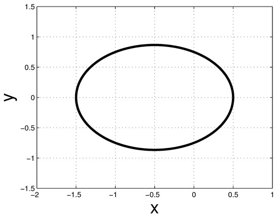
Figure 1. The reference solution for Kepler’s problem computed by integrating Equation (90) until the time $T=7$ using Verner’s method with the time step $h=2\times {10}^{-7}$.

We solved the same problem using several of the methods discussed in Section 4 for a number of time steps ranging from $h=3.5\times {10}^{-3}$ to $h=3.5\times {10}^{-1}$. The value of the solutions at $T=7$ was then compared against the reference solution. The max norm errors are depicted in Figure 2. We see that the rates of convergence of the Gauss and the 3-stage Radau IIA methods are consistent with Theorem 4 and Corollary 3. For the Lobatto IIIA-IIIB methods, we observe a reduction of order. The 2-stage Lobatto IIIA-IIIB method turns out to be inconsistent and is not depicted in Figure 2. Both the 3- and 4-stage methods converge only quadratically, while their classical orders of convergence are 4 and 6, respectively.

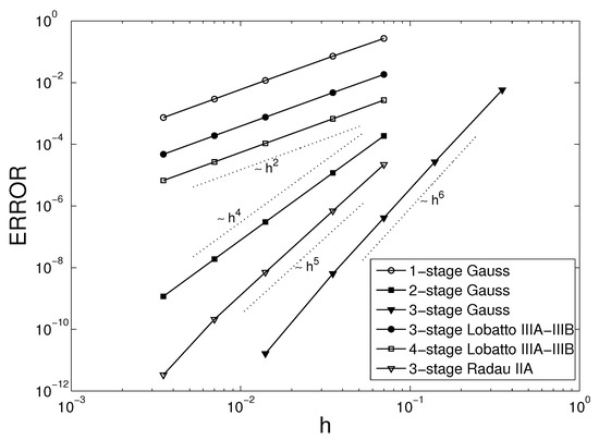
Figure 2. Convergence of several Runge–Kutta methods for Kepler’s problem.

We also investigated the long-time behavior of our integrators and conservation of the Hamiltonian. For convenience, we set $H_0=-0.5$ in Equation (112), so that $H=0$ on the considered orbit. We applied the Gauss methods with the relatively large time step $h=0.1$ and computed the numerical solution until the time $T=5\times {10}^5$. Figure 3 shows that the Gauss integrators preserve the Hamiltonian very well, which is consistent with Corollary 4. We performed similar computations for the Lobatto IIIA-IIIB and Radau IIA methods, also with $h=0.1$. The results are depicted in Figure 4. The 3- and 4-stage Lobatto IIIA-IIIB schemes result in instabilities, the planet’s trajectory spirals down on the center of gravity, and the computations cannot be continued too far in time. The Hamiltonian shows major variations whose amplitude grows in time. The non-variational Radau IIA scheme yields an accurate solution, but it demonstrates a gradual energy dissipation.

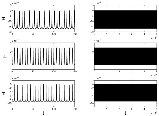
Figure 3. Hamiltonian conservation for the 1-stage (top row), 2-stage (middle row) and 3-stage (bottom row) Gauss methods applied to Kepler’s problem with the time step $h=0.1$ over the time interval $[0,5\times {10}^5]$ (right column), with a close-up on the initial interval $[0,150]$ shown in (left column).

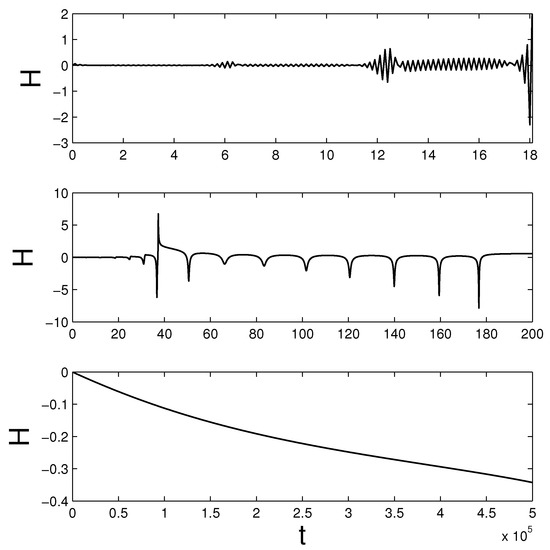
Figure 4. Hamiltonian for the numerical solution of Kepler’s problem obtained with the 3- and 4-stage Lobatto IIIA-IIIB schemes (top,middle), respectively, and the non-variational Radau IIA method (bottom).

5.2. Point Vortices

Point vortices in the plane are another interesting example of a system with linear ${\alpha }_{\mu }(q)$ (see [17,18,27]). A system of K interacting point vortices in two dimensions can be described by the Lagrangian

$$L(x_1,y_1,\dots ,x_K,y_K,{\dot{x}}_1,{\dot{y}}_1,\dots ,{\dot{x}}_K,{\dot{y}}_K)=\frac{1}{2}\sum _{i=1}^K{\mathsf{\Gamma }}_i(x_i{\dot{y}}_i-y_i{\dot{x}}_i)-H(x_1,y_1,\dots ,x_K,y_K)$$

(115)

with the Hamiltonian

$$H(x_1,y_1,\dots ,x_K,y_K)=\frac{1}{4\pi }\sum _{i<j}^K{\mathsf{\Gamma }}_i{\mathsf{\Gamma }}_{j}log\left({(x_i-x_j)}^2+{(y_i-y_j)}^2\right)-H_0,$$

(116)

where $(x_i,y_i)$ denotes the location of the i-th vortex, ${\mathsf{\Gamma }}_i$ is its circulation, and $H_0$ is an arbitrary constant.

As a test problem, we considered the system of $K=2$ vortices with circulations ${\mathsf{\Gamma }}_1=4$ and ${\mathsf{\Gamma }}_2=2$, respectively, and distance $D=1$ between them. The vortices rotate on concentric circles about their center of vorticity at $x_C=0$ and $y_C=0$. We took the initial condition at $x_1^{(0)}={\mathsf{\Gamma }}_{2}D/({\mathsf{\Gamma }}_1+{\mathsf{\Gamma }}_2)\approx 0.33$, $y_1^{(0)}=0$, $x_2^{(0)}=-{\mathsf{\Gamma }}_{1}D/({\mathsf{\Gamma }}_1+{\mathsf{\Gamma }}_2)\approx -0.67$ and $y_2^{(0)}=0$. The analytic solution can be found (see [27]) as

$$\begin{array}{ccc}\hfill x_1(t)& =\frac{{\mathsf{\Gamma }}_2}{{\mathsf{\Gamma }}_1+{\mathsf{\Gamma }}_2}Dcos\omega t,\hfill & \hfill x_2(t)=-\frac{{\mathsf{\Gamma }}_1}{{\mathsf{\Gamma }}_1+{\mathsf{\Gamma }}_2}Dcos\omega t,\\ \hfill y_1(t)& =\frac{{\mathsf{\Gamma }}_2}{{\mathsf{\Gamma }}_1+{\mathsf{\Gamma }}_2}Dsin\omega t,\hfill & \hfill y_2(t)=-\frac{{\mathsf{\Gamma }}_1}{{\mathsf{\Gamma }}_1+{\mathsf{\Gamma }}_2}Dsin\omega t,\end{array}$$

(117)

where $\omega =({\mathsf{\Gamma }}_1+{\mathsf{\Gamma }}_2)/(2\pi D^2)$. This is a periodic solution with period $T_{period}\approx 6.58$ (see Figure 5).

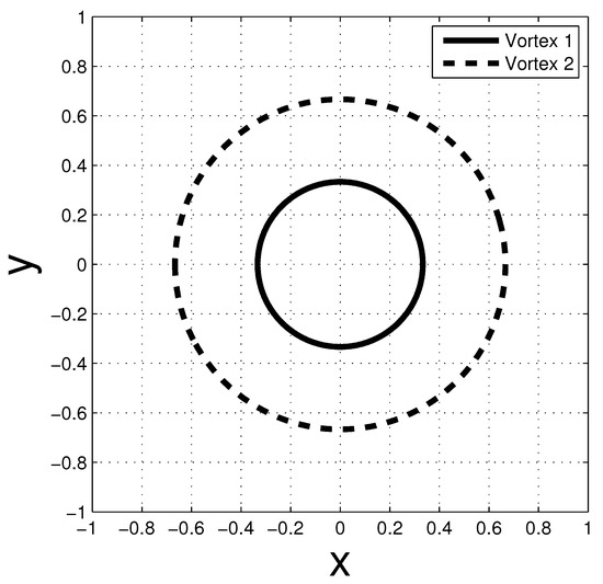
Figure 5. The circular trajectories of the two point vortices rotating about their vorticity center at $x_C=0$ and $y_C=0$.

We performed similar convergence tests as presented in Section 5.1. The value of the numerical solutions at time T = 7 were compared against the exact solution given in Equation (117). The max norm errors are depicted in Figure 6. The results are qualitatively the same as for Kepler’s problem.

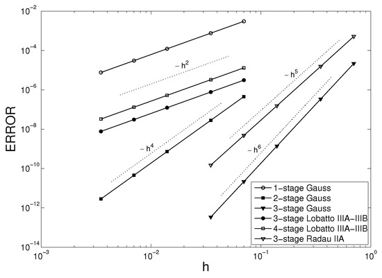
Figure 6. Convergence of several Runge–Kutta methods for the system of two point vortices.

We set $H_0=0$ in Equation (116), so that $H=0$ for the considered solution. Figure 7 and Figure 8 show the behavior of the numerical Hamiltonian over a long integration interval. The 3- and 4-stage Lobatto IIIA-IIIB integrators performed better than for Kepler’s problem. In the case of the Gauss methods, the Hamiltonian stayed virtually constant—the visible minor erratic oscillations are the result of round-off errors. The Radau IIA scheme demonstrated a slow but systematic drift.

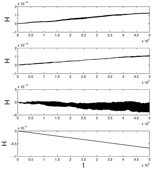
Figure 7. Hamiltonian for the 1-stage (top), 2-stage (second) and 3-stage (third) Gauss, and the 3-stage Radau IIA (bottom) methods applied to the system of two point vortices with the time step $h=0.1$ over the time interval $[0,5\times {10}^5]$.

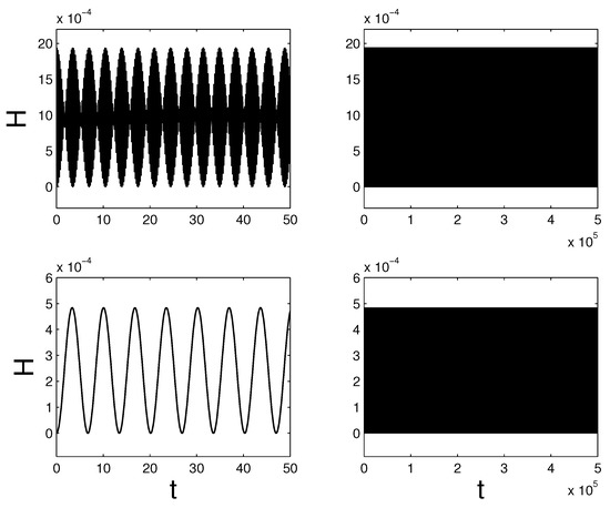
Figure 8. Hamiltonian conservation for the 3-stage (top) and 4-stage (bottom) Lobatto IIIA-IIIB methods applied to the system of two point vortices with the time step $h=0.1$ over the time interval $[0,5\times {10}^5]$ (right column), with a close-up on the initial interval $[0,50]$ shown in (left column).

5.3. Lotka–Volterra Model

The dynamics of the growth of two interacting (predator/prey) species can be modeled by the Lotka–Volterra equations

$$\begin{array}{cc}\hfill \dot{u}& =u(v-2),\hfill \\ \hfill \dot{v}& =v(1-u),\hfill \end{array}$$

(118)

where $u(t)$ denotes the number of predators and $v(t)$ the number of prey, and constants 1 and 2 were chosen arbitrarily. These equations can be rewritten as the Poisson system

$$\left(\begin{array}{c}\dot{u}\\ \dot{v}\end{array}\right)=\left(\begin{array}{cc}0& uv\\ -uv& 0\end{array}\right)DH(u,v),$$

(119)

where the Hamiltonian is given by

$$H(u,v)=u-logu+v-2logv-H_0$$

(120)

with an arbitrary constant $H_0$ (see [1]). Using an approach similar to the one presented in Section 5.1, one can easily verify that the Lagrangian

$$L(q,\dot{q})=\left(\frac{log{q}^2}{q^1}+q^2\right){\dot{q}}^1+q^1{\dot{q}}^2-H(q)$$

(121)

reproduces the same equations of motion, where $q=(u,v)$. The coordinates ${\alpha }_{\mu }(q)$ (cf. Equation (2)) were chosen, so that the assumptions of Theorem 2 are satisfied for the considered Runge–Kutta methods.

As a test problem, we considered the solution with the initial condition $q_{init}^1=1$ and $q_{init}^2=1$ (note that $q=(1,2)$ is an equilibrium point). This is a periodic solution with period $T_{period}\approx 4.66$. A reference solution was computed by integrating Equation (90) until the time $T=5$ using Verner’s method with the small time step $h={10}^{-7}$. The reference solution is depicted in Figure 9.

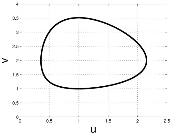
Figure 9. The reference solution for the Lotka–Volterra equations computed by integrating Equation (90) until the time $T=5$ using Verner’s method with the time step $h={10}^{-7}$.

Convergence plots are shown in Figure 10. The convergence rates for the Gauss and Radau IIA methods are consistent with the theoretical results presented in Section 4.3.1—we see that the orders of the 2- and 3-stage Gauss schemes are reduced. The 2-stage Lobatto IIIA-IIIB scheme again proves to be inconsistent, and the 3- and 4-stage schemes converge quadratically, just as in Section 5.1 and Section 5.2.

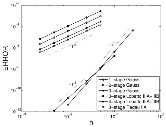
Figure 10. Convergence of several Runge–Kutta methods for the Lotka–Volterra model.

We performed another series of numerical experiments with the time step $h=0.1$ to investigate the long time behavior of the considered integrators. The results are shown in Figure 11 and Figure 12. We set $H_0=2$ in Equation (120), so that $H=0$ for the considered solution. The 1- and 3-stage Gauss methods again show excellent Hamiltonian conservation over a long time interval. The 2-stage Gauss method, however, does not perform equally well—the Hamiltonian oscillates with an increasing amplitude over time, until the computations finally break down. The Lobatto IIIA-IIIB methods show similar problems as in Section 5.1. The non-variational Radau IIA method yields an accurate solution, but demonstrates a steady drift in the Hamiltonian.

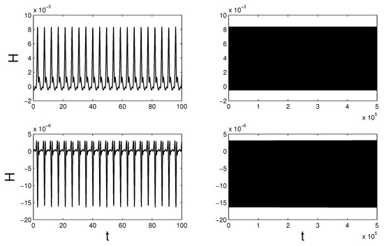
Figure 11. Hamiltonian conservation for the 1-stage (top row) and 3-stage (bottom row) Gauss methods applied to the Lotka–Volterra model with the time step $h=0.1$ over the time interval $[0,5\times {10}^5]$ (right column), with a close-up on the initial interval $[0,100]$ shown in (left column).

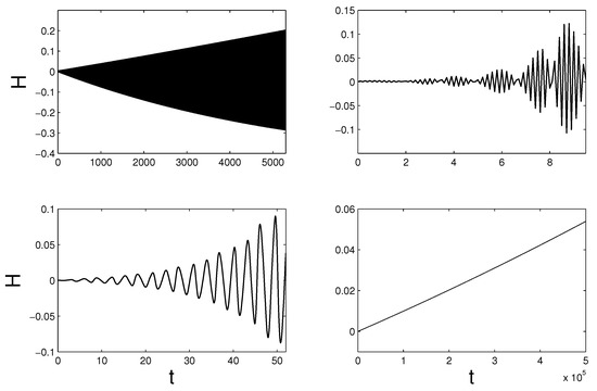
Figure 12. Hamiltonian for the numerical solution of the Lotka–Volterra model obtained with the 2-stage Gauss method (top left), the 3- and 4-stage Lobatto IIIA-IIIB schemes (top right,bottom left), respectively, and the non-variational Radau IIA method (bottom right).

6. Summary

We analyze a class of degenerate systems described by Lagrangians that are linear in velocities, and present a way to construct appropriate higher-order variational integrators. We point out how the theory underlying variational integration is different from the non-degenerate case and we made a connection with numerical integration of differential-algebraic equations. We also perform numerical experiments for several example models.

Our work can be extended in several ways. In Section 5.3, we present our numerical results for the Lotka–Volterra model, which is an example of a system for which the coordinate functions ${\alpha }_{\mu }(q)$ are nonlinear. The 1- and 3-stage Gauss methods perform exceptionally well and preserve the Hamiltonian over a very long integration time. It would be interesting to perform a backward error (or similar) analysis to check if this behavior is generic. If confirmed, our variational approach could provide a new way to construct geometric integrators for a broader class of Poisson systems. The study of modified Lagrangians recently presented in [48] is the first step towards a rigorous backward error analysis for the variational integrators considered in our work.

Another idea worth exploring is a construction of variational integrators that exactly satisfy the primary constraint. Certain advances in that direction were made in [49] by applying projection methods.

It would also be interesting to further consider constrained systems with Lagrangians that are linear in velocities and construct associated higher-order variational integrators. This would allow generalizing the space-adaptive methods presented in [24,50] to degenerate field theories, such as the nonlinear Schrödinger, KdV or Camassa–Holm equations.

References

- Hairer, E.; Lubich, C.; Wanner, G. Geometric Numerical Integration: Structure-Preserving Algorithms for Ordinary Differential Equations; Springer Series in Computational Mathematics; Springer: New York, NY, USA, 2002. [Google Scholar]
- McLachlan, R.I.; Quispel, G.R.W. Geometric integrators for ODEs. J. Phys. A Math. Gen. 2006, 39, 5251–5285. [Google Scholar] [CrossRef]
- Sanz-Serna, J.M. Symplectic integrators for Hamiltonian problems: an overview. Acta Numer. 1992, 1, 243–286. [Google Scholar] [CrossRef]
- Marsden, J.E.; West, M. Discrete mechanics and variational integrators. Acta Numer. 2001, 10, 357–514. [Google Scholar] [CrossRef]
- Bou-Rabee, N.; Owhadi, H. Stochastic variational integrators. IMA J. Numer. Anal. 2009, 29, 421–443. [Google Scholar] [CrossRef]
- Bou-Rabee, N.; Owhadi, H. Stochastic Variational Partitioned Runge-Kutta Integrators for Constrained Systems. arXiv 2007, arXiv:0709.2222. [Google Scholar]
- Kraus, M.; Tyranowski, T.M. Variational integrators for stochastic dissipative Hamiltonian systems. arXiv 2019, arXiv:1904.06205. [Google Scholar]
- Hall, J.; Leok, M. Spectral Variational Integrators. Numer. Math. 2015, 130, 681–740. [Google Scholar] [CrossRef]
- Holm, D.D.; Tyranowski, T.M. Variational principles for stochastic soliton dynamics. Proc. R. Soc. Lond. A Math. Phys. Eng. Sci. 2016, 472. [Google Scholar] [CrossRef]
- Holm, D.D.; Tyranowski, T.M. Stochastic discrete Hamiltonian variational integrators. BIT Numer. Math. 2018, 58, 1009–1048. [Google Scholar] [CrossRef]
- Jay, L.O. Structure Preservation for Constrained Dynamics with Super Partitioned Additive Runge–Kutta Methods. SIAM J. Sci. Comput. 1998, 20, 416–446. [Google Scholar]
- Kane, C.; Marsden, J.E.; Ortiz, M.; West, M. Variational integrators and the Newmark algorithm for conservative and dissipative mechanical systems. Int. J. Numer. Methods Eng. 2000, 49, 1295–1325. [Google Scholar] [CrossRef]
- Leok, M.; Shingel, T. General techniques for constructing variational integrators. Front. Math. China 2012, 7, 273–303. [Google Scholar] [CrossRef]
- Leok, M.; Zhang, J. Discrete Hamiltonian variational integrators. IMA J. Numer. Anal. 2011, 31, 1497–1532. [Google Scholar] [CrossRef]
- Ober-Blöbaum, S. Galerkin variational integrators and modified symplectic Runge-Kutta methods. IMA J. Numer. Anal. 2017, 37, 375–406. [Google Scholar] [CrossRef]
- Ober-Blöbaum, S.; Saake, N. Construction and analysis of higher order Galerkin variational integrators. Adv. Comput. Math. 2015, 41, 955–986. [Google Scholar] [CrossRef]
- Rowley, C.W.; Marsden, J.E. Variational integrators for degenerate Lagrangians, with application to point vortices. In Proceedings of the 41st IEEE Conference on Decision and Control, Las Vegas, NV, USA, 10–13 December 2002; Volume 2, pp. 1521–1527. [Google Scholar]
- Vankerschaver, J.; Leok, M. A novel formulation of point vortex dynamics on the sphere: Geometrical and numerical aspects. J. Nonlin. Sci. 2014, 24, 1–37. [Google Scholar] [CrossRef]
- Marsden, J.E.; Patrick, G.W.; Shkoller, S. Multisymplectic geometry, variational integrators, and nonlinear PDEs. Commun. Math. Phys. 1998, 199, 351–395. [Google Scholar] [CrossRef]
- Holm, D.D.; Tyranowski, T.M. New variational and multisymplectic formulations of the Euler–Poincaré equation on the Virasoro–Bott group using the inverse map. Proc. R. Soc. Lond. A Math. Phys. Eng. Sci. 2018, 474. [Google Scholar] [CrossRef] [PubMed]
- Lew, A.; Marsden, J.E.; Ortiz, M.; West, M. Asynchronous variational integrators. Arch. Ration. Mech. Anal. 2003, 167, 85–146. [Google Scholar] [CrossRef]
- Pavlov, D.; Mullen, P.; Tong, Y.; Kanso, E.; Marsden, J.E.; Desbrun, M. Structure-preserving discretization of incompressible fluids. Phys. D Nonlinear Phenom. 2011, 240, 443–458. [Google Scholar] [CrossRef]
- Stern, A.; Tong, Y.; Desbrun, M.; Marsden, J.E. Variational integrators for Maxwell’s equations with sources. PIERS Online 2008, 4, 711–715. [Google Scholar] [CrossRef]
- Tyranowski, T.M.; Desbrun, M. R-Adaptive Multisymplectic and Variational Integrators. Mathematics 2019, 7, 642. [Google Scholar] [CrossRef]
- Gotay, M. Presymplectic Manifolds, Geometric Constraint Theory and the Dirac-Bergmann Theory of Constraints. Ph.D. Thesis, University of Maryland, College Park, MD, USA, 1979. [Google Scholar]
- Marsden, J.; Ratiu, T. Introduction to Mechanics and Symmetry. Texts in Applied Mathematics; Springer: New York, NY, USA, 1994; Volume 17. [Google Scholar]
- Newton, P. The N-Vortex Problem: Analytical Techniques; Applied Mathematical Sciences; Springer: New York, NY, USA, 2001; Volume 145. [Google Scholar]
- Ellison, C.L.; Finn, J.M.; Qin, H.; Tang, W.M. Development of variational guiding center algorithms for parallel calculations in experimental magnetic equilibria. Plasma Phys. Control. Fusion 2015, 57, 054007. [Google Scholar] [CrossRef]
- Ellison, C.L. Development of Multistep and Degenerate Variational Integrators for Applications in Plasma Physics. Ph.D. Thesis, Princeton University, Princeton, NJ, USA, 2016. [Google Scholar]
- Ellison, C.L.; Finn, J.M.; Burby, J.W.; Kraus, M.; Qin, H.; Tang, W.M. Degenerate variational integrators for magnetic field line flow and guiding center trajectories. Phys. Plasmas 2018, 25, 052502. [Google Scholar] [CrossRef]
- Qin, H.; Guan, X. Variational Symplectic Integrator for Long-Time Simulations of the Guiding-Center Motion of Charged Particles in General Magnetic Fields. Phys. Rev. Lett. 2008, 100, 035006. [Google Scholar] [CrossRef] [PubMed]
- Qin, H.; Guan, X.; Tang, W.M. Variational symplectic algorithm for guiding center dynamics and its application in tokamak geometry. Phys. Plasmas 2009, 16, 042510. [Google Scholar] [CrossRef]
- Faou, E. Geometric Numerical Integration and Schrödinger Equations; Zurich Lectures in Advanced Mathematics; European Mathematical Society: Zürich, Switzerland, 2012. [Google Scholar]
- Drazin, P.; Johnson, R. Solitons: An Introduction; Cambridge Computer Science Texts; Cambridge University Press: Cambridge, UK, 1989. [Google Scholar]
- Gotay, M. A multisymplectic approach to the KdV equation. In Differential Geometric Methods in Theoretical Physics; NATO Advanced Science Institutes Series C: Mathematical and Physical Sciences; Springer: Dordrecht, The Netherlands, 1988; Volume 250, pp. 295–305. [Google Scholar]
- Camassa, R.; Holm, D.D. An integrable shallow water equation with peaked solitons. Phys. Rev. Lett. 1993, 71, 1661–1664. [Google Scholar] [CrossRef] [PubMed]
- Camassa, R.; Holm, D.D.; Hyman, J. A new integrable shallow water equation. Adv. App. Mech. 1994, 31, 1–31. [Google Scholar]
- Ergenç, T.; Karasözen, B. Poisson integrators for Volterra lattice equations. Appl. Numer. Math. 2006, 56, 879–887. [Google Scholar] [CrossRef][Green Version]
- Karasözen, B. Poisson integrators. Math. Comput. Model. 2004, 40, 1225–1244. [Google Scholar] [CrossRef]
- Suris, Y.B. Integrable discretizations for lattice system: local equations of motion and their Hamiltonian properties. Rev. Math. Phys. 1999, 11, 727–822. [Google Scholar] [CrossRef]
- Hairer, E.; Wanner, G. Solving Ordinary Differential Equations II: Stiff and Differential-Algebraic Problems, 2nd ed.; Springer Series in Computational Mathematics; Springer: Berlin, Gremany, 1996; Volume 14. [Google Scholar]
- Lubich, C. Integration of stiff mechanical systems by Runge-Kutta methods. Zeitschrift für Angewandte Mathematik und Physik ZAMP 1993, 44, 1022–1053. [Google Scholar] [CrossRef][Green Version]
- Rabier, P.J.; Rheinboldt, W.C. Theoretical and Numerical Analysis of Differential-Algebraic Equations. In Handbook of Numerical Analysis; Ciarlet, P.G., Lion, J.L., Eds.; Elsevier Science B.V.: Amsterdam, The Netherlands, 2002; Volume 8, pp. 183–540. [Google Scholar]
- Hairer, E.; Nørsett, S.; Wanner, G. Solving Ordinary Differential Equations I: Nonstiff Problems, 2nd ed.; Springer Series in Computational Mathematics; Springer: Berlin, Germany, 1993; Volume 8. [Google Scholar]
- Hairer, E.; Lubich, C.; Roche, M. The Numerical Solution of Differential-algebraic Systems by Runge-Kutta Methods; Lecture Notes in Math. 1409; Springer: Berlin, Germany, 1989. [Google Scholar]
- Brenan, K.; Campbell, S.; Petzold, L. Numerical Solution of Initial-Value Problems in Differential-Algebraic Equations; Classics in Applied Mathematics; Society for Industrial and Applied Mathematics: Philadelphia, PA, USA, 1996. [Google Scholar]
- Faddeev, L.; Jackiw, R. Hamiltonian reduction of unconstrained and constrained systems. Phys. Rev. Lett. 1988, 60, 1692–1694. [Google Scholar] [CrossRef] [PubMed]
- Vermeeren, M. Modified equations for variational integrators applied to Lagrangians linear in velocities. J. Geom. Mech. 2019, 11, 1–22. [Google Scholar] [CrossRef]
- Kraus, M. Projected Variational Integrators for Degenerate Lagrangian Systems. arXiv 2017, arXiv:1708.07356. [Google Scholar]
- Tyranowski, T.M. Geometric Integration Applied to Moving Mesh Methods and Degenerate Lagrangians. Ph.D. Thesis, California Institute of Technology, Pasadena, CA, USA, 2014. [Google Scholar]
© 2019 by the authors. Licensee MDPI, Basel, Switzerland. This article is an open access article distributed under the terms and conditions of the Creative Commons Attribution (CC BY) license (http://creativecommons.org/licenses/by/4.0/).