Exponential Stability Results on Random and Fixed Time Impulsive Differential Systems with Infinite Delay

Abstract

In this paper, we investigated the stability criteria like an exponential and weakly exponential stable for random impulsive infinite delay differential systems (RIIDDS). Furthermore, we proved some extended exponential and weakly exponential stability results for RIIDDS by using the Lyapunov function and Razumikhin technique. Unlike other studies, we show that the stability behavior of the random time impulses is faster than the fixed time impulses. Finally, two examples were studied for comparative results of fixed and random time impulses it shows by simulation.

1. Introduction

Impulses occur in a short duration of time which makes a sudden change in the nature or behavior of the differential system; we call this system an impulsive differential system. Most of the impulsive differential equation models deal with the fixed time of occurrence of impulse action. Many authors contributed to analyzing the fixed time impulsive differential systems (IDS) with the finite or infinite delay because this system arises in many fields like science, engineering, biotechnology, neural networks, and control systems—see the monographs [1,2]. The study of qualitative behavior like the stability of impulsive differential systems is also important. Generally, stability behavior for IDS with delays can have two types of results: (i) impulsive perturbation and (ii) impulsive stabilization. For the past several decades, many authors have studied the stability behavior of various types of impulsive systems by using the Lyapunov functions and Razumikhin technique. Moreover, the Lyapunov functional method plays an important role in the stability theory of functional differential systems it used to obtain the minimal class of functional from the corresponding derivative of the Lyapunov functions; for example, in [3,4], the authors proved the exponential stability by using the Lyapunov and Razumikhin technique and the authors in [5,6,7] investigated the Razumikhin-type theorems for weakly exponentially stable and exponentially stable. Recently, the authors in [8] established some new Razumikhin-technique for studying the uniform stability behavior of the systems. However, impulses used to control for the unstable differential systems can be stabilized to the equilibrium point; this is shown in [9,10]. Furthermore, several interesting results have been established in [11,12,13,14,15,16] and the references therein. However, the impulses happen not only in fixed time on the system states, but it is also possible to happen randomly; we know that the real world system states often change randomly. From this point of view, we develop random impulses in differential systems.

Very few attempts are made in the study of the random time occurrence of impulses. This changing nature from a deterministic system to a stochastic system differs from the stochastic differential equation—for example, in [17], the authors investigated the existence, uniqueness and stability results for random IDS. In [18], the author studied the $p^{th}$ moment exponential stability results and the authors [19] discussed the distribution nature for random IDS and proved the exponential stability. For further study, refer to [20,21,22,23,24,25,26,27,28,29] and references therein. Still, now there was no paper reported on the exponential stability for RIIDDS based on the Lyapunov and Razumikhin approach. Therefore, it is necessary to identify the exponential stability results for RIIDDS.

Inspired by the above discussions in this paper, we construct some new sufficient conditions for exponential stability by employing the random impulses. Furthermore, we discuss the random time impulses are faster than fixed time impulses. Finally, we show the stability behavior of random time impulses and the fixed time impulses. The rest of this paper is as follows: there are some definitions and lemmas in the preliminaries in Section 2. In Section 3, we prove the exponential stability and weakly exponential stability results for RIIDDS by using the Lyapunov and Razumikhin technique. Then, in Section 4, two numerical examples and their simulations are discussed and, finally, in Section 5, conclusions are given.

Notations: Let ℜ denote the set of all real numbers, ${\Re }_{+}$ the set of all non-negative real numbers and $Z_{+}$ the set of all positive integers. Let ${\Re }^n$ be the Euclidean space equipped with norm $∥·∥$, and $(\mathsf{\Omega },\mathcal{F},P)$ be a probability space. We use $\mathsf{\Gamma }=\mathcal{PC}\left(\left(-\infty ,0\right],{\Re }^n\right)$ to denote the set of all piecewise right continuous real valued random variables $\phi :(-\infty ,0]\to {\Re }^n$ with the norm is defined by ${\displaystyle {E\parallel \phi \parallel }^p=\underset{\theta \in (-\infty ,0]}{sup}E{\parallel \phi \left(\theta \right)\parallel }^p}$. The symbol $PC\mathcal{B}\left(t\right)$ denotes a set of all bounded piecewise right continuous real valued random variables $\phi$. Then, $E(·)$ stands for the expectation operator with respect to the given P. Moreover, letting $\widehat{\mathcal{C}}=C({\Re }_{+},{\Re }_{+})$, we define: $K_1=\{\nu \in \widehat{\mathcal{C}}|\nu \left(0\right)=0$$\mathrm{and}\nu \left(s\right)>0\mathrm{for}s>0\}$; $K_2=\{\nu \in \widehat{\mathcal{C}}|\nu \left(0\right)=0\mathrm{and}\nu \left(s\right)>0\mathrm{for}s>0\mathrm{and}\nu \mathrm{is}\mathrm{nondecreasing}\mathrm{in}\mathrm{s}\}$; $K_3=\{\nu \in \widehat{\mathcal{C}}|\nu \left(0\right)=0$$\mathrm{and}\nu \left(s\right)>0\mathrm{for}s>0\mathrm{and}\nu \mathrm{is}\mathrm{strictly}\mathrm{increasing}\mathrm{in}\mathrm{s}\}$.

2. Preliminaries

Let ${\left\{{\tau }_m^{{}^{\prime }}\right\}}_{m=1}^{\infty }$ be a sequence of independent exponentially distributed random variables with parameter $\gamma$ defined on sample space $\mathsf{\Omega }$ and ${\left\{{\xi }_m^{{}^{\prime }}\right\}}_{m=0}^{\infty }$ be the increasing sequence of random variables. Note that ${\xi }_0^{{}^{\prime }}=t_0$, where $t_0\ge 0$ is a fixed point and ${\xi }_m^{{}^{\prime }}={\xi }_{m-1}^{{}^{\prime }}+{\tau }_m^{{}^{\prime }}$ for $m=1,2,\cdots$, where ${\tau }_m^{{}^{\prime }}$ defines the waiting time between two consecutive impulses and provides ${\displaystyle \sum _{m=1}^{\infty }}{\tau }_m^{{}^{\prime }}=\infty$ with probability 1.

Let us consider the delay differential systems with random impulses of the form

$$\begin{array}{ccc}\hfill y^{\prime }\left(t\right)& =& g(t,y_t),{\xi }_m^{{}^{\prime }}<t<{\xi }_{m+1}^{{}^{\prime }},t\ge t_0,\hfill \\ \hfill y\left({\xi }_m^{{}^{\prime }+}\right)& =& I_m({\xi }_m^{{}^{\prime }},y\left({\xi }_m^{{}^{\prime }-}\right)),m=1,2,\cdots ,\hfill \\ \hfill y\left(\theta \right)& =& \varphi \left(\theta \right),\theta \in (-\infty ,0],\hfill \end{array}$$

(1)

where $\varphi \in \mathsf{\Gamma }$ and $g\in C([0,\infty )\times D,{\Re }^n)$, $g(t,0)=0$, where D is an open set in $\mathsf{\Gamma }$. For any $t\ge t_0,y_t=\{y(t+\theta ),\theta \in (-\infty ,0]\}$. For any $m=1,2,3,\cdots ,I_m(t,y)\in C([0,\infty )\times {\Re }^n,{\Re }^n),I_m({\xi }_m^{{}^{\prime }},0)=0$ and for any $\rho >0$, there exists ${\rho }_1>0({\rho }_1<\rho )$ such that $y\in S\left({\rho }_1\right)$ implies that $y+I_m({\xi }_m^{{}^{\prime }},y)\in S\left(\rho \right)$, where $S\left(\rho \right)=\left\{y:∥y∥<\rho ,y\in {\Re }^n\right\}$. For any $t_0\ge 0$, let $PC{\mathcal{B}}_{\delta }\left(t_0\right)=\left\{\phi \in PC\mathcal{B}\left(t_0\right):∥\phi ∥<\delta \right\}$, and let $\phi \left(\theta \right)=y(t+\theta )$, thus $\phi \left(0\right)=y\left(t\right)$. Furthermore, we define $y\left({\xi }_m^{{}^{\prime }+}\right)$ and $y\left({\xi }_m^{{}^{\prime }-}\right)$ are the right and left limits at ${\xi }_m^{{}^{\prime }}$.

We assume the existence and uniqueness solution for the initial value problem (1), and denoted as $y(t,t_0,\varphi )$. Since $g(t,0)=0,I_m({\xi }_m^{{}^{\prime }},0)=0,m=1,2,\dots$, then $y\left(t\right)=0$ is the trivial solution of system (1).

Remark 1.

Define ${\left\{{\xi }_m\right\}}_{m=0}^{\infty }$ be the increasing sequence of points, where ${\xi }_m$ is a value of the corresponding random variable ${\xi }_m^{{}^{\prime }},\forall m=1,2,\cdots$, and ${\left\{{\tau }_m\right\}}_{m=1}^{\infty }$ is a sequence of points, where ${\tau }_m$ are arbitrary values of the random variable ${\tau }_m^{{}^{\prime }},\forall m=1,2,\cdots$. For convenience, we define ${\xi }_0=t_0$ and ${\xi }_m={\xi }_{m-1}+{\tau }_m,\forall m=1,2,\cdots$, where ${\tau }_m$ denotes the value of the waiting time. Then, system (1) becomes

$$\begin{array}{ccc}\hfill y^{\prime }\left(t\right)& =& g(t,y_t),t\ne {\xi }_m,t\ge t_0,\hfill \\ \hfill y\left({\xi }_m^{+}\right)& =& I_m({\xi }_m,y\left({\xi }_m^{-}\right)),m=1,2,\cdots ,\hfill \\ \hfill y\left(\theta \right)& =& \varphi \left(\theta \right),\theta \in (-\infty ,0].\hfill \end{array}$$

(2)

The solution of system (2) depends not only on the initial condition; it also depends on the moments of impulses ${\xi }_m,m=1,2,\cdots$. That is, the solution depends on the chosen arbitrary values ${\tau }_m$ of the random variable ${\tau }_m^{{}^{\prime }},\forall m=1,2,\cdots$. We denote the solution of (2) by $y(t;t_0,\varphi ,\left\{{\tau }_m\right\})$ and will assume $y\left({\xi }_m\right)=\underset{t\to {\xi }_m-0}{lim}y\left(t\right)$.

Moreover, the collection of all solutions of system (2) is called a sample path solution of system (1). Thus, the sample path solution generates a stochastic process. We will say that it is a solution of system (1), and it is denoted by $y(t;t_0,\varphi ,\left\{{\tau }_m^{{}^{\prime }}\right\})$.

Lemma 1.

From [19,28], when there will be exactly m impulses until the time $t,t\ge t_0$, and the waiting time between two consecutive impulses follow exponential distribution with parameter γ, then the probability

$$P\left(I_{[{\xi }_m^{{}^{\prime }},{\xi }_{m+1}^{{}^{\prime }})}\left(t\right)\right)=\frac{{\gamma }^m{(t-t_0)}^m}{m!}{e}^{-\gamma (t-t_0)},$$

where the events $I_{[{\xi }_m^{{}^{\prime }},{\xi }_{m+1}^{{}^{\prime }})}\left(t\right)=\{\omega \in \mathsf{\Omega }:{\xi }_m^{{}^{\prime }}\left(\omega \right)<t<{\xi }_{m+1}^{{}^{\prime }}\left(\omega \right)\},m=1,2,\cdots$.

Remark 2.

From [19,28], if $y\left(t\right)$ is the solution of the random impulsive differential equations, then

$$E[\parallel y\left(t\right)\parallel ]=\sum _{m=0}^{\infty }E[\parallel y\left(t\right)\parallel |I_{[{\xi }_m^{{}^{\prime }},{\xi }_{m+1}^{{}^{\prime }})}\left(t\right)]P\left(I_{[{\xi }_m^{{}^{\prime }},{\xi }_{m+1}^{{}^{\prime }})}\left(t\right)\right),$$

where ${\xi }_m^{{}^{\prime }}$ is the impulse moments.

Definition 1.

The function $W:\Re \times \mathsf{\Gamma }⟶{\Re }_{+}$ belongs to class ${\omega }_0$ if

(i) 

W is continuous differentiable almost every where function.

(ii) 

$W(t,y)$ is locally Lipschitzian with respect to y and $W(t,0)\equiv 0$.

Definition 2.

Letting $W\in {\omega }_0$, for any $(t,\phi )\in [0,\infty )\times D$, the upper right hand Dini derivative of $W(t,y)$ along the solution of system (1) is defined by

$$\begin{array}{c}\hfill D^{+}W(t,\phi \left(0\right))=\underset{h\to 0^{+}}{lim\; sup}\left\{\frac{\left[W(t+h,\phi (0)+hg(t,\phi \left)\right)-W(t,\phi (0\left)\right)\right]}{h}\right\}.\end{array}$$

Definition 3.

Let $y\left(t\right)$ be a the solution of (1) through $(t_0,\varphi )$, and $p>0$. Then, the trivial solution of (1) is said to be

(i) 

$p^{th}$ moment weakly exponentially stable, assume $\alpha \left(s\right)\in K_3,\lambda >0$ is a constant (convergence rate), if for any $ϵ>0$, there exists $\delta =\delta \left(ϵ\right)>0$ such that $\varphi \in PC{\mathcal{B}}_{\delta }\left(t_0\right)$ implies $E\left[{\alpha }_1\left({∥y\left(t\right)∥}^p\right)\right]<ϵ·e^{-\lambda (t-t_0)},t\ge t_0$.

(ii) 

$p^{th}$ moment exponentially stable, assume $\lambda >0$ is a constant (convergence rate), if for any $ϵ>0$, there exists $\delta =\delta \left(ϵ\right)>0$ such that $\varphi \in PC{\mathcal{B}}_{\delta }\left(t_0\right)$ implies $E\left({∥y\left(t\right)∥}^p\right)<ϵ·e^{-\lambda (t-t_0)},t\ge t_0$.

3. Main Results

Theorem 1.

Assume that there exist functions ${\beta }_1,{\beta }_2\in K_1,h\in K_2,c\in \widehat{\mathcal{C}}$ and $q\in PC({\Re }_{+},{\Re }_{+}),W(t,y)\in {\omega }_0,$ and constants $\mathcal{M}>1,\lambda >0,w_m>0,\kappa >0$, such that $E\left[w_m\right]\le \kappa ,m\in Z_{+}$, and the following conditions hold:

(i) 

${\beta }_1\left({∥y∥}^p\right)\le W(t,y)\le {\beta }_2\left({∥y∥}^p\right),(t,y)\in \Re \times S\left(\rho \right);$

(ii) 

For any $\phi \in PC\left(\right(-\infty ,0],S(\rho \left)\right)$, if $h\left(W(t,\phi \left(0\right))e^{\lambda (t-t_0)}\right)\ge {\mathcal{M}}^{-1}W(t+\theta ,\phi \left(\theta \right)),\theta \in (-\infty ,0],$${\xi }_m^{{}^{\prime }}<t<{\xi }_{m+1}^{{}^{\prime }}$, then $D^{+}W(t,\phi \left(0\right))\le -q\left(t\right)c\left(W(t,\phi \left(0\right))\right)$, where $s<h\left(s\right)\le \mathcal{M}s$ for any $s>0$;

(iii) 

For all $({\xi }_m^{{}^{\prime }},\phi )\in {\Re }_{+}\times PC((-\infty ,0],S\left({\rho }_1\right)),W({\xi }_m^{{}^{\prime }},\phi \left(0\right)+I_m({\xi }_m^{{}^{\prime }},\phi ))\le w_{m}W({\xi }_m^{{}^{\prime }-},\phi \left(0\right))$, with $\left\{{\displaystyle \prod _{i=1}^{\infty }}E\left[w_i\right]\right\}\le \mathcal{M}$,

(iv) 

${\tau }^{{}^{\prime }}=\underset{m\in Z_{+}}{max}\left\{{\xi }_m^{{}^{\prime }}-{\xi }_{m-1}^{{}^{\prime }}\right\}<\infty ,{\mu }^{{}^{\prime }}=\underset{m\in Z_{+}}{min}\left\{{\xi }_m^{{}^{\prime }}-{\xi }_{m-1}^{{}^{\prime }}\right\}>0,\underset{t\ge 0}{inf}{\int }_t^{t+{\mu }^{{}^{\prime }}}q\left(s\right)ds=M_1<\infty ,\underset{s>0}{sup}{\int }_s^{s\mathcal{M}{e}^{\lambda {\tau }^{{}^{\prime }}}}\frac{dt}{c\left(t\right)}=M_2<M_1;$

(v) 

The inequality $\underset{s>0}{inf}q\left(s\right)·\underset{s>0}{inf}\frac{c\left(s\right)}{s}\ge \lambda$ holds.

Then, (1) is $p^{th}$ moment weakly exponentially stable.

Proof. 

Condition $\left(i\right)⟹{\beta }_1\left(s\right)\le {\beta }_2\left(s\right)$ for $s\in [0,\rho ]$.

Let ${\alpha }_1$ and ${\alpha }_2$ be strictly non-decreasing continuous functions satisfying ${\alpha }_1\left(s\right)\le {\beta }_1\left(s\right)\le {\beta }_2\left(s\right)\le {\alpha }_2\left(s\right)$, $\forall s\in [0,\rho ]$. Thus, we have

$$\begin{array}{c}\hfill {\alpha }_1\left({∥y∥}^p\right)\le W(t,y)\le {\alpha }_2\left({∥y∥}^p\right),\forall (t,y)\in \Re \times S\left(\rho \right).\end{array}$$

For any ${\rho }_1>0$ and $ϵ>0$, we may choose $\delta =\delta \left(ϵ\right)>0$, such that ${\alpha }_2\left(\delta \right)\le {\mathcal{M}}^{-2}min\left\{{\alpha }_1\left(ϵ\right),ϵ\right\}$.

Let $y\left(t\right),t\ge t_0$ be a solution of system (1) through $(t_0,\varphi )$, and it follows a stochastic process. For any $\varphi \in PC{\mathcal{B}}_{\delta }\left(t_0\right)$, we shall prove that

$$\begin{array}{c}\hfill E\left[{\alpha }_1\left({∥y\left(t\right)∥}^p\right)\right]\le ϵ·e^{-[\lambda +\gamma (1-\kappa )](t-t_0)},t\ge t_0.\end{array}$$

(3)

We will prove (3) with the aid of the sample path solution of (1). Thus, first, it is enough to prove that there are m impulses moments until time $t,t\ge t_0$,

$$\begin{array}{ccc}\hfill {\alpha }_1\left({∥y\left(t\right)∥}^p\right)& \le & ϵ·\prod _{i=1}^m{w}_i{e}^{-\lambda (t-t_0)},t\in [{\xi }_m,{\xi }_{m+1}),m=0,1,2,\cdots .\hfill \end{array}$$

For convenience, let $W\left(t\right)=W(t,y(t\left)\right)$, and $V\left(t_0\right)=max\left\{\underset{\theta \in (-\infty ,0]}{sup}W(t_0+\theta ,\phi \left(\theta \right)),\mathcal{M}W\left(t_0\right)\right\}$, which implies

$$\begin{array}{c}\hfill V\left(t_0\right)\le {\alpha }_2\left(\delta \right)\mathcal{M},\mathrm{in}\mathrm{view}\mathrm{of}(\phi \in PC{\mathcal{B}}_{\delta }\left(t_0\right)).\end{array}$$

We shall prove that there are $m=k$ impulses moments until time $t,t\ge t_0$,

$$\begin{array}{c}\hfill W\left(t\right)\le V\left(t_0\right)\prod _{i=1}^k{w}_i{e}^{-\lambda (t-t_0)},t\in [{\xi }_k,{\xi }_{k+1}).\end{array}$$

(4)

First, it is clear that, for $t\in (-\infty ,t_0)$,

$$\begin{array}{ccc}\hfill {\alpha }_1\left({∥y\left(t\right)∥}^p\right)& \le & W\left(t\right)\le V\left(t_0\right)\hfill \\ & <& \mathcal{M}{\alpha }_2\left(\delta \right)\hfill \\ & \le & {\mathcal{M}}^{-1}min\left\{{\alpha }_1\left(ϵ\right),ϵ\right\}\hfill \\ & \le & {\alpha }_1\left(ϵ\right).\hfill \end{array}$$

(5)

Thus, ${∥y\left(t\right)∥}^p<ϵ<{\rho }_1,t\in (-\infty ,t_0]$. Assuming $k=0$, i.e., no impulse moments, then we prove that

$$\begin{array}{c}\hfill W\left(t\right)e^{\lambda (t-t_0)}\le V\left(t_0\right),t\in [t_0,{\xi }_1).\end{array}$$

(6)

Supposing not, then there exists $t\in [t_0,{\xi }_1)$ such that $W\left(t\right)e^{\lambda (t-t_0)}>V\left(t_0\right)$. Let

$$\begin{array}{c}\hfill \widehat{t}=inf\left\{t\in [t_0,{\xi }_1)|W\left(t\right)e^{\lambda (t-t_0)}\ge V\left(t_0\right)\right\}.\end{array}$$

Then, $\widehat{t}\in (t_0,{\xi }_1)$, $W\left(\widehat{t}\right)e^{\lambda (\widehat{t}-t_0)}=V\left(t_0\right)$. In addition, $W\left(t\right)e^{\lambda (t-t_0)}<V\left(t_0\right),t\in [t_0,\widehat{t})$. Since

$$\begin{array}{c}\hfill W\left(t\right)e^{\lambda (t-t_0)}<V\left(t_0\right),\forall t\in (-\infty ,\widehat{t}).\end{array}$$

(7)

Note $h\left(W\left(\widehat{t}\right)e^{\lambda (\widehat{t}-t_0)}\right)=h\left(V\left(t_0\right)\right)>V\left(t_0\right)$, and $h\left(W\left(t_0\right)\right)\le h\left({\mathcal{M}}^{-1}V\left(t_0\right)\right)\le V\left(t_0\right)$, in view of $h\left(s\right)\le \mathcal{M}s$, thus define

$$\begin{array}{c}\hfill t^{*}=sup\left\{t\in [t_0,\widehat{t}]|h\left(W\left(t\right)e^{\lambda (t-t_0)}\right)\le V\left(t_0\right)\right\}.\end{array}$$

Thus, $t^{*}\in [t_0,\widehat{t}),h\left(W\left(t^{*}\right)e^{\lambda (t^{*}-t_0)}\right)=V\left(t_0\right)$, and $h\left(W\left(t\right)e^{\lambda (t-t_0)}\right)>V\left(t_0\right),t\in (t^{*},\widehat{t}]$. Hence, for $t\in [t^{*},\widehat{t}],s\in (-\infty ,t]$, considering (7), we have

$$\begin{array}{c}\hfill h\left(W\left(t\right)e^{\lambda (t-t_0)}\right)\ge V\left(t_0\right)\ge W\left(s\right)>{\mathcal{M}}^{-1}W\left(s\right).\end{array}$$

By $\left(ii\right)$, $D^{+}W\left(t\right)\le -q\left(t\right)c\left(W\left(t\right)\right)$ holds for all $t\in [t^{*},\widehat{t}]$. Therefore, we obtain

$$\begin{array}{ccc}\hfill D^{+}\left(W\left(t\right)e^{\lambda (t-t_0)}\right)& =& D^{+}W\left(t\right)e^{\lambda (t-t_0)}+\lambda W\left(t\right)e^{\lambda (t-t_0)}\hfill \\ & =& e^{\lambda (t-t_0)}(D^{+}W\left(t\right)+\lambda W\left(t\right))\hfill \\ & \le & e^{\lambda (t-t_0)}(-q\left(t\right)c\left(W\left(t\right)\right)+\lambda W\left(t\right))\hfill \\ & =& W\left(t\right)e^{\lambda (t-t_0)}(-q\left(t\right)\frac{c\left(W\right(t\left)\right)}{W\left(t\right)}+\lambda ),\mathrm{by}\mathrm{condition} \left(\mathrm{v}\right)\hfill \\ & \le & 0.\hfill \end{array}$$

(8)

Thus, $W\left(t\right)e^{\lambda (t-t_0)}$ is non-increasing in t for $t\in [t^{*},\widehat{t}]$ which gives that $W\left(t^{*}\right)e^{\lambda (t^{*}-t_0)}\ge W\left(\widehat{t}\right)e^{\lambda (\widehat{t}-t_0)}$. However, this contradicts the fact that $W\left(\widehat{t}\right)e^{\lambda (\widehat{t}-t_0)}=V\left(t_0\right)=h\left(W\left(t^{*}\right)e^{\lambda (t^{*}-t_0)}\right)>W\left(t^{*}\right)e^{\lambda (t^{*}-t_0)}$. Hence, we have proven $W\left(t\right)\le V\left(t_0\right)e^{-\lambda (t-t_0)},t\in [t_0,{\xi }_1)$. Hence, for $t\in [t_0,{\xi }_1)$,

$$\begin{array}{c}\hfill {\alpha }_1\left({∥y\left(t\right)∥}^p\right)\le W\left(t\right)e^{\lambda (t-t_0)}\le V\left(t_0\right)<\mathcal{M}{\alpha }_2\left(\delta \right)\le {\mathcal{M}}^{-1}min\left\{{\alpha }_1\left(ϵ\right),ϵ\right\}\le {\alpha }_1\left(ϵ\right).\end{array}$$

Thus, ${∥y\left(t\right)∥}^p<ϵ<{\rho }_1,t\in [t_0,{\xi }_1)$, which gives that $y\left({\xi }_1^{-}\right)\in S\left({\rho }_1\right),y\left({\xi }_1\right)\in S\left(\rho \right)$.

Considering the condition $\left(iii\right)$, we get

$$\begin{array}{c}\hfill W\left({\xi }_1\right)\le w_{1}W\left({\xi }_1^{-}\right)\le w_{1}V\left(t_0\right)e^{-\lambda ({\xi }_1-t_0)}.\end{array}$$

Furthermore, we claim that there are $m=k$ impulses moments until time $t,t\ge t_0$

$$\begin{array}{c}\hfill W\left(t\right)<V\left(t_0\right)\prod _{i=1}^k{w}_i{e}^{-\lambda (t-t_0)},t\in [{\xi }_k,{\xi }_{k+1}).\end{array}$$

(9)

First, we prove that

$$\begin{array}{c}\hfill W\left({\xi }_k^{-}\right)e^{\lambda ({\xi }_k-t_0)}\le {\mathcal{M}}^{-1}V\left(t_0\right).\end{array}$$

(10)

Supposing not, then

$$\begin{array}{c}\hfill W\left({\xi }_k^{-}\right)e^{\lambda ({\xi }_k-t_0)}>{\mathcal{M}}^{-1}V\left(t_0\right).\end{array}$$

Thus, either there are $m=k-1$ impulses moments until time $t,t\ge t_0$

$$\begin{array}{c}\hfill W\left(t\right)>{\mathcal{M}}^{-1}V\left(t_0\right)e^{-\lambda (t-t_0)},\forall t\in [{\xi }_{k-1},{\xi }_k),\end{array}$$

or there exist some $t\in [{\xi }_{k-1},{\xi }_k)$, for which

$$\begin{array}{c}\hfill W\left(t\right)e^{\lambda (t-t_0)}\le {\mathcal{M}}^{-1}V\left(t_0\right).\end{array}$$

Case $\left(i\right)$; considering (6), we have

$$\begin{array}{c}\hfill h\left(W\left(t\right)e^{\lambda (t-t_0)}\right)\ge W\left(t\right)e^{\lambda (t-t_0)}\ge {\mathcal{M}}^{-1}V\left(t_0\right)\ge {\mathcal{M}}^{-1}W\left(s\right)e^{\lambda (s-t_0)},s\in (-\infty ,t],t\in [{\xi }_{k-1},{\xi }_k),\end{array}$$

which gives that

$$\begin{array}{c}\hfill W\left({\xi }_k^{-}\right)e^{\lambda ({\xi }_k-t_0)}\ge {\mathcal{M}}^{-1}W\left({\xi }_{k-1}\right)e^{\lambda ({\xi }_{k-1}-t_0)}.\end{array}$$

Thus, we obtain

$$\begin{array}{c}\hfill \mathcal{M}W\left({\xi }_k^{-}\right)e^{\lambda \tau }\ge W\left({\xi }_{k-1}\right),\end{array}$$

where $\tau$ is the value of the random variable ${\tau }^{{}^{\prime }}$. By $\left(ii\right)$, we have

$$\begin{array}{c}\hfill D^{+}W\left(t\right)\le -q\left(t\right)c\left(W\left(t\right)\right),\forall t\in [{\xi }_{k-1},{\xi }_k).\end{array}$$

Then, we get

$$\begin{array}{c}\hfill {\int }_{W\left({\xi }_k^{-}\right)}^{W\left({\xi }_{k-1}\right)}\frac{ds}{c\left(s\right)}\le {\int }_{W\left({\xi }_k^{-}\right)}^{\mathcal{M}W\left({\xi }_k^{-}\right)e^{\lambda \tau }}\frac{ds}{c\left(s\right)}\le M_2<M_1,\end{array}$$

however noting that

$$\begin{array}{c}\hfill {\int }_{W\left({\xi }_k^{-}\right)}^{W\left({\xi }_{k-1}\right)}\frac{ds}{c\left(s\right)}\ge {\int }_{{\xi }_{k-1}}^{{\xi }_k}q\left(s\right)ds\ge {\int }_{{\xi }_{k-1}}^{{\xi }_{k-1}+\mu }q\left(s\right)ds\ge M_1,\end{array}$$

where $\mu$ is the value of the random variable ${\mu }^{{}^{\prime }}$. This is a contradiction.

Case $\left(ii\right)$, let $t^{*}=sup\left\{t\in [t_0,{\xi }_k]|W\left(t\right)e^{\lambda (t-t_0)}\le {\mathcal{M}}^{-1}V\left(t_0\right)\right\}$. Then, $t^{*}\in [t_0,{\xi }_k),W\left(t^{*}\right)e^{\lambda (t^{*}-t_0)}={\mathcal{M}}^{-1}V\left(t_0\right)$, and

$$\begin{array}{c}\hfill W\left(t\right)e^{\lambda (t-t_0)}>{\mathcal{M}}^{-1}V\left(t_0\right),t\in (t^{*},{\xi }_k),\end{array}$$

which gives that

$$h\left(W\left(t\right)e^{\lambda (t-t_0)}\right)=h\left(W\left(t\right)e^{\lambda (t-t_0)}\right)\ge W\left(t\right)e^{\lambda (t-t_0)}\ge {\mathcal{M}}^{-1}V\left(t_0\right)>{\mathcal{M}}^{-1}W\left(s\right)e^{-\lambda (s-t_0)},s\in (-\infty ,t],t\in [t^{*},{\xi }_k).$$

By $\left(ii\right)$, we have

$$\begin{array}{c}\hfill D^{+}W\left(t\right)\le -q\left(t\right)c\left(W\left(t\right)\right)\le 0,\mathrm{holds}\forall t\in [t^{*},{\xi }_k).\end{array}$$

Apply a similar process as in (8), which yields $D^{+}W\left(t\right)e^{\lambda (t-t_0)}\le 0$. Therefore, $W\left(t\right)e^{\lambda (t-t_0)}$ is non increasing in t for $t\in [t^{*},{\xi }_k)$. In particular, $W\left(t^{*}\right)e^{\lambda (t^{*}-t_0)}\ge W\left({\xi }_k^{-}\right)e^{\lambda ({\xi }_k-t_0)}$. However, this is in contradiction to the fact that

$$\begin{array}{c}\hfill W\left({\xi }_k^{-}\right)e^{\lambda ({\xi }_k-t_0)}>{\mathcal{M}}^{-1}V\left(t_0\right)=W\left(t^{*}\right)e^{\lambda (t^{*}-t_0)}.\end{array}$$

Thus, we have proven (10). Next, we need to show that there are $m=k$ impulses moments until time $t,t\ge t_0$

$$\begin{array}{c}\hfill W\left(t\right)\le V\left(t_0\right)\prod _{i=1}^k{w}_i{e}^{-\lambda (t-t_0)},t\in [{\xi }_k,{\xi }_{k+1}).\end{array}$$

Supposing not, then there exists some $t\in [{\xi }_k,{\xi }_{k+1})$ such that

$$\begin{array}{c}\hfill W\left(t\right)e^{\lambda (t-t_0)}>V\left(t_0\right)\prod _{i=1}^k{w}_i.\end{array}$$

Letting

$$\begin{array}{c}\hfill \widehat{t}=inf\left\{t\in [{\xi }_k,{\xi }_{k+1})|W\left(t\right)e^{\lambda (t-t_0)}\ge V\left(t_0\right)\prod _{i=1}^k{w}_i\right\},\end{array}$$

then $\widehat{t}\in ({\xi }_k,{\xi }_{k+1}),W\left(\widehat{t}\right)e^{-\lambda (\widehat{t}-t_0)}=V\left(t_0\right){\displaystyle \prod _{i=1}^k}{w}_i$, and $W\left(t\right)e^{-\lambda (t-t_0)}<V\left(t_0\right){\displaystyle \prod _{i=1}^k}{w}_i,t\in [{\xi }_k,\widehat{t})$. Meanwhile, we obtain

$$\begin{array}{c}\hfill W\left(t\right)e^{\lambda (t-t_0)}<V\left(t_0\right)\prod _{i=1}^k{w}_i,\forall t\in (-\infty ,\widehat{t}),\end{array}$$

(11)

in view of the fact that

$$\begin{array}{c}\hfill W\left(t\right)e^{\lambda (t-t_0)}<V\left(t_0\right),\mathrm{for}t\in (-\infty ,{\xi }_k).\end{array}$$

On the other hand, we note

$$\begin{array}{c}\hfill h\left(W\left(\widehat{t}\right)e^{\lambda (\widehat{t}-t_0)}\right)=h\left(\prod _{i=1}^k{w}_{i}V\left(t_0\right)\right)>\prod _{i=1}^k{w}_{i}V\left(t_0\right)\end{array}$$

and

$$\begin{array}{ccc}\hfill h\left(W\left({\xi }_k\right)e^{\lambda ({\xi }_k-t_0)}\right)& \le & h\left(W\left({\xi }_k^{-}\right)\prod _{i=1}^k{w}_i{e}^{\lambda ({\xi }_k-t_0)}\right)\hfill \\ & \le & h\left(\prod _{i=1}^k{w}_i{\mathcal{M}}^{-1}V\left(t_0\right)\right)\hfill \\ & \le & \prod _{i=1}^k{w}_{i}V\left(t_0\right).\hfill \end{array}$$

Therefore, we can define

$$\begin{array}{c}\hfill t^{*}=sup\left\{t\in \left[{\xi }_k,\widehat{t}\right]|h\left(W\left(t\right)e^{\lambda (t-t_0)}\right)\le \prod _{i=1}^k{w}_{i}V\left(t_0\right)\right\}.\end{array}$$

Then, $t^{*}\in [{\xi }_k,\widehat{t}),h\left(W\left(t^{*}\right)e^{\lambda (t^{*}-t_0)}\right)={\displaystyle \prod _{i=1}^k}{w}_{i}V\left(t_0\right)$, and $h\left(W\left(t\right)e^{\lambda (t-t_0)}\right)>{\displaystyle \prod _{i=1}^k}{w}_{i}V\left(t_0\right),t\in (t^{*},\widehat{t}]$.

Thus, considering (11), we have

$$\begin{array}{ccc}\hfill h\left(W\left(t\right)e^{\lambda (t-t_0)}\right)& \ge & \prod _{i=1}^k{w}_{i}V\left(t_0\right)\hfill \\ & >& W\left(s\right)e^{\lambda (s-t_0)}\hfill \\ & >& {\mathcal{M}}^{-1}W\left(s\right),s\in (-\infty ,t],t\in [t^{*},\widehat{t}].\hfill \end{array}$$

Hence, by $\left(ii\right)$ and $\left(v\right)$, a similar process as in (8), we can obtain $D^{+}W\left(t\right)e^{\lambda (t-t_0)}<0$, which gives that $W\left(t\right)e^{\lambda (t-t_0)}$ is non-increasing in t for $t\in [t^{*},\widehat{t}]$. In particular, $W\left(t^{*}\right)e^{\lambda (t^{*}-t_0)}\ge W\left(\widehat{t}\right)e^{\lambda (\widehat{t}-t_0)}$. This contradicts the fact that

$$\begin{array}{c}\hfill W\left(\widehat{t}\right)e^{\lambda (\widehat{t}-t_0)}=V\left(t_0\right)\prod _{i=1}^k{w}_i=h\left(W\left(t^{*}\right)e^{\lambda (t^{*}-t_0)}\right)>W\left(t^{*}\right)e^{\lambda (t^{*}-t_0)},\end{array}$$

so (9) holds. Thus, we have, for $t\in [{\xi }_k,{\xi }_{k+1})$,

$$\begin{array}{ccc}\hfill {\alpha }_1\left({∥y\left(t\right)∥}^p\right)\le W\left(t\right)e^{\lambda (t-t_0)}& \le & \prod _{i=1}^k{w}_{i}V\left(t_0\right)\hfill \\ & <& {\mathcal{M}}^2{\alpha }_2\left(\delta \right)\hfill \\ & \le & min\left\{{\alpha }_1\left(ϵ\right),ϵ\right\}\hfill \\ & \le & {\alpha }_1\left(ϵ\right).\hfill \end{array}$$

Thus, ${∥y\left(t\right)∥}^p<ϵ<{\rho }_1,t\in [{\xi }_k,{\xi }_{k+1})$, which implies $y\left({\xi }_{k+1}^{-}\right)\in S\left({\rho }_1\right),y\left({\xi }_{k+1}\right)\in S\left(\rho \right)$.

Thus, by induction principle, there are m impulses moments until time $t,t\ge t_0$

$$\begin{array}{c}\hfill W\left(t\right)\le V\left(t_0\right)\prod _{i=1}^m{w}_i{e}^{-\lambda (t-t_0)},t\in [{\xi }_m,{\xi }_{m+1}).\end{array}$$

Thus, (4) holds. Using assumption $\left(i\right)$, we derive at

$$\begin{array}{ccc}\hfill {\alpha }_1\left({∥y\left(t\right)∥}^p\right)\le W\left(t\right)& \le & V\left(t_0\right)\prod _{i=1}^m{w}_i{e}^{-\lambda (t-t_0)}\hfill \\ & \le & {\alpha }_2\left(\delta \right)\mathcal{M}\prod _{i=1}^m{w}_i{e}^{-\lambda (t-t_0)},\hfill \\ & \le & min\left\{{\alpha }_1\left(ϵ\right),ϵ\right\}\prod _{i=1}^m{w}_i{e}^{-\lambda (t-t_0)},\hfill \\ \hfill {\alpha }_1\left({∥y\left(t\right)∥}^p\right)& \le & ϵ·\prod _{i=1}^m{w}_i{e}^{-\lambda (t-t_0)},t\in [{\xi }_m,{\xi }_{m+1}).\hfill \end{array}$$

Thus, solutions generate a stochastic process that is defined by

$$\begin{array}{ccc}\hfill {\alpha }_1\left({∥y\left(t\right)∥}^p\right)& \le & ϵ·\prod _{i=1}^m{w}_i{e}^{-\lambda (t-t_0)},t\in [{\xi }_m^{{}^{\prime }},{\xi }_{m+1}^{{}^{\prime }}).\hfill \end{array}$$

Taking expectations on both sides, by using Lemma 1 and Remark 2, then we get

$$\begin{array}{ccc}\hfill E\left[{\alpha }_1\left({∥y\left(t\right)∥}^p\right)\right]& =& \sum _{m=0}^{\infty }E\left[{\alpha }_1\left({∥y\left(t\right)∥}^p\right)\right|I_{[{\xi }_m^{{}^{\prime }},{\xi }_{m+1}^{{}^{\prime }})}\left(t\right)]P\left(I_{[{\xi }_m^{{}^{\prime }},{\xi }_{m+1}^{{}^{\prime }})}\left(t\right)\right),\hfill \\ & \le & ϵ·\sum _{m=0}^{\infty }\prod _{i=1}^{m}E\left[w_i\right]e^{-\lambda (t-t_0)}P\left(I_{[{\xi }_m^{{}^{\prime }},{\xi }_{m+1}^{{}^{\prime }})}\left(t\right)\right)\hfill \\ & \le & ϵ·\sum _{m=0}^{\infty }\prod _{i=1}^{m}E\left[w_i\right]e^{-\lambda (t-t_0)}\frac{{\gamma }^m{(t-t_0)}^m}{m!}{e}^{-\gamma (t-t_0)}\hfill \\ \hfill E\left[{\alpha }_1\left({∥y\left(t\right)∥}^p\right)\right]& \le & ϵ·e^{-\left[\lambda +\gamma (1-\kappa )\right](t-t_0)}.\hfill \end{array}$$

□

Remark 3.

From Theorem 1, we observed that

1. 

If $0<\kappa <1$ and the impulses arrival rate γ does not have any restrictions, then system (1) is the $p^{th}$ moment weakly exponentially stable.

2. 

If $\kappa =1$ and the impulses arrival rate $\gamma =0$ (no impulse arrival), then system (1) is $p^{th}$ moment weakly exponentially stable.

3. 

If $\kappa >1$ and the impulses arrival rate $\gamma <\frac{\lambda }{\kappa -1}$, then system (1) is $p^{th}$ moment weakly exponentially stable.

Now, particularly, letting $h\left(s\right)=l·s,l\in (1,\mathcal{M}],c\left(s\right)=s,q\left(t\right)\ge q,{\beta }_i\left(s\right)=a_i{s}^p(q,p,a_i>0,i=1,2,\mathrm{are}\mathrm{constants})$ in Theorem 1, then we have the next results.

Corollary 1.

Assume that there exist a function $W(t,y)\in {\omega }_0$ and constants $w_m>0,\kappa >0$, such that $E\left[w_m\right]\le \kappa ,m\in Z_{+}$ and the following conditions hold:

(i) 

$a_1{∥y∥}^p\le W(t,y)\le a_2{∥y∥}^p,(t,y)\in \Re \times S\left(\rho \right),$

(ii) 

For any $\phi \in PC\left(\right(-\infty ,0],S(\rho \left)\right)$, if $\mathcal{M}lW(t,\phi \left(0\right))e^{\lambda (t-t_0)}\ge W(t+\theta ,\phi \left(\theta \right)),\theta \in (-\infty ,0],{\xi }_m^{{}^{\prime }}<t<{\xi }_{m+1}^{{}^{\prime }}$, then $D^{+}W(t,\phi \left(0\right))\le -qW(t,\phi \left(0\right))$;

(iii) 

For all $({\xi }_m^{{}^{\prime }},\phi )\in {\Re }_{+}\times PC((-\infty ,0],S\left({\rho }_1\right)),W({\xi }_m^{{}^{\prime }},\phi \left(0\right)+I_m({\xi }_m^{{}^{\prime }},\phi ))\le w_{m}W({\xi }_m^{{}^{\prime }-},\phi \left(0\right))$, with $\left\{{\displaystyle \prod _{i=1}^{\infty }}E\left[w_i\right]\right\}\le \mathcal{M}$,

(iv) 

${\tau }^{{}^{\prime }}=\underset{m\in Z_{+}}{max}\left\{{\xi }_m^{{}^{\prime }}-{\xi }_{m-1}^{{}^{\prime }}\right\}<\infty ,{\mu }^{{}^{\prime }}=\underset{m\in Z_{+}}{min}\left\{{\xi }_m^{{}^{\prime }}-{\xi }_{m-1}^{{}^{\prime }}\right\}>0,{\mu }^{{}^{\prime }}q>In\mathcal{M}+\lambda {\tau }^{{}^{\prime }}.$

Then, (1) is $p^{th}$ moment exponentially stable.

Proof. 

Notice that ${\mu }^{{}^{\prime }}q>In\mathcal{M}+\lambda {\tau }^{{}^{\prime }}$ gives that conditions $\left(iv\right)$ and $\left(v\right)$ in Theorem 1 hold. Finally, there are m impulses moments until time $t,t\ge t_0$, then we get

$$\begin{array}{ccc}\hfill a_1{∥y\left(t\right)∥}^p& \le & \mathcal{M}{a}_2{∥y\left(t\right)∥}^p\prod _{i=1}^m{w}_i{e}^{-\lambda (t-t_0)},\hfill \\ \hfill {∥y\left(t\right)∥}^p& \le & \left(\frac{\mathcal{M}{a}_2}{a_1}\right){∥\varphi ∥}^p\prod _{i=1}^m{w}_i{e}^{-\lambda (t-t_0)}.\hfill \end{array}$$

Letting $\varphi \in PC{\mathcal{B}}_{\delta }\left(t_0\right),{\delta }^p=ϵ\left(\frac{a_1}{\mathcal{M}{a}_2}\right)$, then

$$\begin{array}{c}\hfill {∥y\left(t\right)∥}^p\le ϵ·\prod _{i=1}^m{w}_i{e}^{-\lambda (t-t_0)},t\ge t_{0}t\in [{\xi }_m,{\xi }_{m+1}).\end{array}$$

Thus, solutions generate a stochastic process that is defined by

$$\begin{array}{ccc}\hfill {∥y\left(t\right)∥}^p& \le & ϵ·\prod _{i=1}^m{w}_i{e}^{-\lambda (t-t_0)},t\in [{\xi }_m^{{}^{\prime }},{\xi }_{m+1}^{{}^{\prime }}).\hfill \end{array}$$

Taking expectations on both sides, by using Lemma 1 and Remark 2, then we get

$$\begin{array}{ccc}\hfill E{∥y\left(t\right)∥}^p& \le & ϵ·e^{-\left[\lambda +\gamma (1-\kappa )\right](t-t_0)}.\hfill \end{array}$$

□

Remark 4.

If the condition $h<s$ holds, the derivative of V is non-negative; then, we get the next exponential stability result.

Theorem 2.

Assume that there exist functions ${\beta }_1,{\beta }_2\in K_1,h\in K_2,c\in \widehat{\mathcal{C}}$ and $q\in PC({\Re }_{+},{\Re }_{+}),$ $W(t,y)\in {\omega }_0$, and constants $\mathcal{M}>1,\lambda >0,w_m>0,\kappa >0$, such that $E\left[w_m\right]\le \kappa ,m\in Z_{+}$, and the following conditions hold:

(i) 

${\beta }_1\left({∥y∥}^p\right)\le W(t,y)\le {\beta }_2\left({∥y∥}^p\right),(t,y)\in \Re \times S\left(\rho \right).$

(ii) 

For any $\phi \in PC\left(\right(-\infty ,0],S(\rho \left)\right)$, if $W(t,\phi \left(0\right))e^{\lambda (t-t_0)}\ge h\left(W(t+\theta ,\phi \left(\theta \right))\right),\theta \in (-\infty ,0],$${\xi }_m^{{}^{\prime }}<t<{\xi }_{m+1}^{{}^{\prime }}$, then $D^{+}W(t,\phi \left(0\right))\le q\left(t\right)c\left(W(t,\phi \left(0\right))\right)$, where $s>h\left(s\right)\ge {\mathcal{M}}^{-1}s,h\left(\chi s\right)=\chi h\left(s\right)$ for any $\chi >0,s>0$.

(iii) 

For all $({\xi }_m^{{}^{\prime }},\phi )\in {\Re }_{+}\times PC((-\infty ,0],S\left({\rho }_1\right)),W({\xi }_m^{{}^{\prime }},\phi \left(0\right)+I_m({\xi }_m^{{}^{\prime }},\phi ))\le {\mathcal{M}}^{-1}{w}_{m}W({\xi }_m^{{}^{\prime }-},\phi \left(0\right))$, with $\left\{{\displaystyle \prod _{i=1}^{\infty }}E\left[w_i\right]\right\}\le \mathcal{M}$,

(iv) 

${\tau }^{{}^{\prime }}=\underset{m\in Z_{+}}{max}\left\{{\xi }_m^{{}^{\prime }}-{\xi }_{m-1}^{{}^{\prime }}\right\}<\infty ,{\mu }^{{}^{\prime }}=\underset{m\in Z_{+}}{min}\left\{{\xi }_m^{{}^{\prime }}-{\xi }_{m-1}^{{}^{\prime }}\right\}>0,\underset{t\ge 0}{sup}{\int }_t^{t+{\tau }^{{}^{\prime }}}q\left(s\right)ds=M_1<\infty ,\underset{s>0}{inf}ln\frac{s}{h\left(s\right)}=M_2.$

(v) 

The inequality $M_2-M_1.\underset{s>0}{sup}\frac{c\left(s\right)}{s}>\lambda {\tau }^{{}^{\prime }}$ holds.

Then, (1) is $p^{th}$ moment weakly exponentially stable.

Proof. 

Let $y\left(t\right),t\ge t_0$ be the solution of system (1) through $(t_0,\varphi )$, and it follows a stochastic process. As in Theorem 1, let ${\alpha }_1$, and ${\alpha }_2$ be the strictly increasing continuous functions satisfying ${\alpha }_1\left(s\right)\le {\beta }_1\left(s\right)\le {\beta }_2\left(s\right)\le {\alpha }_2\left(s\right),\forall s\in [0,\rho ]$. Thus,

$$\begin{array}{c}\hfill {\alpha }_1\left({∥y∥}^p\right)\le W(t,y)\le {\alpha }_2\left({∥y∥}^p\right),(t,y)\in \Re \times S\left(\rho \right).\end{array}$$

Applying a similar process as in Theorem 1, we assume that (5) holds.

Next, we show that (4) holds $\forall t\in [{\xi }_k,{\xi }_{k+1})$. Assuming $k=0$, i.e., no impulse moments, then we show that

$$\begin{array}{c}\hfill W\left(t\right)e^{\lambda (t-t_0)}\le V\left(t_0\right),t\in [t_0,{\xi }_1).\end{array}$$

Supposing not, then there exists $t\in [t_0,{\xi }_1)$ such that $W\left(t\right)e^{\lambda (t-t_0)}>V\left(t_0\right)$. Letting

$$\begin{array}{c}\hfill \widehat{t}=inf\left\{t\in [t_0,{\xi }_1)|W\left(t\right)e^{\lambda (t-t_0)}\ge V\left(t_0\right)\right\},\end{array}$$

then $\widehat{t}\in (t_0,{\xi }_1),W\left(\widehat{t}\right)e^{\lambda (\widehat{t}-t_0)}=V\left(t_0\right)$. Furthermore,

$$\begin{array}{c}\hfill W\left(t\right)e^{\lambda (t-t_0)}<V\left(t_0\right),t\in [t_0,\widehat{t}).\end{array}$$

In addition, we obtain $W\left(t\right)\le W\left(t\right)e^{\lambda (t-t_0)}<V\left(t_0\right),\forall t\in (-\infty ,\widehat{t})$, due to (5). Note that $W\left(\widehat{t}\right)e^{\lambda (\widehat{t}-t_0)}=V\left(t_0\right)>h\left(V\left(t_0\right)\right)$, and $W\left(t_0\right)<{\mathcal{M}}^{-1}V\left(t_0\right)\le h\left(V\left(t_0\right)\right)$, in the view of $h\left(s\right)\ge {\mathcal{M}}^{-1}s$. Thus, we define

$$\begin{array}{c}\hfill t^{*}=sup\left\{t\in [t_0,\widehat{t}]|W\left(t\right)e^{\lambda (t-t_0)}\le h\left(V\left(t_0\right)\right)\right\}.\end{array}$$

Thus, $t^{*}\in [t_0,\widehat{t}),W\left(t^{*}\right)e^{\lambda (t^{*}-t_0)}=h\left(V\left(t_0\right)\right)$, and $W\left(t\right)e^{\lambda (t-t_0)}>h\left(V\left(t_0\right)\right),t\in (t^{*},\widehat{t}]$. Consequently, we obtain

$$\begin{array}{c}\hfill W\left(t\right)e^{\lambda (t-t_0)}\ge h\left(V\left(t_0\right)\right)\ge h\left(W\left(s\right)\right),s\in (-\infty ,t]t\in [t^{*},\widehat{t}].\end{array}$$

From $\left(ii\right)$, $D^{+}W\left(t\right)\le q\left(t\right)c\left(W\left(t\right)\right)$ holds $\forall t\in [t^{*},\widehat{t}]$. Hence, we have

$$\begin{array}{ccc}\hfill D^{+}\left(W\left(t\right)e^{\lambda (t-t_0)}\right)& =& D^{+}W\left(t\right)e^{\lambda (t-t_0)}+\lambda W\left(t\right)e^{\lambda (t-t_0)}\hfill \\ & =& e^{\lambda (t-t_0)}(D^{+}W\left(t\right)+\lambda W\left(t\right))\hfill \\ & \le & e^{\lambda (t-t_0)}(q\left(t\right)c\left(W\left(t\right)\right)+\lambda W\left(t\right))\hfill \\ & =& W\left(t\right)e^{\lambda (t-t_0)}(q\left(t\right)\frac{c\left(W\right(t\left)\right)}{W\left(t\right)}+\lambda )\hfill \\ & \le & l\left(t\right)W\left(t\right)e^{\lambda (t-t_0)},t\in [t^{*},\widehat{t}],\hfill \end{array}$$

(12)

where $l\left(t\right)=q\left(t\right)·\underset{s>0}{sup}\frac{c\left(s\right)}{s}+\lambda$. Consequently, we have

$$\begin{array}{c}\hfill {\int }_{W\left(t^{*}\right)e^{\lambda (t^{*}-t_0)}}^{W\left(\widehat{t}\right)e^{\lambda (\widehat{t}-t_0)}}\frac{ds}{s}={\int }_{h\left(V\left(t_0\right)\right)}^{V\left(t_0\right)}\frac{ds}{s}\ge \underset{s>0}{inf}In\frac{s}{h\left(s\right)}\ge M_2>M_1\underset{s>0}{sup}\frac{c\left(s\right)}{s}+\lambda \tau .\end{array}$$

However,

$$\begin{array}{c}\hfill {\int }_{W\left(t^{*}\right)e^{\lambda (t^{*}-t_0)}}^{W\left(\widehat{t}\right)e^{\lambda (\widehat{t}-t_0)}}\frac{ds}{s}\le {\int }_{t^{*}}^{\widehat{t}}l\left(s\right)ds\le {\int }_{t^{*}}^{t^{*}+\tau }l\left(s\right)ds={\int }_{t^{*}}^{t^{*}+\tau }q\left(u\right)\underset{s>0}{sup}\frac{c\left(s\right)}{s}du+\lambda \tau \le M_1\underset{s>0}{sup}\frac{c\left(s\right)}{s}+\lambda \tau ,\end{array}$$

which is contradiction. Hence, we obtain $W\left(t\right)e^{\lambda (t-t_0)}\le V\left(t_0\right),t\in [t_0,{\xi }_1)$, which gives that (6) holds $\forall t\in [t_0,{\xi }_1)$. Meanwhile we take for $t\in [t_0,{\xi }_1)$,

$$\begin{array}{c}\hfill {\alpha }_1\left({∥y\left(t\right)∥}^p\right)\le W\left(t\right)\le V\left(t_0\right)e^{-\lambda (t-t_0)}\le V\left(t_0\right)<\mathcal{M}{\alpha }_2\left(\delta \right)\le {\mathcal{M}}^{-1}min\left\{{\alpha }_1\left(ϵ\right),ϵ\right\}\le {\alpha }_1\left(ϵ\right),\end{array}$$

which gives $y\left({\xi }_1^{-}\right)\in S\left({\rho }_1\right),y\left({\xi }_1\right)\in S\left(\rho \right)$. On the other hand,

$$\begin{array}{c}\hfill W\left({\xi }_1\right)\le {\mathcal{M}}^{-1}{w}_{1}W\left({\xi }_1^{-}\right)\le {\mathcal{M}}^{-1}{w}_{1}V\left(t_0\right)e^{-\lambda ({\xi }_1-t_0)},\end{array}$$

(13)

we show that (9) holds. Thus, we prove that

$$\begin{array}{c}\hfill W\left(t\right)e^{\lambda (t-t_0)}\le V\left(t_0\right)\prod _{i=1}^k{w}_i,\forall t\in [{\xi }_k,{\xi }_{k+1}).\end{array}$$

Supposing not, then there exists $t\in [{\xi }_k,{\xi }_{k+1})$ such that

$$\begin{array}{c}\hfill W\left(t\right)e^{\lambda (t-t_0)}>V\left(t_0\right)\prod _{i=1}^k{w}_i.\end{array}$$

Let

$$\begin{array}{c}\hfill \widehat{t}=inf\left\{t\in [{\xi }_k,{\xi }_{k+1})|W\left(t\right)e^{\lambda (t-t_0)}\ge V\left(t_0\right)\prod _{i=1}^k{w}_i\right\}\end{array}$$

in view of (13). Thus, $\widehat{t}\in ({\xi }_k,{\xi }_{k+1}),W\left(\widehat{t}\right)e^{\lambda (\widehat{t}-t_0)}={\displaystyle \prod _{i=1}^k}{w}_{i}V\left(t_0\right)$, and $W\left(t\right)e^{\lambda (t-t_0)}<V\left(t_0\right){\displaystyle \prod _{i=1}^k}{w}_i$, $t\in [{\xi }_k,\widehat{t})$. In addition, we obtain

$$\begin{array}{c}\hfill W\left(t\right)e^{\lambda (t-t_0)}<V\left(t_0\right)\prod _{i=1}^k{w}_i,\forall t\in (-\infty ,{\xi }_k),\end{array}$$

by the fact that

$$\begin{array}{c}\hfill W\left(t\right)e^{\lambda (t-t_0)}<V\left(t_0\right),\mathrm{for}t\in (-\infty ,{\xi }_k).\end{array}$$

Since

$$\begin{array}{c}\hfill W\left(\widehat{t}\right)e^{\lambda (\widehat{t}-t_0)}=\prod _{i=1}^k{w}_{i}V\left(t_0\right)>\prod _{i=1}^k{w}_{i}h\left(V\left(t_0\right)\right),\end{array}$$

and

$$\begin{array}{c}\hfill W\left({\xi }_k\right)e^{\lambda ({\xi }_k-t_0)}\le {\mathcal{M}}^{-1}\prod _{i=1}^k{w}_{i}V\left(t_0\right)\le \prod _{i=1}^k{w}_{i}h\left(V\left(t_0\right)\right),\end{array}$$

we therefore define

$$\begin{array}{c}\hfill t^{*}=sup\left\{t\in [{\xi }_k,\widehat{t}]|W\left(t\right)e^{\lambda (t-t_0)}\le \prod _{i=1}^k{w}_{i}h\left(V\left(t_0\right)\right)\right\}.\end{array}$$

Then, $t^{*}\in [{\xi }_k,\widehat{t}),W\left(t^{*}\right)e^{\lambda (t^{*}-t_0)}={\displaystyle \prod _{i=1}^k}{w}_{i}h\left(V\left(t_0\right)\right)$, and $W\left(t\right)e^{\lambda (t-t_0)}>{\displaystyle \prod _{i=1}^k}{w}_{i}h\left(V\left(t_0\right)\right),t\in (t^{*},\widehat{t}]$. Thus, we have

$$\begin{array}{ccc}\hfill W\left(t\right)e^{\lambda (t-t_0)}& \ge & h\left({\displaystyle \prod _{i=1}^k}{w}_{i}V\left(t_0\right)\right)\hfill \\ & >& h\left(W\left(s\right)e^{\lambda (s-t_0)}\right)\hfill \\ & \ge & h\left(W\left(s\right)\right),s\in (-\infty ,t],t\in [t^{*},\widehat{t}].\hfill \end{array}$$

Therefore, by the conditions (ii) and (iv), a similar process of (12), we can obtain

$$\begin{array}{c}\hfill D^{+}\left(W\left(t\right)e^{\lambda (t-t_0)}\right)\le l\left(t\right)W\left(t\right)e^{\lambda (t-t_0)},t\in [t^{*},\widehat{t}],\end{array}$$

where $l\left(t\right)=q\left(t\right)·\underset{s>0}{sup}\frac{c\left(s\right)}{s}+\lambda$. Consequently, in view of $h\left(\lambda s\right)=\lambda h\left(s\right)$, we have

$$\begin{array}{c}\hfill {\int }_{W\left(t^{*}\right)e^{\lambda (t^{*}-t_0)}}^{W\left(\widehat{t}\right)e^{\lambda (\widehat{t}-t_0)}}\frac{ds}{s}={\int }_{{\displaystyle \prod _{i=1}^k}{w}_{i}h\left(V\left(t_0\right)\right)}^{{\displaystyle \prod _{i=1}^k}{w}_{i}V\left(t_0\right)}\frac{ds}{s}\ge \underset{s>0}{inf}In\frac{s}{h\left(s\right)}\ge M_2>M_1\underset{s>0}{sup}\frac{c\left(s\right)}{s}+\lambda \tau .\end{array}$$

However, we note that

$$\begin{array}{c}\hfill {\int }_{W\left(t^{*}\right)e^{\lambda (t^{*}-t_0)}}^{W\left(\widehat{t}\right)e^{\lambda (\widehat{t}-t_0)}}\frac{ds}{s}\le {\int }_{t^{*}}^{\widehat{t}}l\left(s\right)ds\le {\int }_{t^{*}}^{t^{*}+\tau }l\left(s\right)ds\le M_1\underset{s>0}{sup}\frac{c\left(s\right)}{s}+\lambda \tau .\end{array}$$

This is a contradiction. Then, Equation (9) holds. Using an induction hypothesis, there are m impulse moments until time $t,t\ge t_0$, and we can write

$$\begin{array}{c}\hfill W\left(t\right)\le V\left(t_0\right)\prod _{i=1}^m{w}_i{e}^{-\lambda (t-t_0)},t\in [{\xi }_m,{\xi }_{m+1}),t\ge t_0.\end{array}$$

Hence, Equation (4) holds. Using assumption $\left(i\right)$, a similar process in Theorem 1, we finally arrive at

$$\begin{array}{ccc}\hfill E\left[{\alpha }_1\left({∥y\left(t\right)∥}^p\right)\right]& \le & ϵ·e^{-\left[\lambda +\gamma (1-\kappa )\right](t-t_0)}.\hfill \end{array}$$

□

In particular, letting $h\left(s\right)={\mathcal{M}}^{-1}s,c\left(s\right)=s,q\left(t\right)\le q,{\beta }_i\left(s\right)=a_i{s}^p(q,p,a_i>0,i=1,2,\mathrm{be}\mathrm{constants})$ in Theorem 2, we then get the next results.

Corollary 2.

Assume that there exists a function $W(t,y)\in {\omega }_0$ and constants $w_m>0,\kappa >0$, such that $E\left[w_m\right]\le \kappa ,m\in Z_{+}$, and the following conditions hold:

(i) 

$a_1{∥y∥}^p\le W(t,y)\le a_2{∥y∥}^p,(t,y)\in \Re \times S\left(\rho \right).$

(ii) 

For any $\phi \in PC\left(\right(-\infty ,0],S(\rho \left)\right)$, if $\mathcal{M}W(t,\phi \left(0\right))e^{\lambda (t-t_0)}\ge W(t+\theta ,\phi \left(\theta \right)),\theta \in (-\infty ,0],$ ${\xi }_m^{{}^{\prime }}<t<{\xi }_{m+1}^{{}^{\prime }}$, then $D^{+}W(t,\phi \left(0\right))\le qW(t,\phi \left(0\right))$.

(iii) 

For all $({\xi }_m^{{}^{\prime }},\phi )\in {\Re }_{+}\times PC((-\infty ,0],S\left({\rho }_1\right)),W({\xi }_m^{{}^{\prime }},\phi \left(0\right)+I_m({\xi }_m^{{}^{\prime }},\phi ))\le {\mathcal{M}}^{-1}{w}_{m}W({\xi }_m^{{}^{\prime }-},\phi \left(0\right))$, with $\left\{{\displaystyle \prod _{i=1}^{\infty }}E\left[w_i\right]\right\}\le \mathcal{M}$.

(iv) 

${\tau }^{{}^{\prime }}=\underset{m\in Z_{+}}{max}\left\{{\xi }_m^{{}^{\prime }}-{\xi }_{m-1}^{{}^{\prime }}\right\}<\infty ,\frac{ln\mathcal{M}}{{\tau }^{{}^{\prime }}}-q>\lambda .$

Then, (1) is $p^{th}$ moment exponentially stable.

Theorem 3.

Assume that there exist functions ${\beta }_1,{\beta }_2\in K_3,c\in \widehat{\mathcal{C}}$ and $q\in PC({\Re }_{+},{\Re }_{+}),W(t,y)\in {\omega }_0$, and constants $\mathcal{M}>1,\lambda >0,w_m>0,\kappa >0$, such that $E\left[w_m\right]\le \kappa ,m\in Z_{+}$, and the following conditions hold:

(i) 

${\beta }_1\left({∥y∥}^p\right)\le W(t,y)\le {\beta }_2\left({∥y∥}^p\right),(t,x)\in \Re \times S\left(\rho \right).$

(ii) 

For any $\phi \in PC\left(\right(-\infty ,0],S(\rho \left)\right)$, if $\mathcal{M}W(t,\phi \left(0\right))\ge W(t+\theta ,\phi \left(\theta \right))e^{\lambda \theta },\theta \in (-\infty ,0],{\xi }_m^{{}^{\prime }}<t<{\xi }_{m+1}^{{}^{\prime }}$, then $D^{+}W(t,\phi \left(0\right))\le q\left(t\right)c\left(W(t,\phi \left(0\right))\right)$.

(iii) 

For all $({\xi }_m^{{}^{\prime }},\phi )\in {\Re }_{+}\times PC((-\infty ,0],S\left({\rho }_1\right)),W({\xi }_m^{{}^{\prime }},\phi \left(0\right)+I_m({\xi }_m^{{}^{\prime }},\phi ))\le {\mathcal{M}}^{-1}{w}_{m}W({\xi }_m^{{}^{\prime }-},\phi \left(0\right))$, with $\left\{{\displaystyle \prod _{i=1}^{\infty }}E\left[w_i\right]\right\}\le \mathcal{M}.$

(iv) 

$ln\mathcal{M}>M_1.\underset{s>0}{sup}\frac{c\left(s\right)}{s}$ where $M_1=\underset{t\ge 0}{sup}{\int }_t^{t+{\tau }^{{}^{\prime }}}q\left(s\right)ds,{\tau }^{{}^{\prime }}=\underset{m\in Z_{+}}{max}\left\{{\xi }_m^{{}^{\prime }}-{\xi }_{m-1}^{{}^{\prime }}\right\}$.

Then, $\left(1\right)$ $p^{th}$ moment is weakly exponentially stable.

Proof. 

For any $ϵ>0$, we may choose $\delta =\delta \left(ϵ\right)>0$, such that ${\beta }_2\left(\delta \right)\le {\mathcal{M}}^{-2}min\left\{{\beta }_1\left(ϵ\right),ϵ\right\}$. Let $y\left(t\right),t\ge t_0$ be a solution of system (1) and it follows a stochastic nature. Then, we shall prove that

$$\begin{array}{c}\hfill E\left[{\beta }_1\left({∥y\left(t\right)∥}^p\right)\right]\le ϵ·e^{-[\eta +\gamma (1-\kappa )](t-t_0)},t\ge t_0,\end{array}$$

(14)

where $\eta =min\left\{1,0.5{\tau }^{*}\right\}$. From $\left(iv\right)$, define the positive constant ${\tau }^{*}=\frac{ln\mathcal{M}-M_1·\underset{s>0}{sup}\frac{c\left(s\right)}{s}}{\tau }>0$, where $\tau$ is the value of the random variable ${\tau }^{{}^{\prime }}$. We will prove (14) with the aid of a sample path solution of system (1). Thus, first, we have enough to prove that there are m impulses moments until $t,t\ge t_0$,

$$\begin{array}{c}\hfill {\beta }_1\left({∥y\left(t\right)∥}^p\right)\le ϵ·\prod _{i=1}^m{w}_i{e}^{-\eta (t-t_0)},t\in [{\xi }_m,{\xi }_{m+1}).\end{array}$$

For convenience, we take $W\left(t\right)=W(t,y(t\left)\right)$, and $V\left(t_0\right)=\mathcal{M}W\left(t_0\right)$. Then, we shall prove that there are $m=k$ impulses moments until time $t,t\ge t_0$,

$$\begin{array}{c}\hfill W\left(t\right)\le V\left(t_0\right)\prod _{i=1}^k{w}_i{e}^{-\eta (t-t_0)},t\in [{\xi }_k,{\xi }_{k+1}).\end{array}$$

It is obvious that then $t\in (-\infty ,t_0)$

$$\begin{array}{ccc}\hfill {\beta }_1\left({∥y\left(t\right)∥}^p\right)& \le & V\left(t_0\right)<\mathcal{M}{\beta }_2\left(\delta \right)\hfill \\ \hfill & \le & {\mathcal{M}}^{-1}min\left\{{\beta }_1\left(ϵ\right),ϵ\right\}\le {\beta }_1\left(ϵ\right).\hfill \end{array}$$

(15)

Thus, ${∥y\left(t\right)∥}^p<ϵ<{\rho }_1$. Assuming that $k=0$ i.e., no impulse moments. First, we prove for $t\in [{\xi }_0,{\xi }_1)$ that

$$\begin{array}{c}\hfill W\left(t\right)\le V\left(t_0\right)e^{-\eta (t-t_0)}.\end{array}$$

Supposing not, then there exists $t\in [t_0,{\xi }_1)$ such that $W\left(t\right)e^{\eta (t-t_0)}>V\left(t_0\right)>W\left(t_0\right)$. Note that $W\left(t_0\right)<V\left(t_0\right)$. We define

$$\begin{array}{c}\hfill \widehat{t}=inf\left\{t\in [t_0,{\xi }_1)|W\left(t\right)\ge V\left(t_0\right)e^{-\eta (t-t_0)}\right\}.\end{array}$$

Then, $\widehat{t}>t_0$, $W\left(\widehat{t}\right)e^{\eta (\widehat{t}-t_0)}=V\left(t_0\right)$ and $W(t)e^{\eta (t-t_0)}\le V\left(t_0\right),t\in [t_0,\widehat{t})$ since

$$\begin{array}{c}\hfill W\left(t\right)\le V\left(t_0\right)e^{\eta (t-t_0)},t\in (-\infty ,\widehat{t}).\end{array}$$

(16)

Furthermore, we note that

$$\begin{array}{c}\hfill W\left(\widehat{t}\right)e^{\eta (\widehat{t}-t_0)}\ge V\left(t_0\right)>W\left(t_0\right),\end{array}$$

so we define

$$\begin{array}{c}\hfill t^{*}=sup\left\{t\in [t_0,\widehat{t})|W\left(t\right)e^{\eta (t-t_0)}\le W\left(t_0\right)\right\}.\end{array}$$

Then, $t^{*}<\widehat{t},W\left(t^{*}\right)e^{\eta (t^{*}-t_0)}=W\left(t_0\right)$ and $W\left(t_0\right)<W\left(t\right)e^{\eta (t-t_0)},t\in (t^{*},\widehat{t}]$. From (16), we have

$$\begin{array}{ccc}\hfill e^{\lambda \theta }W(t+\theta )& \le & W(t+\theta )e^{\eta \theta }\hfill \\ \hfill & \le & \mathcal{M}V\left(t_0\right)e^{-\eta (t-t_0)}\hfill \\ \hfill & =& \mathcal{M}W\left(t\right),\theta \in (-\infty ,0],t\in (t^{*},\widehat{t}].\hfill \end{array}$$

(17)

From $\left(ii\right)$, $D^{+}W\left(t\right)\le q\left(t\right)c\left(W\left(t\right)\right)$ holds for $t\in [t^{*},\widehat{t}]$. Hence, we have

$$\begin{array}{ccc}\hfill D^{+}W\left(t\right)e^{\eta (t-t_0)}& =& D^{+}W\left(t\right)e^{\eta (t-t_0)}+\eta W\left(t\right)e^{\eta (t-t_0)}\hfill \\ & =& e^{\eta (t-t_0)}(D^{+}W\left(t\right)+\eta W\left(t\right))\hfill \\ & \le & e^{\eta (t-t_0)}(q\left(t\right)c\left(W\left(t\right)\right)+\eta W\left(t\right))\hfill \\ & =& W\left(t\right)e^{\eta (t-t_0)}(q\left(t\right)\frac{c\left(W\right(t\left)\right)}{W\left(t\right)}+\eta )\hfill \\ & \le & l\left(t\right)W\left(t\right)e^{\eta (t-t_0)},t\in [t^{*},\widehat{t}],\hfill \end{array}$$

(18)

where $l\left(t\right)=q\left(t\right)·\underset{s>0}{sup}\frac{c\left(s\right)}{s}+\eta$. Consequently, we have

$$\begin{array}{c}\hfill {\int }_{W\left(t^{*}\right)e^{\eta (t^{*}-t_0)}}^{W\left(\widehat{t}\right)e^{\eta (\widehat{t}-t_0)}}\frac{ds}{s}\le {\int }_{t^{*}}^{\widehat{t}}l\left(s\right)ds\le {\int }_{t^{*}}^{t^{*}+\tau }l\left(s\right)ds={\int }_{t^{*}}^{t^{*}+\tau }q\left(u\right)\underset{s>0}{sup}\frac{c\left(s\right)}{s}du+\eta \tau \le M_1\underset{s>0}{sup}\frac{c\left(s\right)}{s}+\eta \tau .\end{array}$$

However, note that

$$\begin{array}{c}\hfill {\int }_{W\left(t^{*}\right)e^{\eta (t^{*}-t_0)}}^{W\left(\widehat{t}\right)e^{\eta (\widehat{t}-t_0)}}\frac{ds}{s}={\int }_{W\left(t_0\right)}^{\mathcal{M}W\left(t_0\right)}\frac{ds}{s}=ln\mathcal{M}=\tau {\tau }^{*}+M_1·\underset{s>0}{sup}\frac{c\left(s\right)}{s}>M_1\underset{s>0}{sup}\frac{c\left(s\right)}{s}+\eta \tau .\end{array}$$

This is a contradiction. Hence, $W\left(t\right)e^{\eta (t-t_0)}\le V\left(t_0\right),t\in [t_0,{\xi }_1)$. Meanwhile, we take for $t\in [t_0,{\xi }_1)$

$$\begin{array}{c}\hfill {\beta }_1\left({∥y\left(t\right)∥}^p\right)\le W\left(t\right)e^{\eta (t-t_0)}\le V\left(t_0\right)<\mathcal{M}{\beta }_2\left(\delta \right)\le {\mathcal{M}}^{-1}min\left\{{\beta }_1\left(ϵ\right),ϵ\right\}\le {\beta }_1\left(ϵ\right),\end{array}$$

which gives ${∥y\left(t\right)∥}^p<ϵ<{\rho }_1$ and $y\left({\xi }_1^{-}\right)\in S\left({\rho }_1\right),y\left({\xi }_1\right)\in S\left(\rho \right)$. We assume that it is true for $m=k-1$ impulses moments until time $t,t\ge t_0$,

$$\begin{array}{c}\hfill W\left(t\right)\le V\left(t_0\right)\prod _{i=1}^{k-1}{w}_i{e}^{-\eta (t-t_0)},t\in [{\xi }_{k-1},{\xi }_k),\end{array}$$

(19)

which implies

$$\begin{array}{c}\hfill W\left(t\right)\le V\left(t_0\right)\prod _{i=1}^{k-1}{w}_i{e}^{-\eta (t-t_0)},t\in (-\infty ,{\xi }_k).\end{array}$$

Next, we shall prove that $m=k$ impulses moments until time $t,t\ge t_0$,

$$\begin{array}{c}\hfill W\left(t\right)\le V\left(t_0\right)\prod _{i=1}^k{w}_i{e}^{-\eta (t-t_0)},t\in [{\xi }_k,{\xi }_{k+1}).\end{array}$$

(20)

Supposing not, then there exists some $t\in [{\xi }_k,{\xi }_{k+1})$ such that

$$\begin{array}{c}\hfill W\left(t\right)e^{\eta (t-t_0)}>V\left(t_0\right)\prod _{i=1}^k{w}_i.\end{array}$$

It follows from (19) that $W\left({\xi }_k\right)e^{\eta ({\xi }_k-t_0)}<V\left(t_0\right){\displaystyle \prod _{i=1}^k}{w}_i$. Thus, we define

$$\begin{array}{c}\hfill \widehat{t}=inf\left\{t\in [{\xi }_k,{\xi }_{k+1})|W\left(t\right)e^{\eta (t-t_0)}\ge V\left(t_0\right)\prod _{i=1}^k{w}_i\right\}.\end{array}$$

Then, $\widehat{t}>{\xi }_k,W\left(\widehat{t}\right)e^{-\eta (\widehat{t}-t_0)}=V\left(t_0\right){\displaystyle \prod _{i=1}^k}{w}_i$, and $W\left(t\right)e^{\eta (t-t_0)}\le V\left(t_0\right){\displaystyle \prod _{i=1}^k}{w}_i,t\in [{\xi }_k,\widehat{t})$. In addition, from (19), we know that

$$\begin{array}{c}\hfill W\left(t\right)e^{\eta (t-t_0)}\le V\left(t_0\right)\prod _{i=1}^k{w}_i,\forall t\in (-\infty ,\widehat{t}),\end{array}$$

(21)

noting that

$$\begin{array}{c}\hfill W\left({\xi }_k\right)e^{\eta ({\xi }_k-t_0)}\le W\left(t_0\right)\prod _{i=1}^k{w}_i\end{array}$$

and

$$\begin{array}{c}\hfill W\left(\widehat{t}\right)e^{-\eta (\widehat{t}-t_0)}=V\left(t_0\right)\prod _{i=1}^k{w}_i>W\left(t_0\right)\prod _{i=1}^k{w}_i.\end{array}$$

Furthermore, we define

$$\begin{array}{c}\hfill t^{*}=sup\left\{t\in [{\xi }_k,\widehat{t})|W\left(t\right)e^{\eta (t-t_0)}\le W\left(t_0\right)\prod _{i=1}^k{w}_i\right\}.\end{array}$$

Then, $t^{*}<\widehat{t},W\left(t^{*}\right)e^{-\eta (t^{*}-t_0)}=W\left(t_0\right){\displaystyle \prod _{i=1}^k}{w}_i$ and $W\left(t\right)e^{\eta (t-t_0)}>W\left(t_0\right){\displaystyle \prod _{i=1}^k}{w}_i,t\in [t^{*},\widehat{t}]$. We can deduce that

$$\begin{array}{ccc}\hfill e^{\lambda \theta }W(t+\theta )& \le & V\left(t_0\right)\prod _{i=1}^k{w}_i{e}^{-\eta (t-t_0)}\hfill \\ & =& \mathcal{M}W\left(t\right),\theta \in (-\infty ,0],t\in [t^{*},\widehat{t}],\hfill \end{array}$$

which gives that

$$\begin{array}{c}\hfill D^{+}\left(W\left(t\right)\right)\le q\left(t\right)c\left(W\left(t\right)\right),t\in [t^{*},\widehat{t}].\end{array}$$

Hence, we can deduce that

$$\begin{array}{c}\hfill D^{+}\left(W\left(t\right)e^{\eta (t-t_0)}\right)\le l\left(t\right)W\left(t\right)e^{\eta (t-t_0)},t\in [t^{*},\widehat{t}],\end{array}$$

where $l\left(t\right)=q\left(t\right)·\underset{s>0}{sup}\frac{c\left(s\right)}{s}+\eta$. We have

$$\begin{array}{c}\hfill {\int }_{W\left(t^{*}\right)e^{\eta (t^{*}-t_0)}}^{W\left(\widehat{t}\right)e^{\eta (\widehat{t}-t_0)}}\frac{ds}{s}\le {\int }_{t^{*}}^{\widehat{t}}l\left(s\right)ds\le {\int }_{t^{*}}^{t^{*}+\tau }l\left(s\right)ds\le M_1\underset{s>0}{sup}\frac{c\left(s\right)}{s}+\eta \tau .\end{array}$$

However, we note that

$$\begin{array}{c}\hfill {\int }_{W\left(t^{*}\right)e^{\eta (t^{*}-t_0)}}^{W\left(\widehat{t}\right)e^{\eta (\widehat{t}-t_0)}}\frac{ds}{s}={\int }_{W\left(t_0\right){\displaystyle \prod _{i=1}^k}{w}_i}^{\mathcal{M}W\left(t_0\right){\displaystyle \prod _{i=1}^k}{w}_i}\frac{ds}{s}=In\mathcal{M}=\tau {\tau }^{*}+M_1\underset{s>0}{sup}\frac{c\left(s\right)}{s}>M_1\underset{s>0}{sup}\frac{c\left(s\right)}{s}+\eta \tau ,\end{array}$$

which is contradiction. Thus, Equation (20) holds. Using the induction method, there are m impulses moments until time $t,t\ge t_0$,

$$\begin{array}{c}\hfill W\left(t\right)\le V\left(t_0\right)\prod _{i=1}^m{w}_i{e}^{-\eta (t-t_0)},t\in [{\xi }_m,{\xi }_{m+1}).\end{array}$$

(22)

Using assumption $\left(i\right)$, we derive at

$$\begin{array}{ccc}\hfill {\beta }_1\left({∥y\left(t\right)∥}^p\right)\le W\left(t\right)& =& V\left(t_0\right)\prod _{i=1}^m{w}_i{e}^{-\eta (t-t_0)}\hfill \\ & \le & {\mathcal{M}}^{-1}min\left\{{\beta }_1\left(ϵ\right),ϵ\right\}\prod _{i=1}^m{w}_i{e}^{-\eta (t-t_0)}\hfill \\ & \le & min\left\{{\beta }_1\left(ϵ\right),ϵ\right\}\prod _{i=1}^m{w}_i{e}^{-\eta (t-t_0)}\hfill \\ \hfill {\beta }_1\left({∥y\left(t\right)∥}^p\right)& \le & ϵ·\prod _{i=1}^m{w}_i{e}^{-\eta (t-t_0)},t\ge t_0.\hfill \end{array}$$

Thus, solutions generate a stochastic process that is defined by

$$\begin{array}{ccc}\hfill {\beta }_1\left({∥y\left(t\right)∥}^p\right)& \le & ϵ·\prod _{i=1}^m{w}_i{e}^{-\eta (t-t_0)},t\in [{\xi }_m^{{}^{\prime }},{\xi }_{m+1}^{{}^{\prime }}),\hfill \end{array}$$

taking expectations on both side, by using Lemma 1 and Remark 2, then we get

$$\begin{array}{ccc}\hfill E\left[{\beta }_1\left({∥y\left(t\right)∥}^p\right)\right]& =& \sum _{m=0}^{\infty }E\left[{\beta }_1\left({∥y\left(t\right)∥}^p\right)\right|I_{[{\xi }_m^{{}^{\prime }},{\xi }_{m+1}^{{}^{\prime }})}\left(t\right)]P\left(I_{[{\xi }_m^{{}^{\prime }},{\xi }_{m+1}^{{}^{\prime }})}\left(t\right)\right),\hfill \\ & \le & ϵ·\sum _{m=0}^{\infty }\prod _{i=1}^{m}E\left[w_i\right]e^{-\eta (t-t_0)}P\left(I_{[{\xi }_m^{{}^{\prime }},{\xi }_{m+1}^{{}^{\prime }})}\left(t\right)\right)\hfill \\ & \le & ϵ·\sum _{m=0}^{\infty }\prod _{i=1}^{m}E\left[w_i\right]e^{-\eta (t-t_0)}\frac{{\gamma }^m{(t-t_0)}^m}{m!}{e}^{-\gamma (t-t_0)}\hfill \\ \hfill E\left[{\beta }_1\left({∥y\left(t\right)∥}^p\right)\right]& \le & ϵ·e^{-\left[\eta +\gamma (1-\kappa )\right](t-t_0)}.\hfill \end{array}$$

□

Remark 5.

The above all theorems and corollaries work in fixed time impulses.

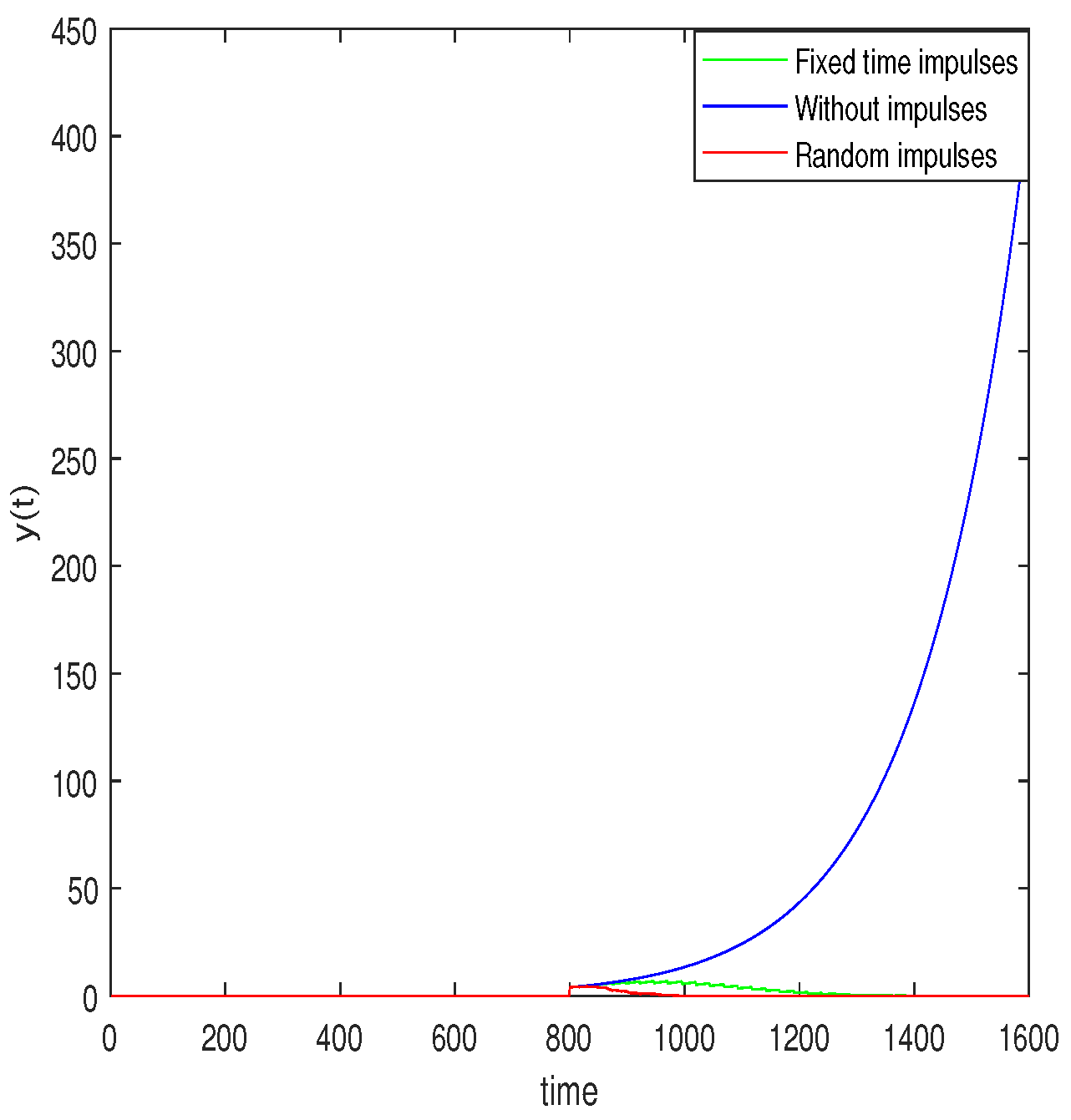
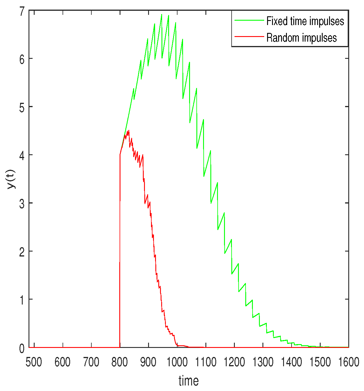
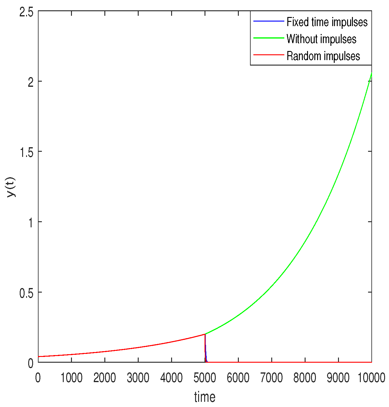
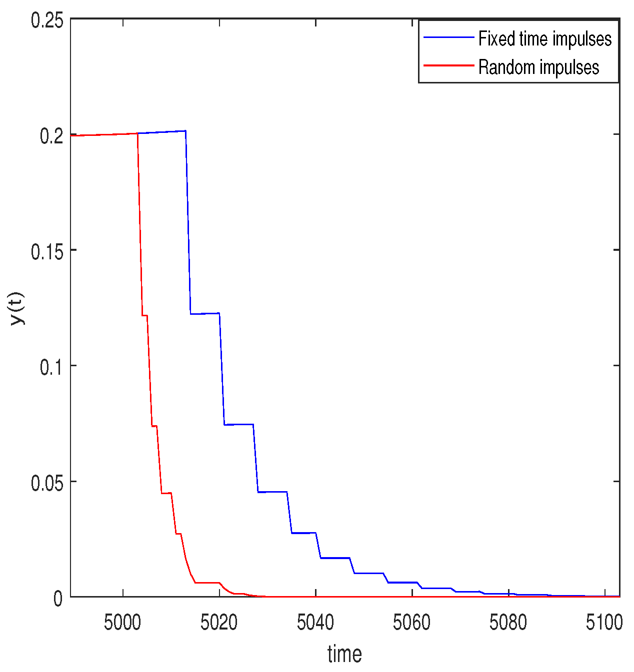
4. Example

In this part, we shall verify examples to analyze our theorems by using random impulses.

Example 1.

Consider the RIIDDE

$$\begin{array}{ccc}\hfill \dot{y}\left(t\right)& =& \left(\frac{1}{4}{e}^{-0.2t}+1\right)y\left(t\right)-2{\int }_{-\infty }^0{e}^{2\theta -0.1t}y(t+\theta )d\theta ,{\xi }_m^{{}^{\prime }}<t<{\xi }_{m+1}^{{}^{\prime }},t\ge t_0,\hfill \\ \hfill y\left({\xi }_m^{{}^{\prime }}\right)& =& \sqrt{w_m}y\left({\xi }_m^{{}^{\prime }-}\right),m=1,2,\dots ,\hfill \\ \hfill y\left(\theta \right)& =& \varphi \left(\theta \right),\theta \le t_0,\hfill \end{array}$$

(23)

where

$$\begin{array}{c}\hfill \varphi \left(\theta \right)=\left\{\begin{array}{c}0,\theta \in (-\infty ,0),\hfill \\ 4,\theta =0.\hfill \end{array}\right.\end{array}$$

Let $\mathcal{M}=4, h\left(s\right)=\frac{9}{4}$, $\mu =1$, $\kappa =0.9$, $\lambda =0.2$, $w_m=e^{-\frac{1}{5}t}$ and impulse arrival rate $\gamma =0.2$. Then, we choose the Lyapunov function $W\left(t\right)=y^2\left(t\right)$, suppose $t_0=0$, from the Corollary 1, we get $3e^{0.1t}\left|y\left(t\right)\right|>\left|y(t+\theta )\right|$. Hence,

$$\begin{array}{ccc}\hfill D^{+}W\left(t\right)& =& 2y\left(t\right)\left[\left(\frac{1}{4}{e}^{-0.2t}+1\right)y\left(t\right)-2{\int }_{-\infty }^0{e}^{2\theta -0.1t}y(t+\theta )d\theta \right]\hfill \\ & \le & -2y^2\left(t\right)\left[-\left(\frac{1}{4}{e}^{-0.2t}+1\right)+2{\int }_{-\infty }^0{e}^{2\theta -0.1t}d\theta 3e^{0.1t}\right]\hfill \\ & \le & -2y^2\left(t\right)\left[1.75\right]\hfill \\ & \le & -q{y}^2\left(t\right)=-qW\left(t\right),\hfill \end{array}$$

where $q=3.5$. By condition, we get ${\mu }^{{}^{\prime }}q-ln\mathcal{M}>\lambda {\tau }^{{}^{\prime }}$; then, we can write ${\tau }^{{}^{\prime }}<10.5685$. In addition, we have

$$\begin{array}{c}\hfill W\left({\xi }_m^{{}^{\prime }}\right)=y^2\left({\xi }_m^{{}^{\prime }}\right)=w_m{y}^2\left({\xi }_m^{{}^{\prime }-}\right)=w_{m}W\left({\xi }_m^{{}^{\prime }-}\right).\end{array}$$

Therefore, system (23) is mean square exponentially stable at the origin by Corollary 1; see the comparative results Figure 1 and Figure 2.

Example 2.

Consider the RIIDDE

$$\begin{array}{ccc}\hfill \dot{y}\left(t\right)& =& \left(\frac{1}{12}{e}^{-0.2t}+\frac{1}{4}\right)y\left(t\right)-\frac{1}{9}{\int }_{-\infty }^0,e^{\theta -0.2t}y(t+\theta )d\theta ,{\xi }_m^{{}^{\prime }}<t<{\xi }_{m+1}^{{}^{\prime }},t\ge t_0,\hfill \\ \hfill y\left({\xi }_m^{{}^{\prime }}\right)& =& \sqrt{w_m}y\left({\xi }_m^{{}^{\prime }-}\right),m=1,2,\dots ,\hfill \\ \hfill y\left(\theta \right)& =& \varphi \left(\theta \right),\theta \le t_0,\hfill \end{array}$$

(24)

where $\varphi \left(\theta \right)=0.2e^{0.2\theta }$. Consider $w_m=\frac{1}{e}$, $\kappa =0.5$, $\lambda =0.4$, and impulse arrival rate $\gamma =0.4$. We choose the Lyapunov function $W\left(t\right)=y^2\left(t\right)$, suppose $t_0=0$, from the Corollary 2, we get $\sqrt{e}{e}^{0.2t}\left|y\left(t\right)\right|>\left|y(t+\theta )\right|$. Hence,

$$\begin{array}{ccc}\hfill D^{+}W\left(t\right)& =& 2y\left(t\right)\left[\left(\frac{1}{12}{e}^{-0.2t}+\frac{1}{4}\right)y\left(t\right)-\frac{1}{9}{\int }_{-\infty }^0{e}^{\theta -0.2t}y(t+\theta )d\theta \right]\hfill \\ & \le & 2y\left(t\right)\left[\left(\frac{1}{12}{e}^{-0.2t}+\frac{1}{4}\right)y\left(t\right)-\frac{1}{9}{\int }_{-\infty }^0{e}^{\theta -0.2t}\left|y(t+\theta )\right|d\theta \right]\hfill \\ & \le & 2y^2\left(t\right)\left[\left(\frac{1}{12}{e}^{-0.2t}+\frac{1}{4}\right)-\frac{1}{9}{\int }_{-\infty }^0{e}^{s-0.2t}\sqrt{e}{e}^{0.2t}\right]\hfill \\ & \le & 2\left[\frac{1}{12}+\frac{1}{4}+\frac{\sqrt{e}}{9}\right]y^2\left(t\right)=qW\left(t\right),\hfill \end{array}$$

where $q=2\left[\frac{1}{12}+\frac{1}{4}+\frac{\sqrt{e}}{9}\right]$. By condition, $q{\tau }^{{}^{\prime }}+\lambda {\tau }^{{}^{\prime }}<ln\left(e\right)$, we get ${\tau }^{{}^{\prime }}<0.6978$. In addition, we have

$$\begin{array}{c}\hfill W\left({\xi }_m^{{}^{\prime }}\right)=y^2\left({\xi }_m^{{}^{\prime }}\right)=w_m{y}^2\left({\xi }_m^{{}^{\prime }-}\right)=w_{m}W\left({\xi }_m^{{}^{\prime }-}\right).\end{array}$$

Therefore, system (24) is mean square exponentially stable at the origin by Corollary 2; see the comparative results Figure 3 and Figure 4.

Remark 6.

The above two examples show that the unstable system can be exponentially stabilized by using the random impulses. Moreover, Figure 2 and Figure 4 represent the comparative results between fixed and random time impulses.

5. Conclusions

In this paper, we obtained several sufficient conditions for exponential stability and weakly exponential stability of RIIDDS by using the Lyapunov function and Razumikhin technique. Furthermore, we showed that random impulses are fast convergence compared with the fixed time impulses. Thus, we conclude that the random impulses are a better way to stabilize the various unstable differential systems in the future.

References

- Lakshmikantham, V.; Simeonov, P.S. Theory of Impulsive Differential Equations; World Scientific: Singapore, 1989; Volume 6. [Google Scholar]
- Samoilenko, A.M.; Perestyuk, N. Impulsive Differential Equations; World Scientific: Singapore, 1995. [Google Scholar]
- Liu, B.; Liu, X.; Teo, K.L.; Wang, Q. Razumikhin-type theorems on exponential stability of impulsive delay systems. Ima J. Appl. Math. 2006, 71, 47–61. [Google Scholar] [CrossRef]
- Liu, X.; Wang, Q. The method of lyapunov functionals and exponential stability of impulsive systems with time delay. Nonlinear Anal. Theory Methods Appl. 2007, 66, 1465–1484. [Google Scholar] [CrossRef]
- Yang, D.; Shen, J.; Zhou, Z.; Li, X. State-dependent switching control of delayed switched systems with stable and unstable modes. Math. Methods Appl. Sci. 2018, 41, 6968–6983. [Google Scholar] [CrossRef]
- Yang, X.; Li, X.; Xi, Q.; Duan, P. Review of stability and stabilization for impulsive delayed systems. Math. Biosci. Eng. 2018, 15, 1495–1515. [Google Scholar] [CrossRef] [PubMed]
- Zhang, X.; Han, X.; Li, X. Design of hybrid controller for synchronization control of chen chaotic system. J. Nonlinear Sci. Apl. 2017, 10, 3320–3327. [Google Scholar] [CrossRef][Green Version]
- Li, X.; Shen, J.; Rakkiyappan, R. Persistent impulsive effects on stability of functional differential equations with finite or infinite delay. Appl. Math. Comput. 2018, 329, 14–22. [Google Scholar] [CrossRef]
- Yang, T. Impulsive control. IEEE Trans. Autom. Control. 1999, 44, 1081–1083. [Google Scholar] [CrossRef]
- Yang, Z.; Xu, D. Stability analysis and design of impulsive control systems with time delay. IEEE Trans. Autom. Control. 2007, 52, 1448–1454. [Google Scholar] [CrossRef]
- Kayar, Z.; Zafer, A. Lyapunov-type inequalities for nonlinear impulsive systems with applications. Elec. J. Qual. Theory Differ. Equ. 2016, 27, 1–13. [Google Scholar] [CrossRef]
- Li, X.; Ding, Y. Razumikhin-type theorems for time-delay systems with persistent impulses. Syst. Control. Lett. 2017, 107, 22–27. [Google Scholar] [CrossRef]
- Li, X.; Wu, J. Stability of nonlinear differential systems with state-dependent delayed impulses. Automatica 2016, 64, 63–69. [Google Scholar] [CrossRef]
- Li, X.; Yang, X.; Huang, T. Persistence of delayed cooperative models: Impulsive control method. Appl. Math. Comput. 2019, 342, 130–146. [Google Scholar] [CrossRef]
- Liu, X.; Ballinger, G. Uniform asymptotic stability of impulsive delay differential equations. Comput. Math. Appl. 2001, 41, 903–915. [Google Scholar] [CrossRef]
- Zhang, X.; Li, X.; Song, S. Effect of delayed impulses on input-to-state stability of nonlinear systems. Automatica 2017, 76, 378–382. [Google Scholar]
- Anguraj, A.; Vinodkumar, A. Existence, uniqueness and stability results of random impulsive semilinear differential systems. Nonlinear Anal. Hybrid Syst. 2010, 4, 475–483. [Google Scholar] [CrossRef]
- Wu, S. Exponential stability of random impulsive differential systems. Acta Math. Sci. 2005, 25, 789–798. [Google Scholar]
- Agarwal, R.; Hristova, S.; O’Regan, D. Exponential stability for differential equations with random impulses at random times. Adv. Differ. Equ. 2013, 1, 372. [Google Scholar] [CrossRef]
- Agarwal, R.; Hristova, S.; Kopanov, P.; O’Regan, D. Impulsive differential equations with gamma distributed moments of impulses and p-moment exponential stability. Acta Math. Sci. 2017, 37, 985–997. [Google Scholar] [CrossRef]
- Anguraj, A.; Vinodkumar, A.; Malar, K. Existence and stability results for random impulsive fractional pantograph equations. Filomat 2016, 30, 3839–3854. [Google Scholar] [CrossRef]
- Caraballo, T.; Cortes, J.; Navarro-Quiles, A. Applying the random variable transformation method to solve a class of random linear differential equation with discrete delay. Appl. Math. Comput. 2019, 356, 198–218. [Google Scholar] [CrossRef]
- Gikhman, I.I.; Skorokhod, A.V. Stochastic differential equations. In The Theory of Stochastic Processes III; Springer: Berlin/Heidelberg, Germany, 2007; pp. 113–219. [Google Scholar]
- Gowrisankar, M.; Mohankumar, P.; Vinodkumar, A. Stability results of random impulsive semilinear differential equations. Acta Math. Sci. 2014, 34, 1055–1071. [Google Scholar] [CrossRef]
- Shaikhet, L. Lyapunov Functionals and Stability of Stochastic Functional Differential Equations; Springer Science & Business Media: Berlin/Heidelberg, Germany, 2013. [Google Scholar]
- Vinodkumar, A.; Anguraj, A. Existence of random impulsive abstract neutral non-autonomous differential inclusions with delays. Nonlinear Anal. Hybrid Syst. 2011, 5, 413–426. [Google Scholar] [CrossRef]
- Vinodkumar, A.; Malar, K.; Gowrisankar, M.; Mohankumar, P. Existence, uniqueness and stability of random impulsive fractional differential equations. Acta Math. Sci. 2016, 36, 428–442. [Google Scholar] [CrossRef]
- Vinodkumar, A.; Senthilkumar, T.; Li, X. Robust exponential stability results for uncertain infinite delay differential systems with random impulsive moments. Adv. Differ. Equ. 2018, 1, 39. [Google Scholar] [CrossRef]
- Wu, S.; Guo, X.; Zhou, Y. P-moment stability of functional differential equations with random impulses. Comput. Math. Appl. 2006, 52, 1683–1694. [Google Scholar] [CrossRef]
© 2019 by the authors. Licensee MDPI, Basel, Switzerland. This article is an open access article distributed under the terms and conditions of the Creative Commons Attribution (CC BY) license (http://creativecommons.org/licenses/by/4.0/).
Share and Cite
Li, X.; Vinodkumar, A.; Senthilkumar, T. Exponential Stability Results on Random and Fixed Time Impulsive Differential Systems with Infinite Delay. Mathematics 2019, 7, 843. https://doi.org/10.3390/math7090843
Li X, Vinodkumar A, Senthilkumar T. Exponential Stability Results on Random and Fixed Time Impulsive Differential Systems with Infinite Delay. Mathematics. 2019; 7(9):843. https://doi.org/10.3390/math7090843
Chicago/Turabian StyleLi, Xiaodi, A. Vinodkumar, and T. Senthilkumar. 2019. "Exponential Stability Results on Random and Fixed Time Impulsive Differential Systems with Infinite Delay" Mathematics 7, no. 9: 843. https://doi.org/10.3390/math7090843
APA StyleLi, X., Vinodkumar, A., & Senthilkumar, T. (2019). Exponential Stability Results on Random and Fixed Time Impulsive Differential Systems with Infinite Delay. Mathematics, 7(9), 843. https://doi.org/10.3390/math7090843