Tuning Multi-Objective Evolutionary Algorithms on Different Sized Problem Sets

Abstract

Multi-Objective Evolutionary Algorithms (MOEAs) have been applied successfully for solving real-world multi-objective problems. Their success can depend highly on the configuration of their control parameters. Different tuning methods have been proposed in order to solve this problem. Tuning can be performed on a set of problem instances in order to obtain robust control parameters. However, for real-world problems, the set of problem instances at our disposal usually are not very plentiful. This raises the question: What is a sufficient number of problems used in the tuning process to obtain robust enough parameters? To answer this question, a novel method called MOCRS-Tuning was applied on different sized problem sets for the real-world integration and test order problem. The configurations obtained by the tuning process were compared on all the used problem instances. The results show that tuning greatly improves the algorithms’ performance and that a bigger subset used for tuning does not guarantee better results. This indicates that it is possible to obtain robust control parameters with a small subset of problem instances, which also substantially reduces the time required for tuning.

1. Introduction

Setting control parameters of Evolutionary Algorithms (EAs) remains one of the biggest challenges in evolutionary computation. Control parameters have a great impact on the performance of Evolutionary Algorithms; a poor setting can even make it impossible to solve the given problem at hand [1]. Tuning is performed in order to find good control parameters, and is known as a parameter tuning problem [2]. Tuning plays an important role in evolutionary algorithms: not only does it improve the algorithms’ performance, but it also enables us to perform a fair comparison between different algorithms [3]. However, tuning is very time-consuming and, therefore, we cannot always afford to tune an EA for each given instance of the problem individually even though tuning is carried out off-line. To avoid tuning on individual problem instances, it can be carried-out on only a subset of instances. This provides us with robust control parameters, making the tuned algorithm a generalist [4]. However, we do not know how many instances of the problem should be used in the tuning process to produce robust control parameters, or if it is even possible.

To answer this question, we performed tuning with different sized sets of problem instances (problem sets). The tuning was conducted with a novel method, which uses a Chess Rating System [3], adapted for Multi-Objective Optimization and is called MOCRS-Tuning. MOCRS-Tuning uses a meta-evolutionary approach to find the best configuration (control parameters) for the given MOEA. The search for the best configuration is guided by a self-adaptive Differential Evolution (jDE) [5]. Since it is self-adaptive, we do not need to deal with additional parameters in the tuning process. Each configuration of the MOEA is evaluated using a Chess Rating System with a Quality Indicator Ensemble (CRS4MOEA/QIE) [6]. The Chess Rating System treats each configuration as a player and each comparison between two configurations as a game. In a game, approximation sets of two competing configurations are evaluated with a Quality Indicator (QI) and compared. A game is played between each player for every problem evaluated with different QIs. Afterwards, the player’s rating is calculated using the resulting game outcomes. The rating acts as the configuration’s fitness. Because different QIs are used in the assessment, the rating (fitness) reflects different aspects of quality [7]. The same Chess Rating System is incorporated in the Evolutionary Algorithms Rating System (EARS) framework [8]. The EARS framework was used to compare the configurations obtained by tuning an MOEA on differently sized problem sets. The tuning was performed on a real-world problem called Integration and Testing Order (ITO) for which MOEAs have been shown suitable to solve effectively [9,10]. A real-world problem will show the impact of tuning better, since MOEAs with default control parameters perform relatively well on benchmark problems [11].

The remainder of the paper is organized as follows. The most relevant related work is presented in Section 2. Section 3 describes the ITO problem. In Section 4, the Chess Rating System for evolutionary algorithms is described. Section 5 describes the applied tuning method. The execution of the experiment is presented in Section 6. Results are presented and discussed in Section 7. Section 8 concludes the paper.

2. Related Work

The issue of setting control parameters of EAs has been present since their conception. Consequently, a significant amount of research has been done in the field of tuning evolutionary algorithms. In the literature, numerous different tuning methods have been proposed [12,13,14,15,16,17], and many studies on tuning have been conducted [1,18,19]. Below follows a brief description of the most relevant related works.

Veček et al. [3] proposed a novel tuning method for single-objective EAs, which uses a Chess Rating System called CRS-Tuning. The method was compared to two well-established tuning methods, F-Race [12] and Estimation and Value Calibration of Evolutionary Algorithm Parameters (REVAC) [13]. They concluded that all three methods showed strengths and weaknesses in different areas, and the results of the CRS-Tuning method were comparable with the results found by the other two methods. The configurations found with CRS-Tuning were, in most cases, amongst the best when compared using the Friedman ranking. In this study, we adapted the CRS-Tuning method for MOEAs using an ensemble of QIs.

Smit and Eiben [4] used REVAC to tune an EA to a set of problems (generalist) to obtain robust control parameters. They compared the generalist with the supposedly robust conventional values and found great differences. The results also show that default settings of control parameters might be far from optimal, even if they are meant to be robust. Our work shares some similarities, but was extended to multi-objective problems. In addition, our experiments were performed on real-world problems, which are not explored in detail, such as benchmark problems. This gives a better insight into the robustness of control parameters.

Arcuri and Fraser [11,20] performed the largest empirical analysis to date on parameter tuning in Search-Based Software Engineering (SBSE). Their analysis includes data from more than a million experiments. In their experiments, they focused on test data generation for object-oriented software using the EvoSuite tool. The results showed that tuning has a big impact on the algorithm’s performance. They also provided guidelines on how to handle parameter tuning. In this study, we also performed tuning on a software engineering problem. However, in our case, the problem is multi-objective. In addition, because of the scale of their experiments, they limited the tuning process to a predefined set of values for each control parameter.

Zaefferer et al. [21] also performed tuning on a real-world multi-objective problem. They tuned two algorithms with Sequential Parameter Optimization (SPO) [15] for the cyclone (dust separator) optimization problem. The algorithms were tuned under two different specifications. In the first case, the algorithms are tuned to require as few function evaluations as possible for a specified target hypervolume value. In the second case, a very small budget was imposed, and the algorithms were tuned for a best performance with respect to hypervolume. In our case, we used maximum evaluations as the stopping criterion. In addition, more problem instances were considered, in order to observe the impact on the performance of MOEAs. Furthermore, we considered more quality indicators for better evaluation.

3. Integration and Testing Order

Software testing is an important activity in the Software Development Life Cycle (SDLC). It is the process of finding defects in the software under development. Software testing also helps us to identify errors, gaps or missing requirements [22]. It can be done manually or using automated tools at different levels: unit testing, integration testing, system testing, and acceptance testing. Testing shows a presence of defects, and not the absence of defects. Hence, it is often combined with static and dynamic analysis of software (e.g., [23,24]). One common problem in software testing is determining the order in which units need to be integrated and tested. The order is important since it affects the design of test cases, the order in which units are developed, the order in which interaction problems between units are detected and the number of required stubs. A stub is a dummy component that simulates the functions of a real component (unit) [25]. Stubs are required when a unit depends on another unit, which is not yet developed or tested. The construction of stubs is very error-prone and expensive. The goal of the integration and testing order problem is to determine an order that minimizes the stubbing cost [10]. The stubbing process is influenced by different objectives, which makes MOEAs suitable for solving the ITO problem [9,10].

The two objectives of the problem that have to be minimized are the number of emulated attributes and methods in the stub. An instance of the ITO problem is a system. In our experiments, we used eight real-world systems:

• MyBatis (http://www.mybatis.org/mybatis-3/) is a first class persistence framework with support for custom SQL, stored procedures and advanced mappings.
• AJHSQLDB (HyperSQL DataBase) (https://sourceforge.net/projects/ajhsqldb/) is the aspect-oriented version of the leading relational database software written in Java.
• BCEL (Byte Code Engineering Library) (https://commons.apache.org/proper/commons-bcel/) is intended to give users a convenient way to analyze, create, and manipulate (binary) Java class files.
• JHotDraw (http://www.jhotdraw.org/) is a Java framework for technical and structured graphics.
• HealthWatcher (http://www.aosd-europe.net/) collects and manages public health related to complaints and notifications.
• JBoss (http://jbossas.jboss.org/downloads) is a Java application server.
• AJHotDraw (http://ajhotdraw.sourceforge.net/) is an aspect-oriented refactoring of JHotDraw.
• TollSystems (http://www.comp.lancs.ac.uk/greenwop/tao) is a concept proof for automatic charging of toll on roads and streets.

It should be noted that the systems used are just examples of problem instances for the ITO problem and do not require any additional software in the execution environment. Information about the systems, such as the number of dependencies, classes, aspects, and Lines of Code (LOC), is given in

Table 1. Eight real-world problem instances (systems) for the ITO problem used in the experiments.

Num	Name	Dependencies	Classes	Aspects	LOC
1	AJHotDraw	1592	290	31	18,586
2	AJHSQLDB	1338	276	15	68,550
3	MyBatis	1271	331	-	23,535
4	JHotDraw	809	197	-	20,273
5	JBoss	367	150	-	8434
6	HealthWatcher	289	95	22	5479
7	BCEL	289	45	-	2999
8	TollSystems	188	53	24	2496

.

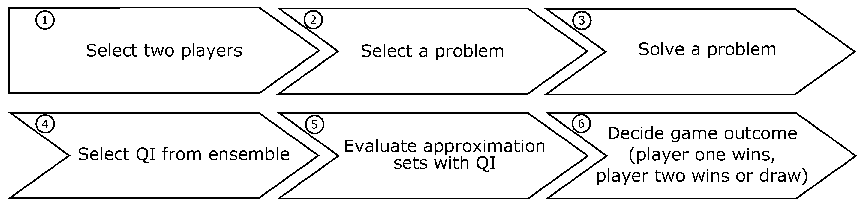
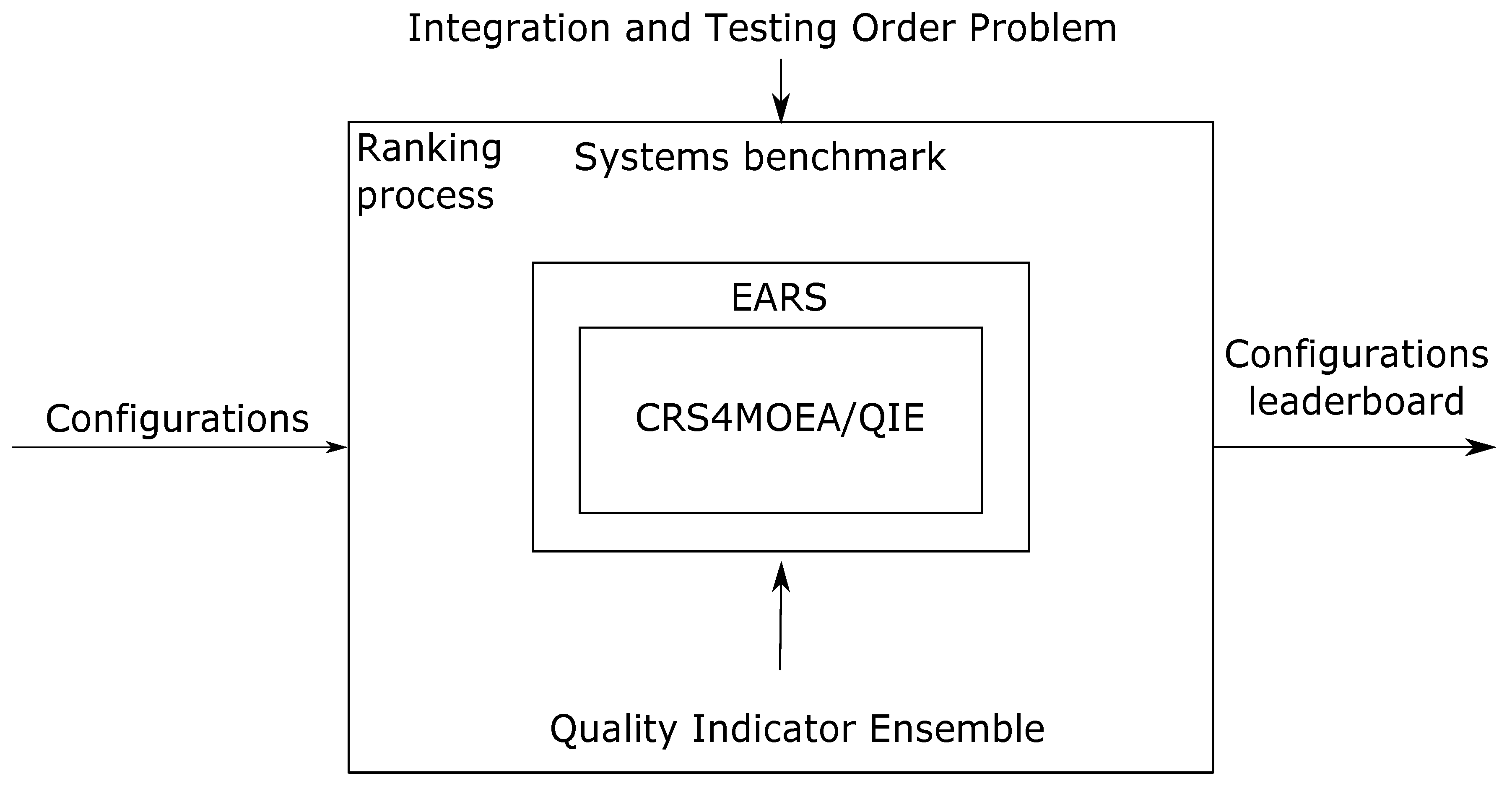
4. Chess Rating System for Evolutionary Algorithms

A chess rating system with a quality indicator ensemble (CRS4MOEA/QIE) is a novel method for comparing MOEAs. We used the chess rating system to compare the different configurations of MOEAs obtained by tuning. The idea behind the ensemble is that different aspects of quality are considered since a single QI cannot reliably assess all aspects at once [26]. To ensure that all aspects of quality are considered, we chose a diverse set of QIs [6]. Of course, a user could tailor the ensemble for his needs. CRS4MOEA/QIE uses the Glicko-2 system [27] to estimate a player’s skill level. To rank players, they need to participate in a tournament. The style of the tournament is round-robin where each player plays against all other players. In the case of CRS4MOEA/QIE, players are different MOEAs and/or different configurations thereof. A tournament consists of a series of games. Unlike classical chess where only one game is played between two players, in our case, a game is played for each given problem. In addition, in CRS4MOEA/QIE, a tournament is conducted with multiple independent runs where multiple games are played for the same problem. Figure 1 shows how a single game between two players is conducted. In the first step, two players participating in the tournament are selected. In the next step, a problem is selected. The two players have to solve the same problem with the same stopping criterion. After they reach the stopping criterion, they return an approximation set. In Step 4, a quality indicator from the ensemble is selected and is used to evaluate the two approximations. In the last step, the two values returned by the QI are compared, and the outcome of the game is decided. The outcomes of the games are used to update each player’s rating R and rating deviation $RD$[27]. New (unrated) players have their starting rating set to 1500 and their $RD$ to 350. A player’s rating increases if he plays better than expected. Therefore a higher rating indicates a better player. However, if he plays worse than expected, his rating decreases. In both cases, the amount by which the rating increases/decreases depends on the player’s rating as well as the opponent’s rating. The rating deviation measures the accuracy of a player’s rating. A smaller $RD$ is desired since it indicates a more reliable rating. In our experiments, CRS4MOEA/QIE was used in the tuning process to evaluate different configurations and to compare the different configurations obtained by tuning.

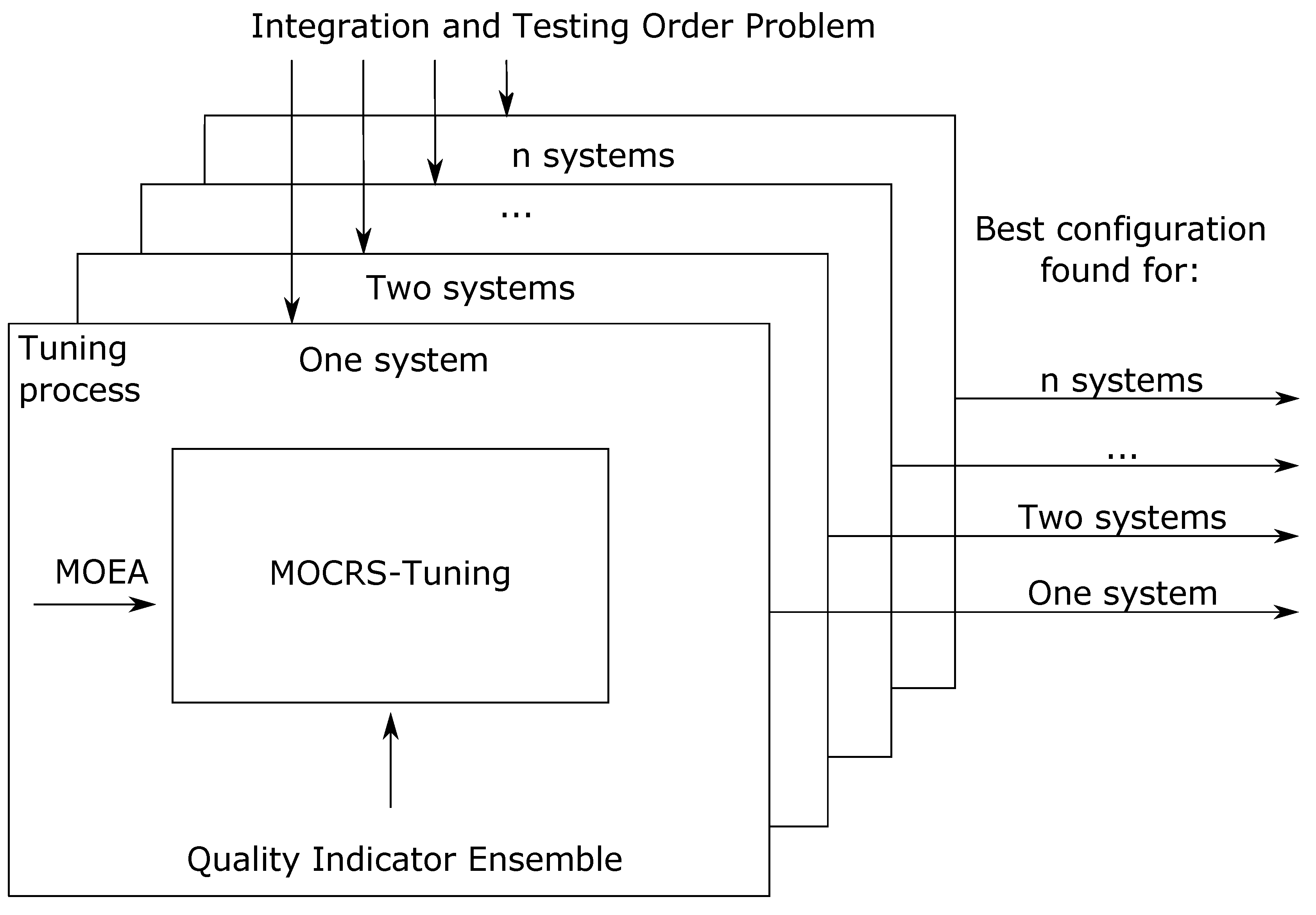
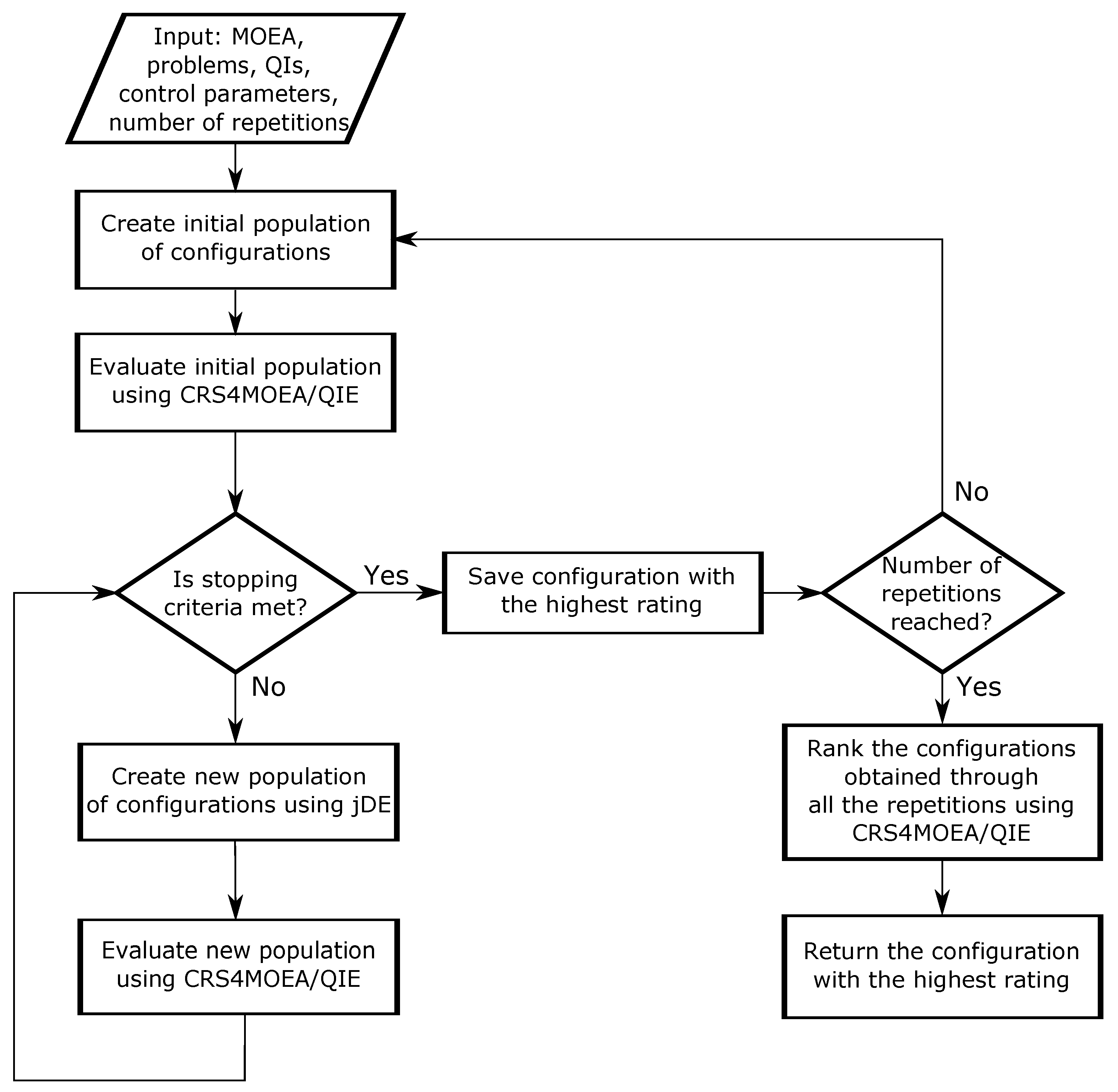
5. MOCRS-Tuning Method

The tuning method (MOCRS-Tuning) used in our experiments is shown in Figure 2. MOCRS-Tuning uses a meta-evolutionary approach for parameter tuning. The input parameters are the MOEA to be tuned, the set of problems (in our case systems) for which it will be tuned, QIs used to evaluate and compare obtained results, control parameters to be tuned, and the number of repetitions of the tuning process. First, an initial population of configurations is created for the given MOEA. For each configuration, the control parameters are generated randomly within the given lower and upper bounds. Before the main loop starts, the generated population containing different configurations is evaluated using CRS4MOEA/QIE. The whole population participates in the tournament and, when it is completed, each configuration obtains its rating R, which represents its fitness. The tuning process takes place in the main loop and is guided by jDE and CRS4MOEA/QIE. First, an offspring population of new configurations is generated with jDE’s search mechanisms. Each newly generated solution plays in a tournament with the old population and is evaluated with CRS4MOEA/QIE. In the next step, ratings of the newly generated solutions are compared with their parents. If the offspring solution has a higher rating than its parent, it is added to the new population; otherwise, its parent is added. In the case that the new population has new solutions, their ratings need to be recalculated since the individuals rating is dependant on the whole population. If no new solutions exist in the new population, this step can be skipped. The process is repeated until the stopping criterion is met. The configuration with the highest rating is saved for later. The process is repeated for the given number of repetitions. A completely new initial population is generated in each repetition. When the number of repetitions is reached, one last tournament is performed. In the tournament, the best configuration of each repetition is evaluated using CRS4MOEA/QIE. The configuration with the highest rating is returned.

6. Experiment

In the experiment, MOCRS-Tuning was performed on different sized problem sets. Figure 3 shows how the tuning was conducted. First, we gave MOCRS-Tuning only one system for the ITO problem as input. The output was the best configuration found for the given system. Another system was added, and the tuning process was performed again. This was repeated until all eight system were used. This resulted in eight configurations, each tuned for the given problem set.

Table 2. System sets used and the approximate tuning time.

Run	Systems Included	Tuning Time (h)
1	4	14
2	4, 3	30
3	4, 3, 7	35
4	4, 3, 7, 5	37
5	4, 3, 7, 5, 1	41
6	4, 3, 7, 5, 1, 8	51
7	4, 3, 7, 5, 1, 8, 2	56
8	4, 3, 7, 5, 1, 8, 2, 6	63

shows which systems were used in the eight sets (column Systems included). The numbers correspond to the systems in Table 1 (column Num). We also added the approximate tuning time. The tuning was performed on a computer with an Intel(R) Core(TM) i7-4790 3.60 GHz CPU and 16 GB of RAM. As can be seen, the tuning process was very time-consuming, taking approximately 63 h on eight systems. Table 1 nicely shows our motivation. We wanted to test whether this tuning cost contributes to overall results or will we receive similar results with default control parameters. Besides, we wanted to investigate how many systems are enough to include in the tuning process for this particular real-world (ITO) problem.

For comparison of the different configurations, we performed ranking using the EARS framework. The ranking process is shown in Figure 4. As input, we give it the configurations we want to rank and the problems (systems) on which they will be compared. When the tournament is completed, EARS outputs a leaderboard consisting of ranks, ratings and rating deviations of all competing players (configurations). In the experiment, the ranking was performed in two different scenarios. Firstly, it was performed on configurations obtained with each repetition of the tuning process in order to see the robustness of the method. This was done for each problem set. Secondly, the ranking was performed on the best configurations for each problem set returned by MOCRS-Tuning and a default configuration. The ranking was performed on each system individually.

Experimental Settings

In the experiment, MOCRS-Tuning was applied to $MOEA/D$ [28], which was continuously proven effective for solving multi-objective problems. The problem sets contained different numbers of previously mentioned systems for the ITO problem. For each system, the stopping criterion was set to 60,000 fitness evaluations [9,29]. The quality indicator ensemble contained five different QIs:

• Inverted Generational Distance ($IG{D}^{+}$) [30]
• Hypervolume ($HV$) [31]
• $R2$ [32]
• Maximum Spread ($MS$) [33]
• Unary additive $ϵ$-indicator ($I_{ϵ+}$) [26]

The number of repetitions in MOCRS-Tuning was set to 8. The control parameters which underwent the tuning process were population size, crossover probability, and mutation probability. MOCRS-Tuning accepts upper and lower bounds for control parameters in order to limit the search space. Therefore, the lower and upper bounds for population size were set to 10 and 500, respectively. For mutation and crossover probability, we set the lower and upper bound to 0.1 and 1.0, respectively. The number of configurations (population size) for jDE was set to 20. The stopping criterion was set to 30 generations. In the ranking process (Figure 4), the number of independent runs of the tournament was set to 15.

7. Results and Discussion

MOCRS-Tuning saves the best configuration in each repetition and, at the end, returns the best one amongst all saved configurations. To observe the robustness of the tuning method, we performed ranking on the eight saved configurations for each problem set. We used the ranking process (Figure 4), where the input was the eight configurations (Table 2), and the benchmark set contained the same systems for which they were tuned. Using the ratings and $RD$s of the obtained configurations, we plotted their Rating Intervals (RIs) also known as confidence intervals. In our case, we used the 95% confidence level, which, according to the three-sigma rule [34], means that we are 95% confident that the rating R lies in the interval $\left[R-2RD,R+2RD\right]$. If we compare two rating intervals and they do not overlap, then the two configurations are significantly different. The rating intervals of the eight configurations for each problem set are shown in Figure 5. Each RI has a label showing the values of the obtained control parameters. Significant differences occurred only in the case where one system was used in the tuning. The best two configurations (Figure 5a) top) performed significantly better than the two worst (Figure 5a) bottom). In the rest of the cases, where more than one system was used in the tuning process, there are no significant differences between configurations. This indicates that the tuning method is very robust.

In the next scenario, we took the best configuration for each problem set and performed the ranking process on the eight systems. In this case, we also added the default configuration of $MOEA/D$ based on the authors’ recommendation and source code from the jMetal framework [35]. The default value for population size was set to 100, crossover probability to 1.0 and mutation probability to 0.2. Figure 6 shows the Rating Intervals of all configurations ranked on all eight systems. We can observe that the tuned configurations performed significantly better than the default configuration in most cases (Figure 6), proving that tuning can improve the algorithms’ performance greatly. There are significant differences between tuned configurations only in the case of system AJHSQLDB. One would expect that the configuration tuned on one system would perform the best on the system it was tuned. However, if we look at rating intervals for JHotDraw, we can see that this is not the case. One explanation for this phenomenon is that all other configurations also contained this system when they were tuned. Another false assumption is that tuned configuration on all eight systems will outperform others in all benchmarks. On the contrary, only for two systems this was the case (MyBatis and AJHSQLDB, see Figure 6), which is a confirmation of the NFL theorem.

One of the more interesting findings is that there are few significant differences amongst tuned configurations (e.g., AJHSQLDB). This means that the problem set size does not have such a big impact on the algorithms performance as tuning itself. We can conclude from the results that tuning is important and that tuning for each problem individually does not guarantee good performance. When conducting tuning, the domain of the problem for which algorithms are tuned play an important role. In addition, it is hard to determine the best number of problems used for tuning in order to get the best performance.

8. Conclusions

In this study, we investigated how the size of the problem set impacts the tuning of MOEAs. The tuning was performed with MOCRS-Tuning, which uses a jDE and a chess rating system with a quality indicator ensemble to find the best configuration for the given MOEA. The tuning was conducted on different sized problem sets containing systems, which represent instances of the real-world ITO problem. The obtained configurations were compared using the EARS framework. The experiments were based on a chess rating system, which we showed to be equivalent to NHST and the conclusions were comparable [3]. However, the approach can be performed with other tuning methods. It is also not limited to a specific MOEA or a specific set of quality indicators. The results show that the tuning method is robust no matter how many systems are used in the tuning process. From the comparison of the different configurations, we see that tuning has a great impact on the performance. We also concluded that tuning on individual problems is not always worth it since it is very time-consuming and does not guarantee better results. Robust control parameters can be obtained even on a small set of problem instances, since there were no significant differences amongst tuned configurations in most cases. Using the novel tuning method for multi-objective algorithms called MOCRS-Tuning, we demonstrated that good control parameters with a small problem set (number of systems) can be obtained. With MOCRS-Tuning, the total tuning time required can be substantially reduced, making it more practical and feasible.

For future work, we would like to perform tuning on additional MOEAs to investigate the novel method better. One additional aspect we would also so like to consider in our future experiments is the number of objectives. We would like to see how problems with higher numbers of objectives affect the tuning process. Another possible threat to validity is the design of the tuning process. In our experiment, we integrated eight different systems in a random order (see Table 2). We are interested in how a different order would affect the performance of the configurations. The connected idea is to carefully form system subsets. We can combine them based on certain characteristics of the problem. Another goal is to use other real-world problems and observe how the configurations obtained on one type of problem perform on another.

References

1. Eiben, A.E.; Smit, S.K. Parameter tuning for configuring and analyzing evolutionary algorithms. Swarm Evol. Comput. 2011, 1, 19–31. [Google Scholar] [CrossRef] [Green Version]
2. Karafotias, G.; Hoogendoorn, M.; Eiben, Á.E. Parameter control in evolutionary algorithms: Trends and challenges. IEEE Trans. Evol. Comput. 2015, 19, 167–187. [Google Scholar] [CrossRef]
3. Veček, N.; Mernik, M.; Filipič, B.; Črepinšek, M. Parameter tuning with Chess Rating System (CRS-Tuning) for meta-heuristic algorithms. Inf. Sci. 2016, 372, 446–469. [Google Scholar] [CrossRef]
4. Smit, S.K.; Eiben, A. Parameter tuning of evolutionary algorithms: Generalist vs. specialist. In European Conference on the Applications of Evolutionary Computation; Springer: Berlin/Heidelberg, Germany, 2010; pp. 542–551. [Google Scholar]
5. Brest, J.; Žumer, V.; Maučec, M. Self-Adaptive Differential Evolution Algorithm in Constrained Real-Parameter Optimization. In Proceedings of the IEEE Congress on Evolutionary Computation (CEC 2006), Vancouver, BC, Canada, 16–21 July 2006; pp. 215–222. [Google Scholar]
6. Ravber, M.; Mernik, M.; Črepinšek, M. Ranking Multi-Objective Evolutionary Algorithms using a Chess Rating System with Quality Indicator ensemble. In Proceedings of the IEEE Congress on Evolutionary Computation (CEC 2017), San Sebastian, Spain, 5–8 June 2017; pp. 1503–1510. [Google Scholar]
7. Ravber, M.; Mernik, M.; Črepinšek, M. The Impact of Quality Indicators on the Rating of Multi-objective Evolutionary Algorithms. In Proceedings of the Conference on Bioinspired Optimization Methods and Their Applications (BIOMA 2016), Bled, Slovenia, 18–20 May 2016; pp. 119–130. [Google Scholar]
8. EARS—Evolutionary Algorithms Rating System (Github). 2019. Available online: https://github.com/UM-LPM/EARS (accessed on 2 August 2019).
9. Assunção, W.K.G.; Colanzi, T.E.; Vergilio, S.R.; Pozo, A. A multi-objective optimization approach for the integration and test order problem. Inf. Sci. 2014, 267, 119–139. [Google Scholar] [CrossRef]
10. Assunção, W.K.G.; Colanzi, T.E.; Pozo, A.T.R.; Vergilio, S.R. Establishing integration test orders of classes with several coupling measures. In Proceedings of the Conference on Genetic and Evolutionary Computation (GECCO 2011), Dublin, Ireland, 12–16 July 2011; pp. 1867–1874. [Google Scholar]
11. Arcuri, A.; Fraser, G. Parameter tuning or default values? An empirical investigation in search-based software engineering. Empir. Softw. Eng. 2013, 18, 594–623. [Google Scholar] [CrossRef]
12. Birattari, M.; Stützle, T.; Paquete, L.; Varrentrapp, K. A racing algorithm for configuring metaheuristics. In Proceedings of the Conference on Genetic and Evolutionary Computation (GECCO 2002), New York, NY, USA, 9–13 July 2002; Morgan Kaufmann Publishers Inc.: San Francisco, CA, USA, 2002; pp. 11–18. [Google Scholar]
13. Nannen, V.; Eiben, A.E. Relevance Estimation and Value Calibration of Evolutionary Algorithm Parameters. In Proceedings of the 20th International Joint Conference on Artifical Intelligence, Singapore, 25–28 September 2007; Morgan Kaufmann Publishers Inc.: San Francisco, CA, USA, 2007; pp. 975–980. [Google Scholar]
14. Hutter, F.; Hoos, H.H.; Stützle, T. Automatic Algorithm Configuration Based on Local Search. In Proceedings of the 22Nd National Conference on Artificial Intelligence, Vancouver, BC, Canada, 22–26 July 2007; AAAI Press: New York, NY, USA, 2007; pp. 1152–1157. [Google Scholar]
15. Bartz-Beielstein, T.; Lasarczyk, C.W.; Preuß, M. Sequential parameter optimization. In Proceedings of the IEEE Congress on Evolutionary Computation (CEC 2005), Edinburgh, UK, 2–5 September 2005; Volume 1, pp. 773–780. [Google Scholar]
16. Smit, S.K.; Eiben, A.E.; Szlávik, Z. An MOEA-based Method to Tune EA Parameters on Multiple Objective Functions. In Proceedings of the IJCCI (ICEC), Valencia, Spain, 24–26 October 2010; pp. 261–268. [Google Scholar]
17. Yuan, B.; Gallagher, M. Combining meta-EAs and racing for difficult EA parameter tuning tasks. In Parameter Setting in Evolutionary Algorithms; Springer: Berlin/Heidelberg, Germany, 2007; pp. 121–142. [Google Scholar]
18. Montero, E.; Riff, M.C.; Neveu, B. A beginner’s guide to tuning methods. Appl. Soft Comput. 2014, 17, 39–51. [Google Scholar] [CrossRef]
19. Smit, S.K.; Eiben, A.E. Comparing parameter tuning methods for evolutionary algorithms. In Proceedings of the IEEE Congress on Evolutionary Computation (CEC 2009), Trondheim, Norway, 18–21 May 2009; pp. 399–406. [Google Scholar]
20. Arcuri, A.; Fraser, G. On parameter tuning in search based software engineering. Search Based Softw. Eng. 2011, 33–47. [Google Scholar]
21. Zaefferer, M.; Breiderhoff, B.; Naujoks, B.; Friese, M.; Stork, J.; Fischbach, A.; Flasch, O.; Bartz-Beielstein, T. Tuning multi-objective optimization algorithms for cyclone dust separators. In Proceedings of the Conference on Genetic and Evolutionary Computation (GECCO 2014), Vancouver, BC, Canada, 12–16 July 2014; pp. 1223–1230. [Google Scholar]
22. Naumchev, A.; Meyer, B.; Mazzara, M.; Galinier, F.; Bruel, J.M.; Ebersold, S. AutoReq: Expressing and verifying requirements for control systems. J. Comput. Lang. 2019, 51, 131–142. [Google Scholar] [CrossRef] [Green Version]
23. Choi, W.; Kannan, J.; Babic, D. A scalable, flow-and-context-sensitive taint analysis of android applications. J. Comput. Lang. 2019, 51, 1–14. [Google Scholar] [CrossRef]
24. Tsutano, Y.; Bachala, S.; Srisa-An, W.; Rothermel, G.; Dinh, J. Jitana: A modern hybrid program analysis framework for android platforms. J. Comput. Lang. 2019, 52, 55–71. [Google Scholar] [CrossRef] [Green Version]
25. Beizer, B. Software Testing Techniques; Dreamtech Press: Delhi, India, 2003. [Google Scholar]
26. Zitzler, E.; Thiele, L.; Laumanns, M.; Fonseca, C.M.; Da Fonseca, V.G. Performance assessment of multiobjective optimizers: an analysis and review. IEEE Trans. Evol. Comput. 2003, 7, 117–132. [Google Scholar] [CrossRef] [Green Version]
27. Glickman, M.E. Example of the Glicko-2 System; Boston University: Boston, MA, USA, 2012. [Google Scholar]
28. Zhang, Q.; Li, H. MOEA/D: A multiobjective evolutionary algorithm based on decomposition. IEEE Trans. Evol. Comput. 2007, 11, 712–731. [Google Scholar] [CrossRef]
29. Guizzo, G.; Vergilio, S.R.; Pozo, A.T.; Fritsche, G.M. A multi-objective and evolutionary hyper-heuristic applied to the Integration and Test Order Problem. Appl. Soft Comput. 2017, 56, 331–344. [Google Scholar] [CrossRef] [Green Version]
30. Ishibuchi, H.; Masuda, H.; Tanigaki, Y.; Nojima, Y. Difficulties in specifying reference points to calculate the inverted generational distance for many-objective optimization problems. In Proceedings of the IEEE Symposium on Computational Intelligence in Multi-Criteria Decision-Making (MCDM), Orlando, FL, USA, 9–12 December 2014; pp. 170–177. [Google Scholar]
31. Zitzler, E.; Thiele, L. Multiobjective evolutionary algorithms: a comparative case study and the strength Pareto approach. IEEE Trans. Evol. Comput. 1999, 3, 257–271. [Google Scholar] [CrossRef] [Green Version]
32. Hansen, M.P.; Jaszkiewicz, A. Evaluating the Quality of Approximations to the Non-Dominated Set; IMM, Department of Mathematical Modelling, Technical University of Denmark: Kongens Lyngby, Denmark, 1998. [Google Scholar]
33. Yen, G.G.; He, Z. Performance metric ensemble for multiobjective evolutionary algorithms. IEEE Trans. Evol. Comput. 2014, 18, 131–144. [Google Scholar] [CrossRef]
34. Pukelsheim, F. The three sigma rule. Am. Stat. 1994, 48, 88–91. [Google Scholar]
35. Durillo, J.J.; Nebro, A.J. jMetal: A Java framework for multi-objective optimization. Adv. Eng. Softw. 2011, 42, 760–771. [Google Scholar] [CrossRef]
Figure 1. A single game in CRS4MOEA/QIE.
Mathematics 07 00824 g001
Figure 2. MOCRS-Tuning flowchart.
Mathematics 07 00824 g002
Figure 3. Experimental execution of the tuning process.
Mathematics 07 00824 g003
Figure 4. Experimental execution of the ranking process.
Mathematics 07 00824 g004
Figure 5. Rating intervals for configurations obtained from the eight repetitions within the MOCRS-Tuning process ranked on eight different problem sets. For each configuration, the control parameters population size (pop), crossover probability (cp) and mutation probability (mp) are given.
Mathematics 07 00824 g005
Figure 6. Rating intervals for the best configurations obtained with MOCRS-Tuning on different sized problem set ranked on eight different systems where each configuration is marked from 1 s to 8 s, which indicates the number of systems used in the tuning process.
Mathematics 07 00824 g006