Article

A Model for Predicting Statement Mutation Scores

State Key Laboratory of Networking and Switching Technology, Beijing University of Posts and Telecommunications, Beijing 100876, China
*
Author to whom correspondence should be addressed.
Mathematics 2019, 7(9), 778; https://doi.org/10.3390/math7090778
Submission received: 13 June 2019 / Revised: 1 August 2019 / Accepted: 15 August 2019 / Published: 23 August 2019
(This article belongs to the Special Issue Applied and Computational Statistics)

Abstract

:
A test suite plays a key role in software testing. Mutation testing is a powerful approach to measure the fault-detection ability of a test suite. The mutation testing process requires a large number of mutants to be generated and executed. Hence, mutation testing is also computationally expensive. To solve this problem, predictive mutation testing builds a classification model to predict the test result of each mutant. However, the existing predictive mutation testing methods only can be used to estimate the overall mutation scores of object-oriented programs. To overcome the shortcomings of the existing methods, we propose a new method to directly predict the mutation score for each statement in process-oriented programs. Compared with the existing predictive mutation testing methods, our method uses more dynamic program execution features, which more adequately reflect dynamic dependency relationships among the statements and more accurately reflects information propagation during the execution of test cases. By comparing the prediction effects of logistic regression, artificial neural network, random forest, support vector machine, and symbolic regression, we finally decide to use a single hidden layer feedforward neural network as the predictive model to predict the statement mutation scores. In our two experiments, the mean absolute errors between the statement mutation scores predicted by the neural network and the real statement mutation scores both approximately reach 0.12.

1. Introduction

When a programmer writes a program, a mistake may occur in the code. For example, a programmer may incorrectly write x = x − 1 as x = x + 1, x = x*1, x = x%1, etc. This mistake is referred to as a software fault (i.e., a software bug). When this fault is executed, an incorrect execution result may appear on the corresponding statement. This incorrect execution result often is referred to as a software error and cannot be directly observed. When this software error propagates to an observable program output, a software failure occurs.
A strong-power test suite may detect more software faults than a weak-power one, thus measuring the fault detection capability of a test suite is an important question in software testing. Mutation testing is an approach to determine the effectiveness of a test suite [1,2,3].
The programs with software faults are called mutants. In mutation testing, mutants are generated through automatically changing the original program with mutation operators, where each mutation operator is a rule and can be applied to program statements to produce the program version with a software fault. A mutant is said to be identified by a test suite if at least one test case from the test suite has different execution results on the mutant and the original program. Mutation score, which is the ratio of all identified mutants to all mutants, has been widely used to assess the adequacy of a test suite.
Although mutation testing is obviously useful, it is extremely expensive [4,5]. For example, using 108 mutation operators, Proteum [6] generates 4937 mutants for tcas, which is the smallest program among the Siemens programs and contains only 137 non-commenting and non-whitespace lines of code. Thus, testing a large number of mutants can be a big burden.
For solving this problem, researchers have proposed some optimization methods to reduce the cost of mutation testing, such as random mutation [7,8], mutant clustering [9] and selective mutation [10,11]. For quickly calculating the mutation score of the whole program, these methods attempt to use a mutant sample to represent all mutants. Random mutation randomly chooses some mutants from all mutants to construct mutation samples. A mutant clustering algorithm first classifies all mutants into different clusters so that the mutants in a cluster have similar identification difficulties, and then selects a small number of mutants from each cluster to construct the mutant sample. Selective mutation uses only a subset of mutation operators to generate a mutant sample.
Different from the above mutant reduction methods, the predictive mutation testing methods [12,13] have been proposed in recent years. The predictive mutation testing methods extract some features related to program structures and testing processes and apply machine learning to predict each mutant’s test result (i.e., the identification result). Moreover, these predictive methods’ execution time is short. However, the existing predictive mutation testing methods are all designed for object-oriented programs. The same as other methods, the existing predictive mutation testing methods are also mainly used for estimating the mutation score of the whole program. The main differences among the above mutant reduction methods can be shown in Table 1.
To make up for the shortcomings of existing predictive mutation testing methods, based on the execution impact map [14] Goradia uses, we suggest a new predictive method. This new method is not only suitable for procedure-oriented programs but also can use a single hidden layer feedforward neural network and seven statement features to predict the mutation score of each program statement.
The prediction of the statement mutation scores includes two major phases: extracting the statement features and determining the mathematical form of predictive model. In the feature extraction phase, we obtain the following seven features to express the effect of a statement on the program outputs: number of executions, path impact factor, value impact factor, generalized path impact factor, generalized value impact factor, latent impact factor, and information hidden factor. In fact, among the above seven features, only a number of executions are adopted by existing predictive mutation testing methods. Compared with the existing predictive mutation testing methods, our method more accurately expresses information propagation among the statements. For a statement, except for the number of executions, its six other features are extracted from the following six aspects respectively:
When a test case executes on the statement containing a software fault, an error may be generated. This error either propagates along the original execution path or changes the original execution path.
(1) The fault in the statement may change the program output by generating the errors that propagate along the original execution paths. From this aspect, we extract the statement’s value impact factor.
(2) The fault in the statement may change the program outputs by generating the errors altering the original execution paths. From this aspect, we extract the statement’s path impact factor.
However, in a few cases, the change of execution path does not result in a change of program output. Therefore, we need to analyze further the features of the changed program branch in order to more accurately predict how likely the program output will be changed.
(3) The no longer executed branches lose their ability to pass their information along the original execution path to the program outputs. The loss of this capability may cause the program output to be changed. From this aspect, we extract the statement’s generalized value impact factor.
(4) The no longer executed program branch is no longer able to influence the selection of subsequent program branches. Loss of this ability may also impact the program output. From this aspect, we extract the statement’s generalized path impact factor.
(5) The fault in a statement may cause some program branches, which has not been executed, will be executed. Executing these new branches may cause the program output to change. From this aspect, we extract the statement’s latent impact factor.
(6) Sometimes, the program under testing has multiple output statements, some of which happen to have the same output values. In this case, even if the software fault changes the execution path of the test case, the program outputs could still be the same. From this aspect, we extract a statement’s information hidden factor.
Among these six factors, the first five factors facilitate program output changes, and the last one prevents program output from changing.
In the phase of determining mathematical form of the predictive model, we compared the following five machine learning models based on Brier scores: artificial neural network (ANN), logical regression (LR), random forest (RF), support vector machine (SVM) and symbolic regression (SR). From the experiment results, the artificial neural networks were identified as the most suitable predictive model.
With the methods in this article, we analyzed the two programs. In the two experiments, the mean absolute errors between the real statement mutation scores and predictive statement mutation scores are 0.1205 and 0.1198, respectively.
The remainder of this paper is organized as below: in Section 2, we introduce some basic terms used throughout the entire paper. In Section 3, we define seven statement features. In Section 4, we propose a method for quickly calculating statement features. In Section 5, we compare the prediction accuracy of five machine learning models. In Section 6, we introduce the structure of our automated prediction tool. In Section 7, we describe the work to be performed.

2. Basic Terms

Definition 1.
Original program and mutation score.
In this paper, a program without any software fault is also called an original program. For example, Program 1 is an original program. It first outputs the factorial of the absolute value of the difference between m and n, and then classifies the factorial. Based on the relationships among m, n and the factorial, the execution results of the program are divided into three areas, the first and third of which belong to the first class, and the second of which belongs to the second class.
A program with software faults is called a mutant. In mutation testing, mutants are generated through automatically changing the original program with mutation operators. For example, in terms of Program 1, if the statement dist=m-n is changed into dist=m%n, then the mutant m 1 is generated as shown in Program 2. If a test suite (i.e., a collection of test cases) can identify the mutant m 1 , it must satisfy the following conditions: there must be at least one test case in the test suite to execute the statement dist=m%n in m 1 , the execution result of dist=m%n must be different from that of dist=m-n, and the difference must be propagated to the program output.
Program mutation score is the proportion of identified mutants in a program, which is used to assess how well the program is tested by the test suite. Statement mutation score is the the proportion of identified mutants in a statement, which is used to assess how well the statement is tested by the test suite.
Definition 2.
Program statement and branch.
In this article, we predict the ability of a test suite to test each line program code. A statement in the program under testing usually occupies one line. Because a control expression usually occupies a line in the program, in this paper, we also think of a controlling expression as a statement. As shown in Program 1, we denote gth statement as s g . According to C programming language standard—C99 [15], a controlling expression can occur in “if”, “switch”, “while”, “do while” and “for” statements and decides which of the program branches is executed.
In terms of if-else statement, if its controlling expression appears in the rth line, then we denoted its controlling expression as s r , and use B r , t and B r , f to denote the true branch and false branch of s r , respectively. In terms of a loop statement (such as while loop, do-while loop and for loop), we regard it as the combination of the controlling expression and the corresponding program branch. If a loop statement’s controlling expression appears in the rth line, then its controlling expression is denoted as s r , and the corresponding loop body is considered as the true branch of s r , so that this loop body can also be denoted as B r , t . According to this representation method, the program branch whose function is to exit the loop is denoted as B r , f .
Program 1: An original program.
#include <stdio.h>
typedef int bool ;
void fun(int m, int n) {
 int dist, fac ;
s 1  if(m>n)
s 2   dist=m-n ;
 else
s 3   dist=n-m;
s 4  fac=1;
s 5  while (dist>1) {  // Loop for factorial
s 6   fac=fac * dist ;
s 7   dist = dist -1 ;
 }
s 8  printf (“fac=%d ∖n”, fac);
s 9  if ( m<n )  // classify the factorial
s 10   printf (“class 1 ∖n” ) ;
s 11  else if (fac<5)
s 12   printf (“class 2 ∖n” ) ;
 else
s 13   printf (“class 1 ∖n” ) ;
}
Program 2: The mutant m 1 of Program 1.
#include <stdio.h>
typedef int bool ;
void fun(int m, int n) {
 int dist, fac ;
s 1  if(m>n)
s 2   dist=m%n ;
 else
s 3   dist=n-m;
s 4  fac=1;
s 5  while (dist>1) {  // Loop for factorial
s 6   fac=fac * dist ;
s 7   dist = dist -1 ;
 }
s 8  printf (“fac=%d ∖n”, fac);
s 9  if ( m<n )  // classify the factorial
s 10   printf (“class 1 ∖n” ) ;
s 11  else if (fac<5)
s 12   printf (“class 2 ∖n” ) ;
 else
s 13   printf (“class 1 ∖n” ) ;
}
For example, in Program 1, s 9 is the controlling expression, the statement s 10 constitutes its true branch B 9 , t , and the statements s 11 , s 12 and s 13 constitute its false branch B 9 , f . The statements s 6 and s 7 constitute the loop body of the while loop, and, in this situation, the loop body is also considered as the true branch B 5 , t of the controlling expression s 5 .
Definition 3.
Statement instance and branch instance.
A statement may be executed multiple times by a test suite, so that multiple execution instances are generated. The statement’s each execution instance is called its a statement instance. The hth execution instance of test case t k on statement s g is denoted as s g , t k h . In this paper, the execution instance of a program output statement is called an output statement instance. In addition, the execution instance of a controlling expression is also considered as a special statement instance, and is called a controlling expression instance.
For example, when Program 1 is executed by test case t 1 ( m = 4 , n = 1 ) , the assignment statement s 4 , controlling expression s 5 , controlling expression s 9 , controlling expression s 11 and output statement s 13 are executed once, three times, once, once and once. This allows them to produce one, three, one, one and one execution instance, respectively, during the execution of the test case t 1 . Among them, the controlling expression instances s 5 , t 1 1 , s 5 , t 1 2 and s 5 , t 1 3 , respectively, represent the first, second and third executions of the test case t 1 on the statement s 5 .
A program branch may also be executed multiple times, so that many execution instances are generated. Each execution instance of the program branch is called a branch instance. Just as a program branch consists of many statements, a branch instance consists of many statement instances. These statement instances are called the statement instances in the branch instance. A bit similar to the symbols of statement instances, we use B r , z , t k l to represent the lth execution instance of the test case t k on the program branch B r , z , where z represents the true or the false branch, and its value is t or f. Whether B r , z is executed depends on the execution result of the controlling expression s r .
For example, the branch instance B 9 , t , t 1 1 consists of s 10 , t 1 1 , and the branch instance B 9 , f , t 1 1 consists of s 11 , t 1 1 , s 12 , t 1 1 and s 13 , t 1 1 . In terms of the while statement in Program 1, s 5 is a controlling expression and generates three execution instances s 5 , t 1 1 , s 5 , t 1 2 and s 5 , t 1 3 during the execution of the test case t 1 . Because the execution of B 5 , t , t 1 1 is the necessary condition for B 5 , t , t 1 2 to be executed, B 5 , t , t 1 2 is contained in B 5 , t , t 1 1 . As shown in Table 2, Figure 1 and Figure 2, the first branch instance B 5 , t , t 1 1 of the while loop consists of the statement instances s 6 , t 1 1 , s 7 , t 1 1 , s 5 , t 1 2 , s 6 , t 1 2 , s 7 , t 1 2 and s 5 , t 1 3 , and the second branch instance B 5 , t , t 1 2 consists of the statement instances s 6 , t 1 2 , s 7 , t 1 2 and s 5 , t 1 3 .
Definition 4.
Original execution path of the test case.
The execution history H k of the test case t k is formed when the test case t k executes on an original program. The execution history H k is an execution trace, each element of which is a statement instance. These statement instances are ordered by time until the last program output. In this paper, the execution history H k of the test case t k is also called the original execution path of t k .
For example, consider the Program 1, where test case t 1 (m = 4, n = 1), test case t 2 (m = 2, n = 2), and test case t 3 (m = 1, n = 4) constitutes the test suite T. As shown in Table 2, when t 1 is executed, H 1 is generated, and the program outputs fac = 6 and class 1. When t 2 is executed, H 2 is generated, and the program outputs fac = 1 and class 2. When t 3 is executed, H 3 is generated and the program outputs fac = 6 and class 1.
Definition 5.
Execution impact graph.
An execution impact graph G k is formed when the test case t k executes. The execution impact graph G k consists of multiple impact arcs generally, and each impact arc expresses the information propagation between the statement instances. In terms of an impact arc, the arc tail s i , t k j is called a direct impact predecessor, and the arc head s g , t k h is called a direct impact successor. In the practical application, if a variable is assigned in the statement instance s i , t k j and is directly used at the statement instance s g , t k h , then s i , t k j is a direct impact predecessor of s g , t k h , and s g , t k h is a direct impact successor of s i , t k j . In the execution impact graph G k , each node is expressed in the form of s i , t k j or s i , t k * , where s i , t k j denotes a statement instance and the symbol ∗ indicates that the statement s i is not executed by test case t k .
For example, when program 1 is executed by test cases 1, 2, and 3, the corresponding execution impact graphs are generated respectively, as shown in Figure 1, Figure 2, and Figure 3. In Program 1, the variable dist is defined in the statement s 2 and is directly used in the statements s 5 , s 6 and s 7 . Hence, when the test case t 1 is executed, s 2 , t 1 1 becomes the direct impact predecessor of s 5 , t 1 1 , s 6 , t 1 1 and s 7 , t 1 1 , respectively. In this situation, s 5 , t 1 1 , s 6 , t 1 1 and s 7 , t 1 1 become the direct impact successors of s 2 , t 1 1 .
Each direct impact successor of a statement instance may have its own direct impact successor. Thus, the impact successor is transitive. If a statement instance is the impact successor of the statement instance s g , t k h but it is not the direct impact successor of s g , t k h , then this statement instance is called the indirect impact successor of s g , t k h . Thus, the impact successor can be divided into two types: the direct impact successor and the indirect successor.
For example, s 5 , t 1 1 , s 6 , t 1 1 , s 7 , t 1 1 , s 5 , t 1 2 , s 6 , t 1 2 , s 7 , t 1 2 , s 5 , t 1 3 , s 8 , t 1 1 and s 11 , t 1 1 are all the impact successors of s 2 , t 1 1 . However, s 5 , t 1 1 , s 6 , t 1 1 and s 7 , t 1 1 are the direct impact successors of s 2 , t 1 1 , and s 5 , t 1 2 , s 6 , t 1 2 , s 7 , t 1 2 , s 5 , t 1 3 , s 8 , t 1 1 and s 11 , t 1 1 are the indirect impact successors of s 2 , t 1 1 .
If there is a fault f g in statement s g , and s g , t k h is an execution instance of statement s g , then f g may change the execution result of s g , t k h during the execution of the test case t k . If this change happens, we say that a error e g , t k h is generated from the statement instance s g , t k h . In this paper, an error is different from a fault. Errors are dynamic and are generated in the process of the test case execution. However, faults are static. Whether the program under testing is executed or not, they may exist in the program under testing.

3. Formal Definitions of Statement Features

In this section, we propose the seven features of a statement. The most of them are related to execution paths of test cases. When the statement containing a software fault is executed by a test case, an error may generate. After this error generates, it either propagates along the original execution path of the test case or changes the original execution path. The value impact factor describes the ability of the fault existing in a statement to affect the program output under the condition that the execution path is unchanged. The path impact factor, the generalized value impact factor, the generalized path impact factor and the latent impact factor describe the abilities of the fault existing in a statement to affect the program output under the condition that the execution path is changed by the generated error.

3.1. Value Impact Factor

The value impact factor of a statement expresses its ability to directly impact the program outputs along the execution paths of the test cases.

3.1.1. Value Impact Factor of Statement

The errors generated from the statement instance s g , t k h may propagate along the original execution path H k to some execution instances of the output statements. Each of these output statement instances is called the value impact element of the statement instance s g , t k h . The collection consisting of all value impact elements of s g , t k h is called value impact set of the statement instance s g , t k h , and denoted as V g , t k h .
A statement s g has multiple execution instances generally and each execution instance has its own value impact set. The union of these value impact sets is called the value impact set of s g , and is denoted as V g . The element in V g is called the value impact element of s g . The number of value impact elements of s g is called the value impact factor of s g , and is denoted as x v i ( s g ) . Therefore, the following formula holds:
V g = k = 1 , 2 , , K h = 1 , 2 , , H g k V g , t k h ,
where K is the total number of test cases in the test suite, and H g k is the total number of times the statement s g is executed by the test case t k .
Example 1.
From Table 2, we know that the statement s 6 has four execution instances s 6 , t 1 1 , s 6 , t 1 2 , s 6 , t 3 1 and s 6 , t 3 2 . If s 6 includes a fault, then each execution instance of s 6 may generate an error. The errors generated from s 6 , t 1 1 and s 6 , t 1 2 may propagate along the original execution path H 1 to the output statement instance s 8 , t 1 1 . Therefore, V 6 , t 1 1 = V 6 , t 1 2 = { s 8 , t 1 1 } . The errors generated from s 6 , t 3 1 and s 6 , t 3 2 may propagate along the original execution path H 3 to the output statement instance s 8 , t 3 1 . Therefore, V 6 , t 3 1 = V 6 , t 3 2 = { s 8 , t 3 1 } . According to Formula (1), we have V 6 = V 6 , t 1 1 V 6 , t 1 2 V 6 , t 3 1 V 6 , t 3 2 = { s 8 , t 1 1 , s 8 , t 3 1 } .

3.1.2. The Value Impact Relationship between Statement Instance and Its Direct Impact Successors

According to the relationship between the impact precursor and the impact successor, we get the following conclusion: If the statement instances s p 1 , t k q 1 , s p 2 , t k q 2 , ⋯, s p n , t k q n are all direct impact successors of the statement instance s g , t k h , then we get
V g , t k h = c = 1 , 2 , , n V p c , t k q c .
Example 2.
From Figure 1, we can know that the direct impact successors of the statement instance s 7 , t 1 1 consist of s 5 , t 1 2 , s 6 , t 1 2 and s 7 , t 1 2 . Under the condition that we know V 5 , t 1 2 = , V 6 , t 1 2 = { s 8 , t 1 1 } and V 7 , t 1 2 = , we have
V 7 , t 1 1 = V 5 , t 1 2 V 6 , t 1 2 V 7 , t 1 2 = { s 8 , t 1 1 } .
This formula indicates that the errors generated from the statement instance s 7 , t 1 1 can reach up to one output statement instance s 8 , t 1 1 when it propagates along the original execution path of the test case t 1 . Using the same method, we also know V 6 , t 1 1 = { s 8 , t 1 1 } , V 6 , t 1 2 = { s 8 , t 1 1 } , V 5 , t 1 2 = and V 5 , t 1 3 = .

3.1.3. Value Impact Set of Branch Instance

The information expressed by the statement instances in the branch instance B r , z , t k l can propagate along the original execution path H k to some execution instances of the program output statements. These affected output statement instances constitute the value impact set V r , z , t k l of the branch instance B r , z , t k l . We can get the following formula:
V r , z , t k l = d = 1 , 2 , , n V g d , t k h d ,
where s g 1 , t k h 1 , s g 2 , t k h 2 , ⋯, s g n , t k h n are all the statement instances in the branch instance B r , z , t k l .
Example 3.
We can use formula (3) to calculate the value impact set of the branch instance B 5 , t , t 1 1 . From Example 2, we know both V 6 , t 1 1 = { s 8 , t 1 1 } , V 7 , t 1 1 = { s 8 , t 1 1 } , V 5 , t 1 2 = , V 6 , t 1 2 = { s 8 , t 1 1 } V 7 , t 1 2 = , V 5 , t 1 3 = . Because the branch instance B 5 , t , t 1 1 consists of the six statement instances s 6 , t 1 1 , s 7 , t 1 1 , s 5 , t 1 2 , s 6 , t 1 2 s 7 , t 1 2 , and s 5 , t 1 3 , we get V 5 , t , t 1 1 = V 6 , t 1 1 V 7 , t 1 1 V 5 , t 1 2 V 6 , t 1 2 V 7 , t 1 2 V 5 , t 1 3 = { s 8 , t 1 1 } .

3.1.4. Value Impact Set of the Special Statement Instance

If a statement instance is an output statement instance, it usually does not have any impact successors. We set its value impact set to itself because the change of its execution result is precisely the change of program output. If a statement instance is not an output statement instance and does not have any impact successors, then we set its value impact set to an empty set.

3.2. Path Impact Factor

The path impact factor of a statement expresses its ability to directly impact the execution paths of the test cases.

3.2.1. Path Impact Factor of Statement

The more controlling expression instances a statement impact, the more easily the fault in the statement changes the execution paths of the test cases. The more likely the execution path is changed, the more likely the program output will be changed. Therefore, we take the number of the control expression instances impacted by a statement during the test suite execution as a feature to describe the effect of this statement on program output. For this purpose, we defined a statement’s path impact factor.
The errors generated from the statement instance s g , t k h may propagate along the original execution path H k to some controlling expression instances. The collection of these controlling expression instances is called the path impact set P g , t k h of the statement instance s g , t k h . The element in P g , t k h is called the path impact element of s g , t k h . The path impact set of statement s g is the union of path impact sets of execution instances of s g , and denoted as P g . In other words,
P g = k = 1 , 2 , , K h = 1 , 2 , , H g k P g , t k h .
K is the total number of test cases in the test suite, and H g k is the total number of times the statement s g is executed by the test case t k .
Example 4.
From Table 2, we know that the statement s 6 has four execution instances s 6 , t 1 1 , s 6 , t 1 2 , s 6 , t 3 1 and s 6 , t 3 2 . If s 6 includes a fault, then when s 6 is executed by the test suite, each execution instance may generate an error. The errors generated from first two statement instances s 6 , t 1 1 and s 6 , t 1 2 may propagate along the original execution path H 1 to the controlling expression instance s 11 , t 1 1 . Along the original execution path H 3 , the errors generated from the last two statement instances s 6 , t 3 1 and s 6 , t 3 2 cannot be propagated to any controlling expression instance. Therefore, P 6 , t 1 1 = P 6 , t 1 2 = { s 11 , t 1 1 } and P 6 , t 3 1 = P 6 , t 3 2 = . Using Formula (4), we get
P 6 = P 6 , t 1 1 P 6 , t 1 2 P 6 , t 3 1 P 6 , t 3 2 = { s 11 , t 1 1 } .

3.2.2. The Path Impact Relationship of the Statement Instance and Its Direct Impact Successor

According to the relationship between the impact precursor and the impact successor, we get the following conclusion: If the statement instances s p 1 , t k q 1 , s p 2 , t k q 2 , ⋯, s p n , t k q n are all direct impact successors of the statement instance s g , t k h , then
P g , t k h = c = 1 , 2 , , n P p c , t k q c .
Example 5.
From Figure 1, we can know the the direct impact successors of the statement instance s 7 , t 1 1 consist of s 5 , t 1 2 , s 6 , t 1 2 and s 7 , t 1 2 . Under the condition that we know P 5 , t 1 2 = { s 5 , t 1 2 } , P 6 , t 1 2 = { s 11 , t 1 1 } and P 7 , t 1 2 = { s 5 , t 1 3 } , according to Formula (5), we have
P 7 , t 1 1 = P 5 , t 1 2 P 6 , t 1 2 P 7 , t 1 2 = { s 5 , t 1 2 , s 11 , t 1 1 , s 5 , t 1 3 } .
Therefore, the errors generated from the statement instance s 7 , t 1 1 can change up to three controlling expression instances s 5 , t 1 2 , s 11 , t 1 1 and s 5 , t 1 3 along the original execution path H 1 . Using the same method, we can also get P 6 , t 1 1 = { s 11 , t 1 1 } , P 5 , t 1 3 = { s 5 , t 1 3 } , and so on.

3.2.3. Path Impact Set of Branch Instance

The statement instances in the branch instance B r , z , t k l may propagate their information along the original execution path H k to some of the controlling expression instances outside of B r , z , t k l . These controlling expression instances constitute the path impact set P r , z , t k l of the branch instance B r , z , t k l . The path impact set of B r , z , t k l express the impact of B r , z , t k l on the controlling expression instances outside of B r , z , t k l . If s g 1 , t k h 1 , s g 2 , t k h 2 , ⋯, s g n , t k h n are all the statement instances in the branch instance B r , z , t k l , then the following mathematical formula holds
P r , z , t k l = d = 1 , 2 , , n P g d , t k h d B r , z , t k l .
Example 6.
We illustrate the formula above by calculating the path impact set of the branch instance B 5 , t , t 1 1 . From Example 5, we know that P 6 , t 1 1 = { s 11 , t 1 1 } , P 7 , t 1 1 = { s 5 , t 1 2 , s 5 , t 1 3 , s 11 , t 1 1 } , P 5 , t 1 2 = { s 5 , t 1 2 } , P 6 , t 1 2 = { s 11 , t 1 1 } , P 7 , t 1 2 = { s 5 , t 1 3 } , and P 5 , t 1 3 = { s 5 , t 1 3 } . Because the branch instance B 5 , t , t 1 1 consists of the six statement instances s 6 , t 1 1 , s 7 , t 1 1 , s 5 , t 1 2 , s 6 , t 1 2 , s 7 , t 1 2 and s 5 , t 1 3 , we get
P 5 , t , t 1 1 = ( P 6 , t 1 1 P 7 , t 1 1 P 5 , t 1 2 P 6 , t 1 2 P 7 , t 1 2 P 5 , t 1 3 ) B 5 , t , t 1 1 = { s 11 , t 1 1 } .

3.2.4. Path Impact Set of the Special Statement Instance

If a statement instance is a controlling expression instance, it usually does not have any impact successors. We set its path impact set to itself because the change of its execution result is precisely the change of the program execution path. If a statement instance is not a controlling expression instance and does not have any impact successors, then we set its path impact set to an empty set.

3.3. Generalized Value Impact Factor

The generalized value impact factor of a statement expresses its ability to indirectly impact the program outputs.

3.3.1. Generalized Value Impact Factor of Statement

The error generated from the statement instance s g , t k h may propagate to some controlling expression instances along the original execution path of test case t k , so that the execution results of these controlling expression instances may be changed. As long as the execution result of the control expression instance s r , t k l is changed, the branch instance B r , z , t k l , which appears in the original execution path H k , will no longer be executed. This makes the statement instances in B r , z , t k l no longer pass their information to some output statement instances. Thus, the execution results of these output statement instances may be changed. Therefore, the errors generated from the statement instance s g , t k h may indirectly affect some output statement instances through the above error propagation process. These output statement instances that may be indirectly influenced by s g , t k h form the generalized value impact set of the statement instance s g , t k h . The generalized value impact set of the statement instance s g , t k h is denoted as V g , t k h . The element in V g , t k h is called the generalized value impact element of s g , t k h . The number of generalized value impact element of s g , t k h is called the generalized value impact factor of s g , t k h , and is denoted as x g v i ( s g , t k h ) .
A statement s g has multiple execution instances generally and each execution instance has its own generalized value impact set. In order to describe this indirect effect of s g on program output, the union of these generalized value impact sets is called the generalized value impact set of s g . The generalized value impact set of s g is denoted as V g , the element in V g is called the generalized value impact element of s g , and the number of the generalized value impact element of s g is called the generalized value impact factor of s g . In summary,
V g = k = 1 , 2 , , K h = 1 , 2 , , H g k V g , t k h ,
where K is the total number of test cases in the test suite, and H g k is the total number of times the statement s g is executed by the test case t k .
Example 7.
In Program 1, the statement s 7 has four execution instances s 7 , t 1 1 , s 7 , t 1 2 s 7 , t 3 1 , and s 7 , t 3 2 . Given that V 7 , t 1 1 = { s 8 , t 1 1 , s 13 , t 1 1 } , V 7 , t 1 2 = , V 7 , t 3 1 = { s 8 , t 3 1 } , and V 7 , t 3 2 = , we can use Formula (7) to calculate the generalized value impact set of the statement s 7 :
V 7 = V 7 , t 1 1 V 7 , t 1 2 V 7 , t 3 1 V 7 , t 3 2 = { s 8 , t 1 1 , s 13 , t 1 1 , s 8 , t 3 1 } .

3.3.2. Generalized Value Impact Set of the Special Statement Instance

A controlling expression instance s r , t k l usually does not have any impact successors. Corresponding to s r , t k l , there is usually a branch instance B r , z , t k l that appears in the original execution path H k . In this situation, the generalized value impact set of s r , t k l is equal to the value impact set of the branch instance B r , z , t k l . This conclusion can be interpreted as follows: If an error is generated from the controlling expression instance s r , t k l , then the branch instance B r , z , t k l will no longer be executed, so that the statement instances in B r , z , t k l can no longer propagate their information along the original execution path H k to some output statement instances. This error propagation process also exactly reflects the impact of branch instance B r , z , t k l on program output. Hence, the above conclusion is proved. For example, the generalized value impact set of the controlling expression instance s 5 , t 1 1 is equal to the value impact set of the branch instance B 5 , t , t 1 1 .
If a statement instance is not a controlling expression instance and does not have any impact successors, then we set its generalized value impact set to an empty set.

3.3.3. The Generalized Value Impact Relationship between a Statement and Its Direct Impact Successors

According to the relationship between the impact precursor and the impact successor, we get the following conclusion: If the statement instances s p 1 , t k q 1 , s p 2 , t k q 2 , ⋯, s p n , t k q n are all direct impact successors of the statement instance s g , t k h , then
V g , t k h = c = 1 , 2 , , n V p c , t k q c .
Example 8.
In Program 1, s 5 , t 1 2 , s 6 , t 1 2 and s 7 , t 1 2 are all direct impact successors of the statement instance s 7 , t 1 1 . Given that V 5 , t 1 2 = { s 8 , t 1 1 } , V 6 , t 1 2 = { s 13 , t 1 1 } , and V 7 , t 1 2 = , according to formula (8), we can get
V 7 , t 1 1 = V 5 , t 1 2 V 6 , t 1 2 V 7 , t 1 2 = { s 8 , t 1 1 , s 13 , t 1 1 } .
In the same way, given that V 5 , t 1 3 = , we can get V 7 , t 1 2 = V 5 , t 1 3 = . Given that V 5 , t 3 2 = { s 8 , t 3 1 } , V 6 , t 3 2 = , and V 7 , t 3 2 = , we can get V 7 , t 3 1 = V 5 , t 3 2 V 6 , t 3 2 V 7 , t 3 2 = { s 8 , t 3 1 }

3.4. Generalized Path Impact Factor

The generalized path impact factor of a statement expresses its ability to indirectly change the program execution path.

3.4.1. Generalized Path Impact Factor of Statement

The error generated from the statement instance s g , t k h may propagate to some controlling expression instances along the original execution path of test case t k . As long as the execution result of the control expression instance s r , t k l is changed, the branch instance B r , z , t k l that appears in the original execution path H k will no longer be executed. The statement instances in B r , z , t k l will no longer pass their information to the controlling expression instances appearing after B r , z , t k l . In this situation, the execution results of the controlling expression instances appearing after B r , z , t k l may be changed because they are no longer influenced by the statement instances in B r , z , t k l . Therefore, the errors generated from the statement instance s g , t k h may indirectly affect some controlling expression instances appearing after B r , z , t k l through the above error propagation process. These controlling expression instances that may be indirectly affected by s g , t k h through the above error propagation process form the generalized path impact set of the statement instance s g , t k h . This set is denoted as P g , t k h , the element of which is called the generalized path impact element of s g , t k h . The number of generalized path impact elements of s g , t k h is called the generalized path impact factor of s g , t k h , and is denoted as x g p i ( s g , t k h ) .
A statement s g has one or more execution instances generally. Therefore, the generalized path impact set of s g is defined as the union of generalized path impact sets of the execution instances of s g , and is denoted as P g . In other words,
P g = k = 1 , 2 , , K h = 1 , 2 , , H g k P g , t k h ,
where K is the total number of test cases in the test suite, and H g k is the total number of times the statement s g is executed by the test case t k . The element in P g is called the generalized path impact element of s g . The number of generalized path impact element of s g is called the generalized path impact factor of s g , and denoted as x g p i ( s g ) .
Example 9.
We explain the above definitions by calculating the generalized path impact set of the statement s 7 . In Program 1, the statement s 7 has four execution instances s 7 , t 1 1 , s 7 , t 1 2 , s 7 , t 3 1 and s 7 , t 3 2 . Given that P 7 , t 1 1 = { s 11 , t 1 1 } , P 7 , t 1 2 = , P 7 , t 3 1 = and P 7 , t 3 2 = , we can use Formula (9) to calculate the generalized value impact set of the statement s 7 .
P 7 = P 7 , t 1 1 P 7 , t 1 2 P 7 , t 3 1 P 7 , t 3 2 = { s 11 , t 1 1 } .

3.4.2. Generalized Path Impact Set of the Special Statement Instance

If a statement instance s r , t k l is a controlling expression instance, then it usually does not have any impact successors. Corresponding to s r , t k l , there is usually a branch instance B r , z , t k l , which exists in the original execution path H k . In this situation, the generalized path impact set of s r , t k l is precisely the path impact set of B r , z , t k l . This conclusion can be interpreted as follows: Assume there is a software fault in statement s r . If an error is generated from the controlling expression instance s r , t k l , then the branch instance B r , z , t k l will no longer be executed, the information expressed by the statement instances in B r , z , t k l can no longer propagate along the original execution path H k to some controlling expression instances outside of B r , z , t k l . This error propagation process also exactly reflects the impact of branch instance B r , z , t k l on the execution path of the test case t k . Therefore, the generalized path impact set of s r , t k l is equal to the path impact set of B r , z , t k l . For example, the generalized path impact set of the controlling expression instance s 5 , t 1 1 is equal to the path impact set of the branch instance B 5 , t , t 1 1 . In other words, P 5 , t 1 1 = P 5 , t , t 1 1 = { s 11 , t 1 1 } . Otherwise, if a statement instance is not a controlling expression instance and does not have any impact successors, then we set its generalized path impact set to an empty set.

3.4.3. The Generalized Path Impact Relationship between a Statement Instance and Its Direct Impact Successors

According to the relationship between the impact precursor and the impact successor, we get the following conclusion: If the statement instances s p 1 , t k q 1 , s p 2 , t k q 2 , ⋯, s p n , t k q n are all direct impact successors of the statement instance s g , t k h , then
P g , t k h = c = 1 , 2 , , n P p c , t k q c .
Example 10.
In Program 1, s 5 , t 1 2 , s 6 , t 1 2 and s 7 , t 1 2 are all direct impact successors of the statement instance s 7 , t 1 1 . Given that P 5 , t 1 2 = { s 11 , t 1 1 } , P 6 , t 1 2 = , and P 7 , t 1 2 = , according to formula (10), we can get
P 7 , t 1 1 = P 5 , t 1 2 P 6 , t 1 2 P 7 , t 1 2 = { s 11 , t 1 1 } .

3.5. Latent Impact Factor

The fault in a statement may cause some program branches that have not yet been executed to be executed. The latent impact factor expresses the impact of these branches to be executed on the program output.

3.5.1. Latent Impact Factor of the Program Statement

Contrary to the branch instances that will no longer be executed, some branch instances may be going to be executed due to the error generated from the statement instance s g , t k h . These branches to be executed may change the program outputs. For an example, in Program 1, if the assignment statement s 2 is mutated into dist=m%n, then the remainder dist becomes zero when test case t 1 runs. In this situation, the true branch B 11 , t of s 11 , which consists of s 12 and does not appear in the original execution path H 1 , will be executed and change the program output.
These branch instances to be executed are divided into two classes. In the first class, each branch instance contains statement instances. In the second class, each branch instance does not. The first class branch instances constitute the latent impact set of statement instance s g , t k h , and denotes as L g , t k h . The element in L g , t k h is called the latent impact element of the statement instance s g , t k h . The number of latent impact elements of s g , t k h is called the latent impact factor of s g , t k h and denoted as x l i ( s g , t k h ) .
A statement s g has multiple execution instances generally, and each of them has its own latent impact set. Therefore, the union of these latent impact sets is defined as the latent impact set of the statement s g , and denoted as L g . In other words,
L g = k = 1 , 2 , , K h = 1 , 2 , , H g k L g , t k h ,
where K is the total number of test cases in the test suite, and H g k is the total number of times the statement s g is executed by the test case t k . The element in L g is called the latent impact element of s g . The number of latent impact element of s g is called the latent impact factor of the statement s g , and denoted as x l i ( s g ) .
Example 11.
We are going to calculate the latent impact factor of the statement s 7 . As shown in Table 2, s 7 has the four execution instances s 7 , t 1 1 , s 7 , t 1 2 , s 7 , t 3 1 and s 7 , t 3 2 . Assume four errors e 7 , t 1 1 , e 7 , t 1 2 , e 7 , t 3 1 and e 7 , t 3 2 are generated from the statement instances s 7 , t 1 1 , s 7 , t 1 2 , s 7 , t 3 1 and s 7 , t 3 2 , respectively. In this situation, e 7 , t 1 1 may propagate along the original execution path H 1 to the controlling expression instances s 5 , t 1 2 , s 5 , t 1 3 and s 11 , t 1 1 . When e 7 , t 1 1 propagates to s 5 , t 1 2 , the branch instances B 5 , f , t 1 2 that do not appear in the original execution path H 1 will be executed. However, the role of B 5 , f is to exit the loop, so that it does not contain any statements. Thus, B 5 , f , t 1 2 itself does not affect program output. This makes B 5 , f , t 1 2 not a latent impact element of s 7 , t 1 1 . When e 7 , t 1 1 propagates along the original execution path H 1 to s 5 , t 1 3 , the branch instance B 5 , t , t 1 3 that does not appear in the original execution path H 1 will be executed. The B 5 , t contains some statements so that the execution of B 5 , t , t 1 3 in itself may change the program outputs. Thus, B 5 , t , t 1 3 is a latent impact element of s 7 , t 1 1 . When e 7 , t 1 1 propagates along the original execution path H 1 to s 11 , t 1 1 , the branch instance B 11 , t , t 1 1 that does not appear in the original execution path H 1 will be executed. The program branch B 11 , t contains some statements so that the execution of B 11 , t , t 1 1 in itself may change the program outputs. Thus, the branch instance B 11 , t , t 1 1 is a latent impact element of s 7 , t 1 1 . From the above analysis, we can know that the latent impact set of s 7 , t 1 1 consists of B 5 , t , t 1 3 and B 11 , t , t 1 1 . In the similar way, we can know that the latent impact set of the statement instance s 7 , t 1 2 consists of B 5 , t , t 1 3 . The latent impact set of s 7 , t 3 1 consists of B 5 , t , t 3 3 , and that of s 7 , t 3 2 also consists of B 5 , t , t 3 3 . With Formula (11), we can get the latent impact set of the statement s 7 :
L 7 = L 7 , t 1 1 L 7 , t 1 2 L 7 , t 3 1 L 7 , t 3 2 = { B 5 , t , t 1 3 , B 11 , t , t 1 1 , B 5 , t , t 3 3 } .

3.5.2. The Latent Impact Relationship between a Statement Instance and its Direct Impact Successors

According to the relationship between the impact precursor and the impact successor, we get the following conclusion: If the statement instances s p 1 , t k q 1 , s p 2 , t k q 2 , ⋯, s p n , t k q n are all direct impact successors of the statement instance s g , t k h , then
L g , t k h = c = 1 , 2 , , n L p c , t k q c .
Example 12.
From Figure 1, we can know the the direct impact successors of the statement instance s 7 , t 1 1 consist of s 5 , t 1 2 , s 6 , t 1 2 and s 7 , t 1 2 . Given that L 5 , t 1 2 = , L 6 , t 1 2 = { B 11 , t , t 1 1 } and L 7 , t 1 2 = { B 5 , t , t 1 3 } , according to Formula (12), we have
L 7 , t 1 1 = L 5 , t 1 2 L 6 , t 1 2 L 7 , t 1 2 = { B 11 , t , t 1 1 , B 5 , t , t 1 3 } .
In addition, under the condition that we know L 5 , t 3 2 = , L 6 , t 3 2 = and L 7 , t 3 2 = { B 5 , t , t 3 3 } , using the same method, we can still get
L 7 , t 3 1 = L 5 , t 3 2 L 6 , t 3 2 L 7 , t 3 2 = { B 5 , t , t 3 3 } .
Furthermore, we can get
L 7 = L 7 , t 1 1 L 7 , t 1 2 L 7 , t 3 1 L 7 , t 3 2 = { B 11 , t , t 1 1 , B 5 , t , t 1 3 , B 5 , t , t 3 3 } .

3.5.3. Latent Impact Set of the Special Statement Instance

If a statement instance s r , t k l is a controlling expression instance and the branch instance B r , z , t k l does not appear in the original execution path H k ; then, in the condition that B r , z , t k l is not empty, we set B r , z , t k l as the only element in the latent impact set of s r , t k l . If a statement instance is not a controlling expression instance and does not have any impact successors, then we set the latent impact set of s r , t k l to an empty set.
For example, as far as the controlling expression instance s 5 , t 1 2 is concerned, although the branch instance B 5 , f , t 1 2 does not appear in the original execution path H 1 , B 5 , f , t 1 2 does not include any statement instance. Hence, B 5 , f , t 1 2 is not a latent impact element of s 5 , t 1 2 , and we set the latent impact set of s 5 , t 1 3 to an empty set. As far as the controlling expression instance s 5 , t 1 3 is concerned, because the branch instance B 5 , t , t 1 3 not only does not appear in the original execution path H 1 but also is not empty, we set s 5 , t 1 3 as the only element in the latent impact set of B 5 , t , t 1 3 .

3.6. Information Hidden Factor

The last feature of a statement is its information hiding feature. Sometimes, the program has multiple output statements, and some of them happen to generate same outputs. In this case, even if the software fault in a statement changes the execution path of the test case, the output of the program may still not be changed.
This phenomenon make the faults in statements difficult to identify. For a statement s g , we use the information hiding factor to express this feature. The information hiding factor of s g can be calculated in the following way. We use the test cases that execute s g to construct sub test suite T g . When we execute T g , the program under testing generates some outputs. The information entropy of the output distribute is called the information hidden factor of statement s g , and denoted as x i h ( s g ) . In other words,
x i h ( s g ) = i p i log 2 p i ,
where p i is the probability that the test cases executing the statement s g generate the ith program output class.
Example 13.
We calculate the information hidden factors of the statements s 9 and s 11 , respectively. In Program 1, the test suite consists of the test cases t 1 , t 2 and t 3 . These three test cases all execute statement s 9 . Their executions generate three program outputs (fac = 6, class 1), (fac = 1 class 2) and (fac = 6 class 1), respectively. Hence, the probability that the program output (fac = 6, class 1) is 0.67, and the probability that the program output (fac = 1 class 2) is 0.33. According to Formula (13), the information hidden factor of statement s 9 is 0.9182 bit. The test cases t 1 and t 2 execute the statement s 11 . Their executions generate two program outputs (fac = 6, class 1) and (fac = 1 class 2), respectively. Hence, the probabilities that the program output (fac = 6, class 1) and (fac = 6, class 1) are both 0.5. According to Formula (13), the information hidden factor of statement s 11 is 1.0 bit.

4. Calculation of Statement Features

First, we propose an iterative method to compute statement features, and then compare the time cost of this method with that of direct mutant testing.

4.1. Calculation Process

We divide the calculation of all the statement features into two parts. The first part calculation includes the first five statement features: the value impact factor, the path impact factor, the generalized value impact factor, the generalized path impact factor, and the latent impact factor. The second part calculation includes includes the last two statement features: the number of times a statement is executed, and information hidden factor.
The first part of the calculation takes much more time than the second one. For reducing the computational complexity, we propose an iterative method. Generally, if a statement instance has at least one impact successor, then we can calculate its first five features according to the formulas (2), (5), (8), (10), and (12). Otherwise, we use the methods mentioned in Section 3.1.4, Section 3.2.4, Section 3.3.2, Section 3.4.2 and Section 3.5.3 to calculate its first five features.
The computation of the statement features is divided into two corresponding stages. The first stage, including steps 1–6, calculate the first part of statement features. The second stage including steps 7 and 8, calculate the second part of statement features. The overall computation steps are as follows:
Step 1
Set test case serial number k = 1 .
Step 2
Construct the execution impact graph G k of the test case t k .
Step 3
First, from the original execution path of the test case t k , find all statement instances that have not been analyzed. From these unanalyzed statement instances, find the last executed statement instance. We might as well denote this statement instance as s g , t k h .
(1) If s g , t k h has one or more impact successors, then we construct the impact sets of its first five features according to the formulas (2), (5), (8), (10) and (12).
(2) If s g , t k h does not have any impact successors, then we construct the impact sets of its first five features according to the methods mentioned in Section 3.1.4, Section 3.2.4, Section 3.3.2, Section 3.4.2 and Section 3.5.3.
Step 4
If there are some statement instances which appear in the original execution path of test case t k but have not yet been analyzed, go to step 3, else go to step 5.
Step 5
If test case t k is not the last test case in test suite, then k = k + 1, and go to step 2, else go to step 6.
Step 6
First, construct each program statement’s value impact set, path impact set, generalized value impact set, generalized path impact set and latent impact set by formulas (1), (4), (7), (9) and (11). Next, for each program statement, calculate its value impact factor, path impact factor, generalized value impact factor, generalized path impact factor factor and the latent impact factor.
Step 7
For each statement in program under testing, compute the total number of times it is executed by the test cases in the test suite.
Step 8
For each statement in the program under testing, compute its information hidden factor by formula (13).
Example 14.
We illustrate the above process by extracting the features of each statement in Program 1. In terms of the first stage of extracting the statement features, whether the statement instances are generated during the execution of test case 1, test case 2 or test case 3, the methods for calculating features of the statement instance are the same. Therefore, with regard to steps 1 to 5, we only explain in detail how to calculate the features of the statement instances generated during test case t 1 execution. The detailed calculation process is as follows.
We first set k = 1 , execute test case t 1 , and construct the execution impact graph G 1 of test case t 1 as shown in Figure 1.
The first analyzed statement instance is the last executed statement instance in original execution path H 1 . Thus, we first analyze the output statement instance s 13 , t 1 1 . According to Section 3.1.4, Section 3.2.4, Section 3.3.2, Section 3.4.2 and Section 3.5.3, we get V 13 , t 1 1 = { s 13 , t 1 1 } , P 13 , t 1 1 = , V 13 , t 1 1 = , P 13 , t 1 1 = and Ł 13 , t 1 1 = .
The second analyzed statement instance s 11 , t 1 1 is the penultimate element in original execution path H 1 . Because it is a controlling expression, we get V 11 , t 1 1 = , P 11 , t 1 1 = { s 11 , t 1 1 } , V 11 , t 1 1 = V 11 , t , t 1 1 = V 13 , t 1 1 = { s 13 , t 1 1 } , P 11 , t 1 1 = and L 11 , t 1 1 = { B 11 , t , t 1 1 } according to Section 3.1.4, Section 3.2.4, Section 3.3.2, Section 3.4.2 and Section 3.5.3.
The third analyzed statement instance s 9 , t 1 1 is the antepenultimate element in H 1 . Because s 9 , t 1 1 is a controlling expression instance, we get V 9 , t 1 1 = , P 9 , t 1 1 = { s 9 , t 1 1 } , V 9 , t 1 1 = V 9 , t , t 1 1 = V 11 , t 1 1 V 13 , t 1 1 = { s 13 , t 1 1 } , P 9 , t 1 1 = P 9 , t , t 1 1 = ( P 11 , t 1 1 P 13 , t 1 ) B 9 , t , t 1 1 = ( s 11 , t 1 1 ) B 9 , t , t 1 1 = and Ł 9 , t 1 1 = { B 9 , t , t 1 1 } according to Section 3.1.4, Section 3.2.4, Section 3.3.2, Section 3.4.2 and Section 3.5.3.
The fourth analyzed statement instant s 8 , t 1 1 is the fourth element from the end of H 1 . Because s 8 , t 1 1 is an output statement instance, V 8 , t 1 1 = { s 8 , t 1 1 } , P 8 , t 1 1 = , V 8 , t 1 1 = , P 8 , t 1 1 = and Ł 8 , t 1 1 = according to Section 3.1.4, Section 3.2.4, Section 3.3.2, Section 3.4.2 and Section 3.5.3.
The fifth analyzed statement instant s 5 , t 1 3 is the fifth element from the end of H 1 . Because s 5 , t 1 3 is a controlling expression instance of zero length, V 5 , t 1 3 = , P 5 , t 1 3 = { s 5 , t 1 3 } , V 5 , t 1 3 = V 5 , f , t 1 3 = , P 5 , t 1 3 = P 5 , t , t 1 1 = and Ł 5 , t 1 3 = { B 5 , t , t 1 3 } according to Section 3.1.4, Section 3.2.4, Section 3.3.2, Section 3.4.2 and Section 3.5.3.
The sixth analyzed statement instance s 7 , t 1 2 is the sixth statement instance from the end of H 1 . Because the direct impact successors of s 7 , t 1 2 consist of s 5 , t 1 3 , we get V 7 , t 1 2 = V 5 , t 1 3 = , P 7 , t 1 2 = P 5 , t 1 3 = { s 5 , t 1 3 } , V 7 , t 1 2 = V 5 , t 1 3 = , P 7 , t 1 2 = P 5 , t 1 3 = , Ł 7 , t 1 2 = 5 , t 1 3 = { B 5 , t , t 1 3 } according to formulas (2), (5), (8), (10) and (12).
The seventh analyzed statement instance s 6 , t 1 2 is the seventh element from the end of H 1 . Becasue the direct impact successors of s 6 , t 1 2 consist of s 8 , t 1 1 and s 11 , t 1 1 , we get V 6 , t 1 2 = V 8 , t 1 1 V 11 , t 1 1 = { s 8 , t 1 1 } , P 6 , t 1 2 = P 8 , t 1 1 P 11 , t 1 1 = { s 11 , t 1 1 } , V 6 , t 1 2 = V 8 , t 1 1 V 11 , t 1 1 = { s 13 , t 1 1 } , P 6 , t 1 2 = P 8 , t 1 1 P 11 , t 1 1 = and L 6 , t 1 2 = L 8 , t 1 1 L 11 , t 1 1 = { B 11 , t , t 1 1 } according to formulas (2), (5), (8), (10) and (12).
The eighth analyzed statement instance s 5 , t 1 2 is the eighth element from the end of H 1 . Because s 5 , t 1 2 is a controlling expression instance, we get V 5 , t 1 2 = , P 5 , t 1 2 = { s 5 , t 1 2 } , V 5 , t 1 2 = V 5 , t , t 1 2 = V 6 , t 1 2 V 7 , t 1 2 V 5 , t 1 3 = { s 8 , t 1 1 } , P 5 , t 1 2 = P 5 , t , t 1 2 = ( P 6 , t 1 2 P 7 , t 1 2 P 5 , t 1 3 ) P 5 , t , t 1 2 = { s 11 , t 1 1 } and Ł 5 , t 1 2 = according to Section 3.1.4, Section 3.2.4, Section 3.3.2, Section 3.4.2 and Section 3.5.3.
The ninth analyzed statement instance s 7 , t 1 1 is the ninth element from the end of H 1 . Because the direct impact successors of s 7 , t 1 1 consist of s 5 , t 1 2 , s 6 , t 1 2 and s 7 , t 1 2 , we get V 7 , t 1 1 = V 5 , t 1 2 V 6 , t 1 2 V 7 , t 1 2 = { s 8 , t 1 1 } , P 7 , t 1 1 = P 5 , t 1 2 P 6 , t 1 2 P 7 , t 1 2 = { s 5 , t 1 2 , s 5 , t 1 3 , s 11 , t 1 1 } , V 7 , t 1 1 = V 5 , t 1 2 V 6 , t 1 2 V 7 , t 1 2 = { s 8 , t 1 1 , s 13 , t 1 1 } , P 7 , t 1 1 = P 5 , t 1 2 P 6 , t 1 2 P 7 , t 1 2 = { s 11 , t 1 1 } and L 7 , t 1 1 = L 5 , t 1 2 L 6 , t 1 2 L 7 , t 1 2 = { B 5 , t , t 1 3 , B 11 , t , t 1 1 } according to formulas (2), (5), (8), (10) and (12).
The tenth analyzed statement instance s 6 , t 1 1 is the tenth element from the end of H 1 . Because the direct impact successors of s 6 , t 1 1 consist of s 6 , t 1 2 , we get V 6 , t 1 1 = V 6 , t 1 2 = { s 8 , t 1 1 } , P 6 , t 1 1 = P 6 , t 1 2 = { s 11 , t 1 1 } , V 6 , t 1 1 = V 6 , t 1 2 = { s 13 , t 1 1 } , P 6 , t 1 1 = P 6 , t 1 2 = and L 6 , t 1 1 = { B 11 , t , t 1 } according to formulas (2), (5), (8), (10) and (12).
The eleventh analyzed statement instance s 5 , t 1 1 is the eleventh statement instance from the end from H 1 . Because s 5 , t 1 1 is a controlling expression instance, we get V 5 , t 1 1 = , P 5 , t 1 1 = { s 5 , t 1 1 } , V 5 , t 1 1 = V 5 , t , t 1 1 = { s 8 , t 1 1 } , P 5 , t 1 1 = P 5 , t , t 1 1 = { s 11 , t 1 1 } and L 5 , t 1 1 = according to Section 3.1.4, Section 3.2.4, Section 3.3.2, Section 3.4.2 and Section 3.5.3.
The twelfth analyzed statement instance s 4 , t 1 1 is the twelfth element from the end of H 1 . Because the direct impact successors of s 4 , t 1 1 consist of s 6 , t 1 1 , we get V 4 , t 1 1 = V 6 , t 1 1 = { s 8 , t 1 1 } , P 4 , t 1 1 = P 6 , t 1 1 = { s 11 , t 1 1 } , V 4 , t 1 1 = V 6 , t , t 1 1 = { s 13 , t 1 1 } , P 4 , t 1 1 = P 6 , t , t 1 1 = , L 4 , t 1 1 = L 6 , t 1 1 = { B 11 , t , t 1 1 } according to formulas (2), (5), (8), (10) and (12).
The thirteenth analyzed statement instance s 2 , t 1 1 is the thirteenth element from the end of H 1 . The direct impact successors of s 2 , t 1 1 consist of s 5 , t 1 1 , s 6 , t 1 1 and s 7 , t 1 1 . According to formulas (2), (5), (8), (10) and (12), we get V 2 , t 1 1 = V 5 , t 1 1 V 6 , t 1 1 V 7 , t 1 1 = { s 8 , t 1 1 } , P 2 , t 1 1 = P 5 , t 1 1 P 6 , t 1 1 P 7 , t 1 1 = { s 5 , t 1 1 , s 5 , t 1 2 , s 5 , t 1 3 , s 11 , t 1 1 } , V 2 , t 1 1 = V 5 , t 1 1 V 6 , t 1 1 V 7 , t 1 1 = { s 8 , t 1 1 , s 13 , t 1 1 } , P 2 , t 1 1 = P 5 , t 1 1 P 6 , t 1 1 P 7 , t 1 1 = { s 11 , t 1 1 } and L 2 , t 1 1 = L 5 , t 1 1 L 6 , t 1 1 L 7 , t 1 1 = { B 5 , t , t 1 3 , B 11 , t , t 1 1 } .
The fourteenth analyzed statement instance s 1 , t 1 1 is the fourteenth element from the end of H 1 . Because s 1 , t 1 1 is a controlling expression instance, we get V 1 , t 1 1 = , P 1 , t 1 1 = { s 1 , t 1 1 } , V 1 , t 1 1 = V 1 , t , t 1 1 = V 2 , t 1 1 = { s 8 , t 1 1 } , P 1 , t 1 1 = P 1 , t , t 1 1 = P 2 , t 1 1 B 1 , t , t 1 1 = { s 5 , t 1 1 , s 5 , t 1 2 , s 5 , t 1 3 , s 11 , t 1 1 } and L 1 , t 1 1 = B 1 , f , t 1 1 according to Section 3.1.4, Section 3.2.4, Section 3.3.2, Section 3.4.2 and Section 3.5.3.
Similar to the above procedure, we can continue to calculate the above first five impact sets for all statement instances generated during the executions of test case 2 and test case 3, respectively. Thus far, steps 1–5 are completed, and their final results are shown in Table 3.
After calculating the first five impact sets of each statement instance, based on Table 3 and Formulas (1), (4), (7), (9) and (11), we can get the first five impact sets of each statement, as shown in Table 4. The corresponding impact factors are shown in Table 5.
After calculating the first five impact factors of each statement, we calculate the execution number of each statement, as shown in Table 6.
Finally, similar to Example 13, we use the Formula (13) to calculate the information hidden factor of each statement. The calculation process are shown in Table 7.

4.2. Computational Complexity Analysis

Through the analysis of computational complexity, we can draw the following conclusion: Compared with the time required for direct mutation testing, the time used to calculate all statement features can be neglected. The computation time of statement features consists of two parts. The first part of time overhead is used to calculate the value impact factor, path impact factor, generalized value impact factor, generalized path impact factor and potential impact factor. The calculation of these features is relatively complex. The second part of time overhead is used to calculate the other two statement features. The calculation of these two features is relatively simple. Therefore, we can approximatively consider the first part of time overhead as the total time overhead for computing all statement features. In this situation, to prove the conclusion, we only need to prove that the first part of time overhead is much lower than that used to directly execute mutation testing. We can get this conclusion from the following four steps:
In the first steps, we first suppose the time overhead that the computer spends to executes one statement once is T 0 . According the Section 4.1, we can get the following conclusion: the time overhead used to compute a factor of a statement instance is also roughly equal to T 0 . If a statement instance has at least one impact successor, then we use the formulas (2), (5), (8), (10) and (12) to calculate its first five impact factors, respectively. Otherwise, this statement does not have any impact successors, and we use the method in the Section 3.1.4, Section 3.2.4, Section 3.3.2, Section 3.4.2 and Section 3.5.3 to calculate them, respectively. Whichever method is used, the calculation is simple. Therefore, we can consider that the time overhead used to compute an impact factor of the statement instance is roughly equal to T 0 .
In the second step, we can conclude that the time overhead used to calculate all factors of all statement instances is roughly equal to five times g = 1 G k = 1 K H g k T 0 , where G is the total number of statements in program under testing, K is the total number of test cases in test suite, and H g k is the number of times statement s g is executed by the test case t k . Because statement s g generates k = 1 K H g k execution instances, in terms of the program under testing, the total number of executed statement instances by the tests suite is g = 1 G k = 1 K H g k . Combining with the conclusion in the first step, we get the conclusion: In terms of the program under testing, the time overhead for computing all features of all statement instances is roughly equal to five times g = 1 G k = 1 K H g k .
In the third step, we can conclude that the time overhead for direct mutation testing is g = 1 G k = 1 K n g | P k | T 0 , where we suppose that the statement s g generates n g mutants, and the test case t k executes | P k | statement instances. In the direct mutation testing, the program under testing generates g = 1 G n g mutants, each mutant is tested by the test suite, and the time overhead for the test suite to test each mutant is k = 1 K | P k | T 0 . Therefore, the time overhead for direct mutation testing is g = 1 G n g × k = 1 K | P k | T 0 = g = 1 G k = 1 K n g | P k | T 0 .
In the fourth step, we compare the time overhead used to calculate all features of all statement instances and the overhead used in the direct mutation testing. The ratio of the two time overheads is 5 g = 1 G k = 1 K H g k / g = 1 G k = 1 K n g | P k | . Because n g 5 , | P k | H g k , we can get the final conclusion: Compared with the time required for direct mutation testing, the time overhead used to calculate all statement features can be neglected.

5. Machine Learning Algorithms Comparison and Modelling

Taking the Brier scores as a criterion, we compared the prediction effects of the following five models on statement mutation scores: artificial neural networks (ANN), logical regression (LR), random forests (RF), support vector machines (SVM) and symbolic regression (SR). The experiment result shows the artificial neural network algorithm has the highest prediction precision.
We did not try very complex models because the model should not be too complicated. First, our sample size should not be too large. Our data records need to be extracted in real time, so that the excessively large sample size will cause the user to wait a long time. In the case of a small sample size, over-complexing models can cause over-fitting. Secondly, according to the introduction of the Section 3, we can know that the relationship between the dependent variable and each independent variable is monotonic, so we estimate that the available model should not be very complicated.

5.1. Experimental Subjects

In this paper, there are two programs under testing: schedule.c and tcas.c. We explain our experiment with schedule.c as the main part and tcas.c as the auxiliary part. The program schedule.c realizes a CPU process management, and the program tcas.c realizes an aircraft early warning system. A more specific introduction is as follows.
The program schedule.c [16] realizes a priority scheduling algorithm. A computer has only one CPU, but sometimes multiple programs simultaneously request to be executed. For solving this problem, the priority scheduling algorithm assigns each program a priority. When a program needs to use CPU, it is first stored in a queue so that the program with a higher priority gets a CPU, whereas the program with a lower priority can wait. The schedule.c consists of 73 lines of C code including one branch statement, two single-loop statements and two double-loop statements. The test cases are included in its usage instructions. We take these test cases as a test suite of schedule.c.
The program tcas.c [17] is used to avoid collision of aircraft, which consists of 135 lines of C code with 40 program branch statements and 10 compound predicates. The tcas.c is able to monitor the traffic situation around a plane and offer information on the altitude of other aircraft. It can also generate collision warnings that another aircraft is in close vicinity by calculating the vertical and horizontal distances between the two aircrafts. The Software artifact Infrastructure Repository (SIR) also supplies some types of test case suites for tcas.c. From the SIR, we randomly selected a branch coverage test suite s u i t e 122 as the test suite used in our experiment.

5.2. The Construction Method of Data Set

To compare the prediction accuracy of the five machine learning models, we did two experiments with schedule.c and tcas.c, respectively. No matter the experiment, the data set is created in the same way. In each experiment, the data set contains 200 data records. Each data record r p is established with one corresponding mutant sample m p and contains seven independent variables and one dependent variable. If m p is generated by modifying the statement s q , then the seven independent variables of r p are the seven features of the statement s q , and the dependent variable of r p is the identification result of the mutant m p .
We take an example to explain the construction process of a data record. We might as well assume that a mutant sample m p is generated by modifying statement s 2 and identified by the test suite. Now, we use m p to construct one data record r p . Because m p is generated by modifying s 2 , the values of seven independence variables in r p are the seven features of statement s 2 , i.e., ( 1 , 4 , 2 , 1 , 2 , 1 , 0 ) as shown in Table 5, Table 6 and Table 7. Because m p is identified by the test suite, the value of dependence variable in r p is 1. Therefore, the data record r p is ( 1 , 4 , 2 , 1 , 2 , 1 , 0 , 1 ) .

5.3. Performance Metrics

A model may be considered good when it is evaluated using a metric, but, at the same time, the model may be considered bad when assessed against other metrics. For this reason, we will compare a few different common evaluation metrics and decide which of them is more suitable to our statement mutation score prediction.

5.3.1. Area under Curve

The two coordinates of the receiver operating characteristic (ROC) curve represent sensitivity and specificity, respectively. Through these two indicators, the ROC curve displays the two types of errors for all possible thresholds. The area AUC under the ROC curve is the quantitative indicator commonly used to evaluate a binary classification algorithm [18].

5.3.2. Logarithmic Loss

Logarithmic Loss works by penalising the false classifications [18]. It works well for both binary classification and multi-class classification generally. For a binary classification, the logarithmic function
1 n i = 1 n I ( y i = 1 ) log p ^ ( Y = 1 | x i ) + I ( y i = 0 ) log 1 p ^ ( Y = 1 | x i )
is often used as a classifier’s loss function. Logarithmic Loss closer to 0 indicates higher accuracy for the classifier.

5.3.3. Brier Score

The basic idea of Brier score is to compute the mean squared error (MSE) between the predicted probability scores and the true class indicator [19], where the positive class is coded as y i = 1 , and negative class y i = 0 . The most common formulation of the Brier score is shown as follows:
B S = 1 n i = 1 n [ y i p ^ ( Y = y i | x i ) ] 2 .
The Brier score is a loss function, which means the lower its value, the better the machine learning model.

5.3.4. Metric Comparison

In the cross-validation process, we choose the Brill score as the model evaluation criterion. Our purpose is only to tell our users how likely the software bug in a statement will be detected by a test suite. Therefore, AUC is not suitable for us because it is also not directly related to the predicted probability. Because the logarithmic loss function may lead to an infinite penalty, it is also not used by us. The Brier score is the good score function because it is related to the predicted probability and is bounded. For the above reasons, we take the Brier score as an evaluation criterion in the cross-validation.

5.4. Model Comparing and Tuning

Under the condition of the same partitioning of the data set, we take the Brier score as a standard to evaluate the model. In our experiment, we tune hyperparameters and compare the prediction accuracies of five machine learning models. We use the same partitioning of the data set and the repeated 5-fold cross-validation to evaluate the prediction accuracy of the models because of the two following reasons.
(1) We tune some hyperparameters to find the optimal model settings with the help of the repeated 5-fold cross-validation method. During the 5-fold cross-validation, the samples are randomly partitioned into five equally sized folds. Models are then fitted by repeatedly leaving out one of the folds. In our each experiments, our data set contains 200 data records, so that the training and validation sets contain 160 and 40 data records, respectively. However the result from cross-validation is more or less uncertain generally. Therefore, in our experiment, five repeats of 5-fold cross-validation are used to effectively reduce this uncertainty and increase the precision of the estimates. Because each 5-fold cross-validation supplies a Brier score, five repeats of 5-fold cross-validation supply 5 Brier scores. Under each candidate combination of hyperparameters, we use the average of the five Brier scores to represent the prediction effects of the corresponding model.
(2) Because the performance metric is sensitive to the data splits, we thus compare the machine learning models based on the same partitioning of the data. Otherwise, the difference in performance will come from two different sources: the differences among the data splits and the differences among the models themselves. If one model is better than the other, we don’t know if all performance differences are caused by model differences.
The compared models include the logistic regression, random forest, neural network, support vector machine and symbolic regression. We use their average Brier scores to assess their prediction effects.

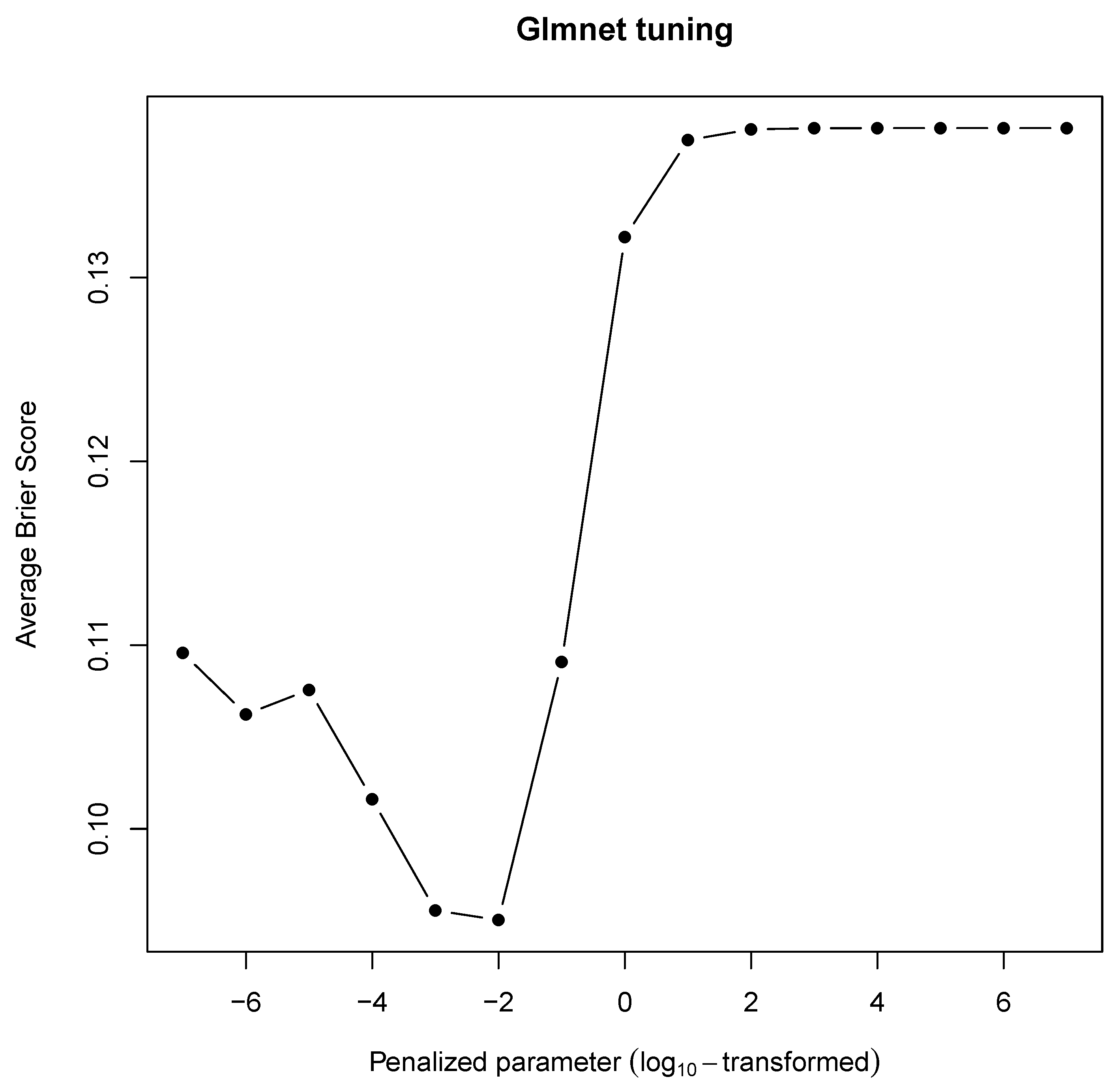
5.4.1. Logistic Regression

(1)
Introduction to Logistic Regression
Conventional logistic regression [20,21] can predict the occurrence probability of a specific outcome. The conditional probability of a positive outcome could be expressed with the formula below:
p ( x i ) = p ( Y = 1 | x i ) = 1 1 + e β 0 + β 1 x 1 + β 2 x 2 + + β d x d ,
where β i is the coefficient for the ith feature, and d is the total number of features. β 1 , β 2 , ⋯, β d can be solved by the elastic net approach [22,23,24] as follows:
m a x β 0 , β 1 n i = 1 n I ( y i = 1 ) l o g p ( x i ) + I ( y i = 0 ) l o g 1 p ( x i ) λ ( 1 α ) 1 2 β 2 2 + α β 1 ,
where
β 2 2 = β 1 2 + β 2 2 + + β d 2 a n d β 1 = β 1 + β 2 + + β d .
(2)
Logistic regression tuning
Glmnet [25] is an R language software package that can fit linear, logistic and multinomial, Poisson, and Cox regression models by maximizing the penalized likelihood. In order to predict the mutant score of each program statement in schedule.c, we use the ridge penalty algorithm in a glmnet software package to fit the logistic regression mode. Hence, during tuning hyper parameters, the penalized parameter α in the formula (14) is set to 0, and the penalized parameter λ is set to 10 i where i takes each integer from −7 to 7 in turn. In the cross-validation process, we use the Brier score as the model evaluation criterion. Under each penalized parameter, the five repeats of 5-fold cross-validation generate five Brier scores. We calculate the average of the five Brier scores under each candidate penalized parameter λ , so that we can use the average Brier score to represent the prediction effect of the model under the each candidate penalized parameter.
Figure 4 and Table 8 show the average Brier Score under each candidate value of the penalized parameter λ . In Figure 4, the profile shows a decrease in the average Brier score until the penalized value λ is 10 2 . Therefore, the numerically optimally value of the penalized parameter is 10 2 .

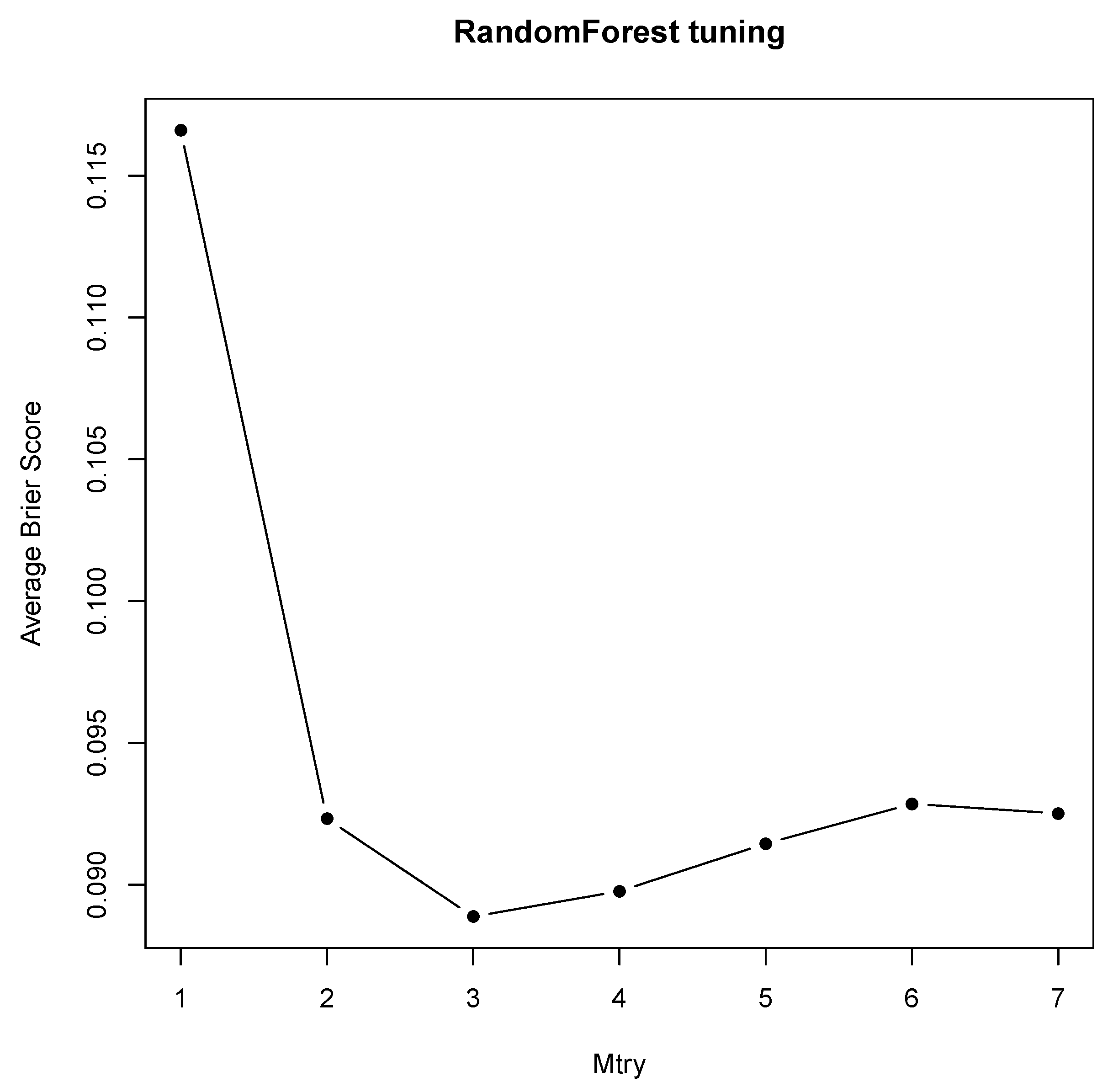
5.4.2. Random Forests

(1)
Introduction to Random Forest
The random forest model [26,27] can work for regression tasks and classification tasks generally. It is a tree-based model consisting of multiple decision trees. Each decision tree is created on an independent and random sample taken from the training data set.
The decision tree algorithm [18,28] is a top-down “greedy” approach that partitions the dataset into smaller subsets. This algorithm has a tree-like structure that predicts the value of a target variable based on several input variables. At each decision node, the features are split into two subsets and this process is repeated until the number of data in the splits falls below some threshold. According to the target variable’s type, decision trees can be divided into regression trees and classification trees. The purpose of classification tree is to classify, and its target variable takes discrete values. The purpose of regression trees is to build a regression model, its target variable takes continuous values.
For regression, the regression tree algorithm begins with the entire data set S and searches every distinct value of every independent variable to find the appropriate independent variable and split its value that partitions the data into two subsets ( S 1 and S 2 ) such that the overall sums of squares error
S S E = i S 1 ( y i y ¯ 1 ) 2 + i S 2 ( y i y ¯ 2 ) 2
are minimized, where y ¯ 1 and y ¯ 2 are the averages of the outcomes within subsets S 1 and S 2 , respectively. Then, within each of subsets S 1 and S 2 , this method searches again for the independent variable and splits its value that best reduces SSE. Because of the recursive splitting nature of regression trees, this method is also known as recursive partitioning.
For classification, the aim of classification trees is to partition the data into smaller, more homogeneous groups. Homogeneity in this context means that the nodes of the split are more pure. This purity is usually quantified by the entropy or Gini index. For the two-class problem, the Gini index for a given node is defined as
p 1 ( 1 p 1 ) + p 2 ( 1 p 2 ) ,
where p 1 and p 2 are the probabilities of Class 1 and Class 2, respectively.
In order to make a prediction for a given observation, the regression tree first analyzes which class this observation belongs to, and then takes the mean of the training data in the class as the prediction of this observation. When random forest algorithms are used, the result of regression question can be obtained by averaging predictions across all regression trees, and the result of the classification question can be obtained by a majority vote across all classification trees, respectively. The generalization error of a random forest depends on the errors of individual trees and the correlation between the trees.
(2)
Random forest tuning
The randomForest package [29] implements the random forest algorithm in the R environment. We use this software to predict statement mutation scores generated when the test suite executes on the program schedule.c. Because the statement mutation score can be considered as the probability of positive class in binary classification, we denote the positive class and negative class as 1 and 0, respectively, and let Random Forests run under regression mode to predict the probability of a positive class [30]. In order to obtain a good prediction model, the different hyper parameter combinations are tried. The most important hyper parameter is mtry, which is the number of independent variables randomly selected at each split. In our experiment, we tried multiple candidate values of mtry (from 1 to 7). The other important tuning parameter is ntree, which is the number of bootstrap samples in the random forest algorithm. In theory, the performance of a random forest model should be a monotonic function of the number of trees (ntree). However, when ntree is greater than a certain number, the performance of a random forest model can only improve slowly. In our experiment, ntree is set to 1000. Under each candidate value of the parameter mtry, we calculate the average of the five Brier scores generated from the five repeats of 5-fold cross-validation. Furthermore, we use these averages to express the prediction effects of the random forest model under different candidate values of hyperparameter mtry. Figure 5 and Table 9 show the average Brier score under each candidate value of the hyperparameter mtry. As shown in Figure 5, the average Brier scores show a U shape, whose minimum value occurs in m t r y = 3 . Therefore, 3 is the optimal value of mtry.

5.4.3. Artificial Neural Networks

(1)
Introduction to neural network
Neural networks [18,31] can be used not only for regression but also for classification. The outcome of a neural network is modeled by an intermediary set of unobserved variables called hidden units. The simplest neural network architecture is the single hidden layer feed-forward network.
The working process of the single hidden layer feed-forward neural network is as follows. During the entire work of the neural network, all input neurons representing the original independent variables x 1 , x 2 , ⋯, x s are first activated through the sensors perceiving the environment. Next, inside each hidden unit h k , all original independent variables are linearly combined to generate
u k ( x ) = β 0 k + j = 1 s β j k x j ,
where k = 1, 2,⋯, r and r is the number of the hidden units. Then, by a nonlinear function g k , u k ( x ) is typically transformed into the output of hidden unit h k as follows:
g k ( x ) = 1 1 + e u k ( x ) .
(i) When treating the neural network as a regression model, all g k ( x ) are linearly combined to form the output of neural network:
f ( x ) = γ 0 + k = 1 r γ k g k ( x ) .
All of the parameters β and γ can be solved by minimizing the the penalized sum of the squared residuals:
i = 1 n ( y i f ( x i ) ) 2 + λ k = 1 r j = 0 s β j k 2 + λ k = 0 r γ k 2 ,
where f ( x i ) and y i are the predicted result and the actual result related to the ith observed data, respectively.
(ii) Neural networks can also be used for classification. Unlike neural networks for regression, an additional nonlinear transformation is used on the linear combination of the outputs of hidden units.
When the neural network is used for binary classification, it uses
f * ( x ) = 1 1 + e f ( x ) = 1 1 + e ( γ 0 + k = 1 r γ k g k ( x ) )
to predict the class probability. The estimation of the parameters γ and β can be solved by minimizing the penalized cross-entropy
i = 1 n y i log f ( x i ) + ( 1 y i ) log ( 1 f ( x i ) ) + λ k = 1 r j = 0 s β j k 2 + λ k = 0 r γ k 2 ,
where y i is the 0 / 1 indicator for the positive class. The neural network algorithm can also be used for multi-class classification. In this situation, the softmax transform outputs the probability that the sample x belongs to the lth class. Except the single hidden layer feed-forward network, there are many other types of models. For example, the famous deep learning approaches consist of multiple hidden layers.
(2)
Neural network tuning
As we said before, the our model must not be too complicated, so we select R package nnet [32] to predict the statement mutation scores of the test suite on schedule.c. The software package nnet implements a feed-forward neural network with a single hidden layer. The λ and r in formula (22) represent the weight decay and the number of units in the hidden layer, respectively. They are denoted as d e c a y and s i z e in nnet package, respectively. Therefore, d e c a y is the regularization parameter to avoid over-fitting.
In our experiment, s i z e is set in turn to each integer value between one and then. At the same time, the d e c a y was set to 10 i where i takes each integer value from −4 to 5 in turn.
Figure 6 and Table 10 show the average Brier scores under the each candidate combinations of s i z e and d e c a y . From them, we can know that the optimal combination of the weight decay and hidden unit number is d e c a y = 10 2 and s i z e = 8 because, at this time, the minimum average Brier score appears.

5.4.4. Support Vector Machines

(1)
Introduction to support vector machine
Given a set of n training instances x 1 , x 2 , , x n , the goal of support vector machine is to find a hyperplane that separates the positive and the negative training instances with the maximum margin and minimum misclassification error. The training of support vector machine is equivalent to solving the following optimization problem:
min w , b , ζ i 1 2 w 2 + C i = 1 n ζ i s u b j e c t t o y i ( w T x i + b ) 1 ζ i ζ i 0 , i = 1 , 2 , , n ,
where w is the normal vector of the maximum-margin hyperplane w T x + b = 0 , C is the regularization parameter, ζ i indicates a non-negative slack variable to tolerant some training data falling in the wrong side of the hyperplane, and b is a bias. The parameter C specifies the cost of a violation to the margin. When C is small, the margins will be wide and many support vectors will be on the margin or will violate the margin. When C is large, the margins will be narrow and there will be few support vectors on the margin or violating the margin.
The maximum-margin hyperplane can be obtained by solving the above problem. Given new data x , f ( x ) = w T x + b represents the signed distance between x and the hyperplane. We can classify the new data x based on the sign of f ( x ) .
If the original problem is stated in a finite-dimensional space, it often happens that the sets to discriminate are not linearly separable. For solving this problem, a support vector machine maps the original finite-dimensional space into a higher-dimensional space, making the separation easier. Let ϕ ( x ) denote the vector after x mapping. In this higher-dimensional space, the optimization problem can be rewritten into
min w , b , ζ i 1 2 w 2 + C i = 1 n ζ i
s u b j e c t t o y i ( w T ϕ ( x i ) + b ) 1 ζ i
ζ i 0 , i = 1 , 2 , , n
or expressed in the dual form
min α i = 1 n α i + 1 2 i = 1 n j = 1 n α i α j y i y j k ( x i , x j )
s u b j e c t t o i = 1 n α i y i = 0
0 α i C , i = 1 , 2 , , n ,
where k ( x i , x j ) = ϕ ( x i ) T ϕ ( x j ) defines the kernel function greatly reducing the computational cost.
By solving the above optimization problem, the optimal α i * and b * can be obtained. Therefore, the maximum-margin hyperplane in the higher-dimensional space is
w * T ϕ ( x ) + b = i = 1 n α i * y i ϕ ( x i ) T ϕ ( x ) + b * = i = 1 n α i * y i k ( x i , x ) + b * .
The kernel trick allows the support vector machine model to produce extremely flexible decision boundaries. The most common kernel functions are listed in Table 11:
The original SVM can be used for classification and regression without probability information. To solve this problem, Platt [33] proposed to use a logistic function to convert the decision value from a binary support vector machine to a probability. Formally, the probability of data x i being a positive instance is defined as follows:
P ( y i = 1 | x i ) = 1 1 + e x p ( A f ( x i ) + B ) ,
where f ( x ) = w T ϕ ( x ) + b is the maximum-margin hyperplane. The parameters A and B are derived by minimizing the negative log-likelihood of the training data:
i = 1 n [ t i l o g ( P ( y i = 1 | x i ) ) + ( 1 t i ) l o g ( 1 P ( y i = 1 | x i ) ) ]
where
t i = n + + 1 n + + 2 i f y i = 1 , 1 n + 2 i f y i = 1 .
n + denotes the number of positive training instances (i.e., y i = 1), and n denotes the number of negative training instances (i.e., y i = −1). Newton’s method with backtracking is a commonly used approach to solve the above optimization problem [34] and is implemented in LibSVM. Besides the binary classification, the support vector machine can also compute the class probabilities for the multi-class problem using one-against-one (i.e., pairwise) approach [35].
(2)
Support vector machine tuning
Support vector machine algorithms are provided in the software package kernlab [36] written in the R language. We built the support vector machine based on the radial basis kernel function provided by this package. A radial basis kernel function maps the independent variables to an infinite-dimensional space. The regularization parameter C in formula (23) is called cost parameter in kernlab. A smaller C results in a smoother decision surface and a larger C results in a flexible model that strives to classify all training data correctly. The radial basis kernel function in kernlab package is shown in Table 11, where the parameter σ represents the inverse kernel width. A larger σ means a narrower radial basis kernel function.
When we use kernlab to predict the statement mutation scores of schedule.c, we hope to get the Brier score as small as possible by tuning C and σ . For this purpose, we first set the parameter σ to the median of x x 2 [18,37,38]. Next, let the parameter C take respectively as 2 5 , 2 3 , 2 1 , 2 1 , 2 3 , 2 5 , 2 7 , 2 9 , 2 11 , 2 13 and 2 15 . Then, under each candidate value of C, we use the five repeats of 5-fold cross-validation to calculate the average Brier scores.
Figure 7 and Table 12 show the average Brier score generated by five repeats of 5-fold cross-validation at each candidate value of C. As shown in Figure 7, although there was a relatively large fluctuation, the average Brier score shows a general trend of first decreasing and then rising. From this figure, we can know that C = 2 1 is the optimally value of the regularization parameter. At this time, the average Brier score reaches a minimum 0.0933.

5.4.5. Symbolic Regression

(1)
Introduction to symbolic regression
Symbolic regression can also be called function modeling. Based on the given data, it can automatically find the functional relationship, such as 2 x 3 + 5 , cos ( x ) + 1 / e y , etc., between independent variables and dependent variables.
Throughout the modeling process, a function model f ( x ) is always coded as a symbolic expression tree. The input of symbolic regression is a data set, and the genetic programming method is often used to determine f ( x ) . The genetic programming constantly changes an old function model into a new better fitted one by selecting the function with the better fitness value. A possible and frequently used fitness function is the average squared difference between the values predicated by f ( x ) and the actually observed values y as follows:
M S E ( f ( x ) , y ) = 1 n i = 1 n ( f ( x i ) y i ) 2 .
Mutation operations and crossover operations are the two important ways to change function model f ( x ) . A mutation operation directly changes a symbolic expression sub tree, and a crossover operation cuts a symbolic expression sub tree and replace it with a sub tree in another symbolic expression tree.
(2)
Symbolic regression tunning
The symbolic regression tool rgp [39] is an implementation of genetic programming methods in the R environment. We use rgp to predict the statement mutation scores of schedule.c. In our symbolic regression experiment, the most basic mathematical operators are set to the operators +, −, *, /, sin. An important tuning parameter in rgp is p o p u l a t i o n S i z e , which means the number of individuals included in a population, and is set to 100 in our experiment.
Another important tuning parameter is the number of evolution generations. Too few evolutionary generations produce an under-fitting, whereas too many evolutionary generations produce an over-fitting. We did a grid search to determine the optimal number of the generations, which minimizes the average Brier score. Because we need to complete the model fitting in a relatively short time, the number of evolution generations cannot be set too large. In our experiment, the candidate number of evolution generations is set to 3, 6, 9, 12, 15, 18, respectively. The five repeats of five-fold cross-validation are used to calculate the evolution effects (i.e., the average Brier scores) under each candidate number of evolution generations.
As shown in Table 13 and Figure 8, the average Brier scores oscillated down. In the 12th generation evolution, the smallest average Brier score 0.1504 appeared.

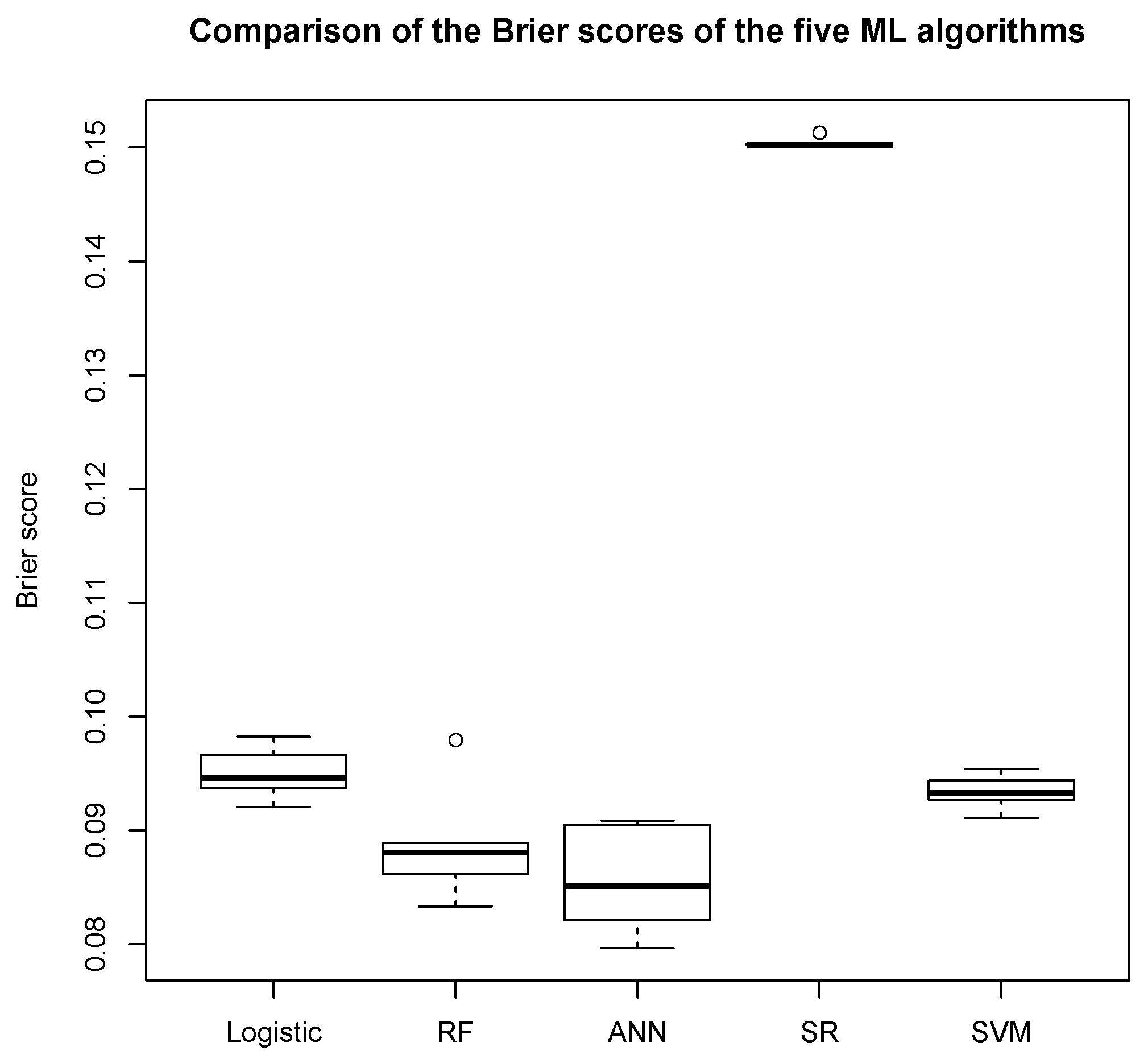
5.4.6. Comparing Models

Once the hyper parameters in the above five models have been determined for the above five models, we face the question: how do we choose among multiple models? The logistic regression model is used to set the baseline performance because its mathematical expression is simple and operation speed is fast. If other predictive models do not surpass it, the logistic regression model is used in future actual forecasting.
The boxplot in Figure 9 shows, under the condition that the Brier score is the standard, the neural network does the best job about predicting the statement mutation scores. The second best is the random forest model, which is a little better than the support vector machine model. The logistic model is second to last and greatly exceeded the symbolic regression.

5.4.7. Testing Predictions in Practice

According to Figure 9 and Table 8, Table 9 and Table 10, Table 12 and Table 13, we know that, in the process of repeated cross-validation, the average Brier scores of the logistic regression, random forest, neural network, support vector machine and symbolic regression are 0.0950, 0.0888, 0.0856, 0.0933 and 0.1504, respectively. Therefore, the neural network is the best model because its average Brier score is lower than other models. To further demonstrate the predictive effect of the neural network model on the schedule.c, we did the two following things. Firstly, we apply the neural network model, whose hyper-parameters have been tuned according to the method in Section 5.4.3, to predict the statement mutation scores of schedule.c. Under the condition that the schedule.c is used as the experiment subject, we calculate the mean absolute error between all statement mutation scores obtained by the neural network prediction and all real statement mutation scores. The experiment result shows the mean absolute error reaches 0.1205. Secondly, we randomly select 34 statements in schedule.c, and their two kinds of statement mutation scores are shown in Figure 10. In this figure, the horizontal coordinate represents the real statement mutation score, and the vertical coordinate represents the statement mutation score predicted by the neural network model. Each circle represents a statement, and the distance between each short dashed line and diagonal line is 0.1. From this figure, we can see that more than 60% of the statements are located between the two short dashed lines.

5.5. Further Confirmation of the Optimization Model

To further confirm that the prediction effect of the neural network is the best, we compared the five machine learning models again under the condition that the program tcas.c is used as the experimental subject. In the process of repeated cross-validation, the average Brier score of the neural network model reaches 0.1164. The average Brier scores of the logistic regression, the support vector machine, the random forest and the symbolic regression are 0.1233, 0.1249, 0.1289 and 0.1373, respectively. Therefore, the neural network is once again considered the best model because its average Brier score is lower than other models. To further demonstrate the predictive effect of the neural network model on the tcas.c, we apply the neural network model, whose hyper-parameters have been tuned according to the method in Section 5.4.3, to predict the statement mutation scores of tcas.c. Under the condition that the tcas.c is used as the experiment subject, the mean absolute error between real statement mutation scores and the statement mutation scores predicted by the tuned neural network reaches 0.1198. In order to illustrate the prediction results of the neural network more vividly, we randomly selected 31 statements in the program tcas.c. Their real statement mutation scores and the corresponding predicted mutation scores are shown in Figure 11.
Through the above analysis, we can see that, whether the experiment subject is schedule.c or tcas.c, the average Brier scores of the neural network are both the minimums. Thus, we recommend the single hidden layer feedforward neural network as the best model. In the two experiments, the mean absolute error between the statement mutation scores predicted by the neural network model and the real statement mutation scores both approximately reach 0.12.

6. Structure of the Automated Prediction Tool

The work process of our automatic analysis tool consists of the five parts, as shown in Figure 12: extracting the features of the statements in the program under testing, generating mutants, executing test suite on the each mutants, establishing the neural network model, and predicting the statement mutation scores.
In the first part, we extract the features of statements in the program under testing. First, we execute each test case and construct its execution impact graph with the open source software giri [40]. Giri was originally a dynamic program slice tool and is currently modified by us. Next, we traverse the statement instances in reverse order of the execution history of the test cases. Whenever we visit a statement instance, we compute its features. After calculating the features of each statement instance, we calculate the features of each program statement according to the corresponding the statement instances.
In the second part, we generate mutants. We first build a mutation operator set. In our experiments, the mutation operator set consists of the 22 mutation operators, which exist in the open source mutant generate tool ProteumIM2.0 [12]. These operators include u-Cccr, u-OEAA, u-OEBA, u-OESA, u-CRCR, u-Ccsr, u-OAAN, u-OABN, u-OALN, u-OARN, u-OASN, u-OCNG, u-OLAN, u-OLBN, u-OLLN, u-OLNG, u-OLRG, u-OLSN, u-ORBN, u-ORLN, u-ORRN and u-ORSN. Next, we use these mutation operators to randomly construct 200 mutants, each of which is the program with a software bug.
In the third part, we execute the test suite on each mutant and record the corresponding identification result.
In the fourth part, we take the features of the mutant as independent variables and the identification result of the mutant as dependent variables to construct the prediction model with the neural network.
In the fifth part, we predict the mutation scores of each program statement with the constructed model.

7. Conclusions

In this paper, we predicted statement mutation scores while using a single hidden layer feedforward neural network and seven statement features. As analyzed in Section 5, each experimental result shows that the neural network is the best prediction model from the standpoint of the mean absolute error. The experimental results on two c programs demonstrate that our method can directly predict statement mutant scores approximately. The experiment results also show that the seven statement features that represent the dynamic program execution and testing process can basically reflect the impact of statements on program output.
However, two shortcomings need to be improved. Firstly, a part of statement features weakly related to program outputs still need to be discovered. If the real mutation score of a statement is low, then this statement usually only has some statement features weakly related to program outputs. In this case, the prediction effect of my model is not good because we only found a part of weakly relevant statement features, and the other part of the weakly correlated sentence features still need to be discovered.
Secondly, in this paper, we assume the controlling expression has no side effect. However, in a few cases, a controlling expression has a side effect. In this case, the execution instance of the controlling expression may have some impact successors. For example, if there is a controlling expression if(x > y++) in the original program, then the execution result of y++ will be changed when it is executed a test case, so that it impacts subsequent statement instances containing y variables. In this situation, the methods mentioned in Section 3.1.4, Section 3.2.4, Section 3.3.2, Section 3.4.2 and Section 3.5.3 are no longer applicable, and the corresponding algorithm needs to be redesigned.
In the future, we also plan to predict the statement mutation scores with the prediction model established by other programs. In this case, the users can train a prediction model with the data records from other programs beforehand. Using this pre-trained model, users can directly predict the statement mutation scores of the current program.

Author Contributions

Conceptualization, L.T.; methodology, L.T.; Supervision, Y.W. and Y.G.; writing—original draft preparation, L.T.

Funding

This work was supported by the National Natural Science Foundation of China (No. U1736110), the National Natural Science Foundation of China (No. 61702044), and the Fundamental Research Funds for the Central Universities (No. 2017RC27).

Conflicts of Interest

The authors declare no conflicts of interest.

Abbreviations

The following abbreviations are used in this manuscript:
V g value impact set of the statement s g
x v i ( s g ) value impact factor of the statement s g
V g , t k h value impact set of the statement instance s g , t k h
V r , z , t k l value impact set of the branch instance B r , z , t k l
P g path impact set of the statement s g
x p i ( s g ) path impact factor of the statement s g
P g , t k h path impact set of the statement instance s g , t k h
P r , z , t k l path impact set of the branch instance B r , z , t k l
V g generalized value impact set of the statement s g
x g v i ( s g ) generalized value impact factor of the statement s g
V g , t k h generalized value impact set of the statement instance s g , t k h
P g generalized path impact set of the statement s g
x g p i ( s g ) generalized path impact factor of the statement s g
P g , t k h path impact set of the generalized statement instance s g , t k h
L g latent impact set of statement s g
x l i ( s g ) latent impact factor of statement s g
L g , t k h latent impact set of statement instance s g , t k h
x i h ( s g ) information hidden factor of statement s g

References

  1. Andrews, J.H.; Briand, L.C.; Labiche, Y. Is mutation an appropriate tool for testing experiments? In Proceedings of the 27th International Conference on Software Engineering, St. Louis, MO, USA, 15–21 May 2005; pp. 402–411. [Google Scholar]
  2. DeMillo, R.A.; Lipton, R.J.; Sayward, F.G. Hints on test data selection: Help for the practicing programmer. Computer 1978, 11, 34–41. [Google Scholar] [CrossRef]
  3. Mirshokraie, S.; Mesbah, A.; Pattabiraman, K. Efficient JavaScript mutation testing. In Proceedings of the 2013 IEEE Sixth International Conference on Software Testing, Verification and Validation, Luxembourg, 18–22 March 2013; pp. 74–83. [Google Scholar]
  4. Jia, Y.; Harman, M. An analysis and survey of the development of mutation testing. IEEE Trans. Softw. Eng. 2011, 37, 649–678. [Google Scholar] [CrossRef]
  5. Frankl, P.G.; Weiss, S.N.; Hu, C. All-uses vs mutation testing: An experimental comparison of effectiveness. J. Syst. Softw. 1997, 38, 235–253. [Google Scholar] [CrossRef]
  6. Maldonado, J.C.; Delamaro, M.E.; Fabbri, S.C.; da Silva Simão, A.; Sugeta, T.; Vincenzi, A.M.R.; Masiero, P.C. Proteum: A family of tools to support specification and program testing based on mutation. In Mutation Testing for the New Century; Springer: Berlin/Heidelberg, Germany, 2001; pp. 113–116. [Google Scholar]
  7. Acree, A.T., Jr. On Mutation; Technical Report; Georgia Inst of Tech Atlanta School of Information and Computer Science: Atlanta, GA, USA, 1980. [Google Scholar]
  8. Zhang, L.; Hou, S.S.; Hu, J.J.; Xie, T.; Mei, H. Is operator-based mutant selection superior to random mutant selection? In Proceedings of the 32nd ACM/IEEE International Conference on Software Engineering, Cape Town, South Africa, 1–8 May 2010; Volume 1, pp. 435–444. [Google Scholar]
  9. Hussain, S. Mutation Clustering. Master’s Thesis, Kings College London, London, UK, 2008. [Google Scholar]
  10. Gligoric, M.; Zhang, L.; Pereira, C.; Pokam, G. Selective mutation testing for concurrent code. In Proceedings of the 2013 International Symposium on Software Testing and Analysis, Lugano, Switzerland, 15–20 July 2013; pp. 224–234. [Google Scholar]
  11. Offutt, A.J.; Rothermel, G.; Zapf, C. An experimental evaluation of selective mutation. In Proceedings of the 1993 15th International Conference on Software Engineering, Baltimore, MD, USA, 17–21 May 1993; pp. 100–107. [Google Scholar]
  12. Zhang, J.; Zhang, L.; Harman, M.; Hao, D.; Jia, Y.; Zhang, L. Predictive mutation testing. IEEE Trans. Softw. Eng. 2018. [Google Scholar] [CrossRef]
  13. Jalbert, K.; Bradbury, J.S. Predicting mutation score using source code and test suite metrics. In Proceedings of the First, International Workshop on Realizing AI Synergies in Software Engineering, Zurich, Switzerland, 5 June 2012; pp. 42–46. [Google Scholar]
  14. Goradia, T. Dynamic impact analysis: A cost-effective technique to enforce error-propagation. In Proceedings of the 1993 ACM SIGSOFT International Symposium on Software Testing and Analysis, Cambridge, MA, USA, 28–30 June 1993; Volume 18, pp. 171–181. [Google Scholar]
  15. C programming Language Standard—C99. Available online: https://en.wikipedia.org/wiki/C99 (accessed on 19 August 2019).
  16. The Program schedule.c. Available online: https://www.thecrazyprogrammer.com/2014/11/c-cpp-program-forpriority-scheduling-algorithm.html (accessed on 19 August 2019).
  17. The Program tcas.c. Available online: https://sir.csc.ncsu.edu/php/showfiles.php (accessed on 19 August 2019).
  18. Kuhn, M.; Johnson, K. Applied Predictive Modeling; Springer: Berlin/Heidelberg, Germany, 2013; Volume 26. [Google Scholar]
  19. Brier, G.W. Verification of forecasts expressed in terms of probability. Mon. Weather Rev. 1950, 78, 1–3. [Google Scholar] [CrossRef]
  20. Hosmer, D.W., Jr.; Lemeshow, S.; Sturdivant, R.X. Applied Logistic Regression; John Wiley & Sons: Hoboken, NJ, USA, 2013; Volume 398. [Google Scholar]
  21. Harrell, F.E. Regression Modeling Strategies; Springer: Berlin/Heidelberg, Germany, 2001. [Google Scholar]
  22. Hastie, T.; Tibshirani, R.; Wainwright, M. Statistical Learning with Sparsity: The Lasso and Generalizations; Chapman and Hall/CRC: Boca Raton, FL, USA, 2015. [Google Scholar]
  23. Friedman, J.; Hastie, T.; Tibshirani, R. Regularization paths for generalized linear models via coordinate descent. J. Stat. Softw. 2010, 33, 1. [Google Scholar] [CrossRef] [PubMed]
  24. Tibshirani, R. Regression Shrinkage and Selection Via the Lasso. J. R. Stat. Soc. Ser. B 1994, 58, 267–288. [Google Scholar] [CrossRef]
  25. Glmnet. Available online: https://CRAN.R-project.org/package=glmnet (accessed on 19 August 2019).
  26. Breiman, L. Some Infinity Theory for Predictor Ensembles; Technical Report 579; Statistics Dept. UCB: Berkeley, CA, USA, 2000. [Google Scholar]
  27. Breiman, L. Consistency for a Simple Model of Random Forests; Technical Report (670); University of California at Berkeley: Berkeley, CA, USA, 2004. [Google Scholar]
  28. Quinlan, J.R. Simplifying decision trees. Int. J. Hum.-Comput. Stud. 1999, 51, 497–510. [Google Scholar] [CrossRef] [Green Version]
  29. The randomForest. Available online: https://cran.r-project.org/web/packages/randomForest/index.html (accessed on 19 August 2019).
  30. Li, C. Probability Estimation in Random Forests. Master’s Thesis, Department of Mathematics and Statistics, Utah State University, Logan, UT, USA, 2013. [Google Scholar]
  31. Demuth, H.B.; Beale, M.H.; De Jess, O.; Hagan, M.T. Neural Network Design, 2nd ed.; Martin Hagan: Stillwater, OK, USA, 2014. [Google Scholar]
  32. R Package nnet. Available online: https://CRAN.R-project.org/package=nnet (accessed on 19 August 2019).
  33. Platt, J.C. Probabilistic Outputs for Support Vector Machines and Comparisons to Regularized Likelihood Methods. In Advances in Large Margin Classifiers; MIT Press: Cambridge, MA, USA, 1999; pp. 61–74. [Google Scholar]
  34. Lin, H.T.; Lin, C.J.; Weng, R.C. A note on Platt’s probabilistic outputs for support vector machines. Mach. Learn. 2007, 68, 267–276. [Google Scholar] [CrossRef]
  35. Hsu, C.W.; Lin, C.J. A comparison of methods for multiclass support vector machines. IEEE Trans. Neural Netw. 2002, 13, 415–425. [Google Scholar] [PubMed]
  36. Software Package Kernlab. Available online: https://CRAN.R-project.org/package=kernlab (accessed on 19 August 2019).
  37. Caputo, B.; Sim, K.; Furesjo, F.; Smola, A. Appearance-based object recognition using SVMs: Which kernel should I use? In Proceedings of the NIPS Workshop on Statistical Methods for Computational Experiments in Visual Processing and Computer Vision, Whistler, BC, Canada, 12–14 December 2002; Volume 2002. [Google Scholar]
  38. Karatzoglou, A.; Smola, A.; Hornik, K.; Zeileis, A. kernlab—An S4 package for kernel methods in R. J. Stat. Softw. 2004, 11, 1–20. [Google Scholar] [CrossRef]
  39. The Symbolic Regression Tool Rgp. Available online: http://www.rdocumentation.org/packages/rg (accessed on 19 August 2019).
  40. Sahoo, S.K.; Criswell, J.; Geigle, C.; Adve, V. Using likely invariants for automated software fault localization. In Proceedings of the 18th International Conference on Architectural Support for Programming Languages and Operating Systems, ASPLOS 2013, Houston, TX, USA, 16—20 March 2013; ACM SIGARCH Computer Architecture News. Volume 41, pp. 139–152. [Google Scholar]
Figure 1. The execution impact graph G 1 formed when Program 1 is executed by test case 1.
Mathematics 07 00778 g001
Figure 2. The execution impact graph G 2 formed when Program 1 is executed by test case 2.
Mathematics 07 00778 g002
Figure 3. The execution impact graph G 3 formed when Program 1 is executed by test case 3.
Mathematics 07 00778 g003
Figure 4. The performance profile of the logistic regression for predicting the statement mutation scores.
Mathematics 07 00778 g004
Figure 5. The performance profile of the random forest for predicting the statement mutation scores.
Mathematics 07 00778 g005
Figure 6. The performance profile of the neural network for predicting the statement mutation scores.
Mathematics 07 00778 g006
Figure 7. The performance profile of the support vector for predicting the statement mutation scores.
Mathematics 07 00778 g007
Figure 8. Rgp tuning.
Mathematics 07 00778 g008
Figure 9. Comparison of the Brier scores of the five machine learning models for schedule.c.
Mathematics 07 00778 g009
Figure 10. Comparing the real statement mutation scores and the predicted statement mutation scores in schedule.c by the artificial neural network.
Mathematics 07 00778 g010
Figure 11. Comparing the real statement mutation scores and the predicted statement mutation scores in tcas.c by the artificial neural network.
Mathematics 07 00778 g011
Figure 12. The structure of Automated Analysis Tool.
Mathematics 07 00778 g012
Table 1. Main differences among mutation reduction methods.
MethodKey TechnologyTime CostTarget
random mutationsimple random samplinglowestimating program mutation score
mutant clusteringstratified samplinglowestimating program mutation score
selective mutationnon-probability samplinghighestimating program mutation score
predictive mutationsupervised learninglowestimating program mutation score
classifying mutants
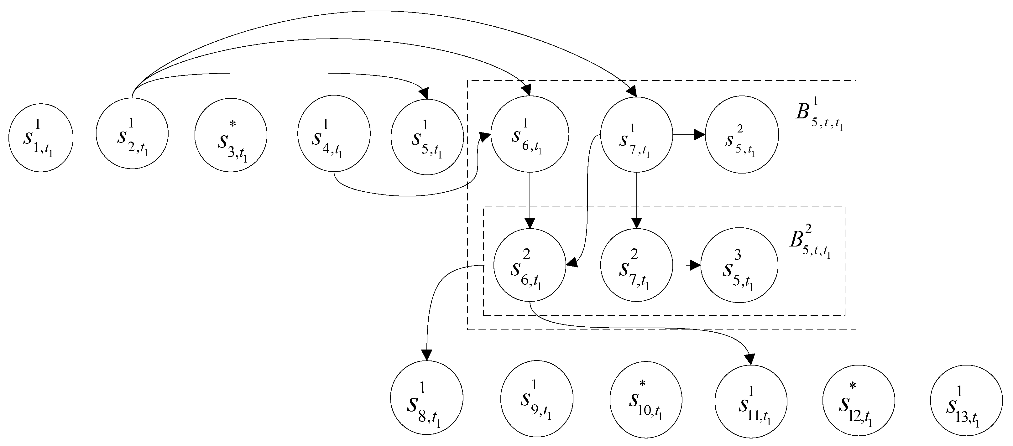
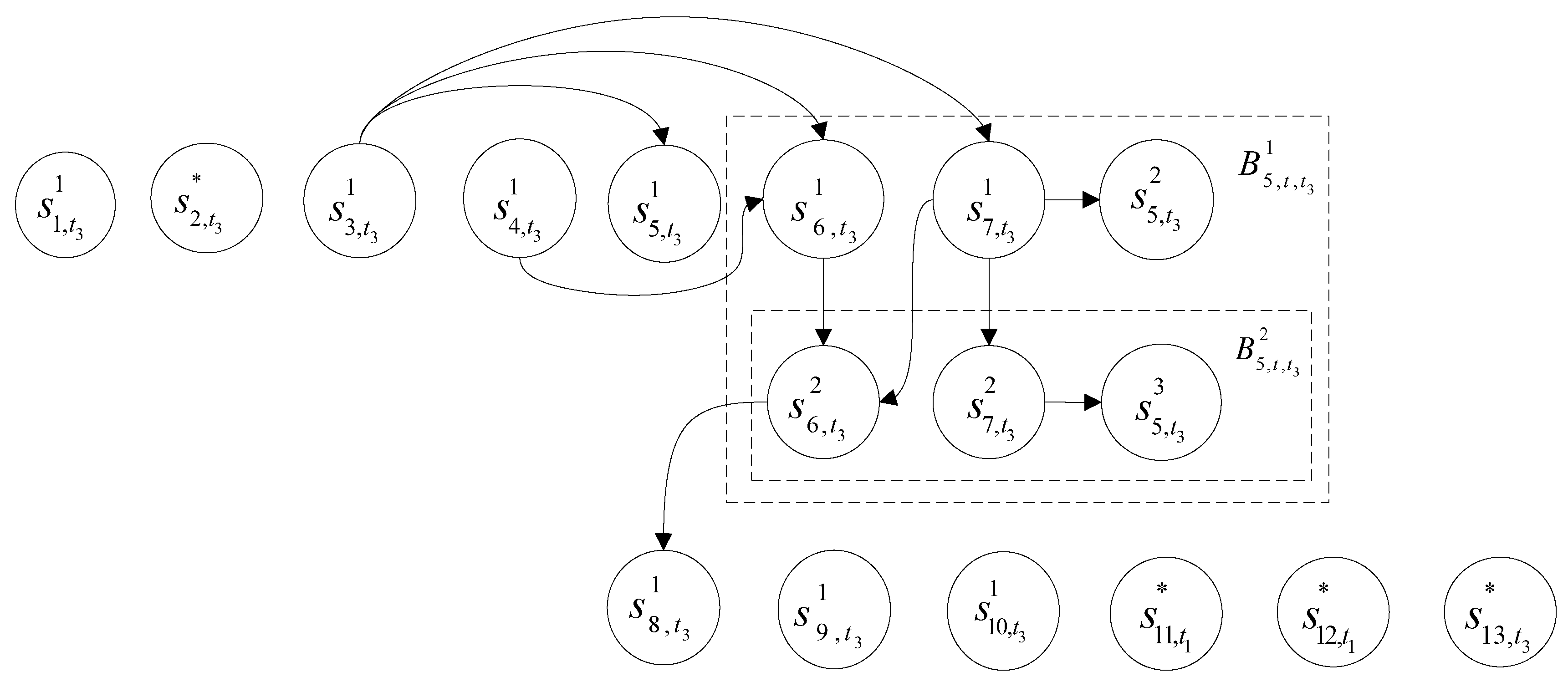
Table 2. The execution history of the test cases.
Test CaseProgram OutputExecution HistoryBranch Instances in Loop
m = 4, n = 1fac = 6, class 1 ( s 13 ) H 1 : s 1 , t 1 1 , s 2 , t 1 1 , s 4 , t 1 1 , s 5 , t 1 1 , s 6 , t 1 1 , s 7 , t 1 1 , s 5 , t 1 2 s 6 , t 1 2 , s 7 , t 1 2 , s 5 , t 1 3 , s 8 , t 1 1 , s 9 , t 1 1 , s 11 , t 1 1 , s 13 , t 1 1 B 5 , t , t 1 1 = { s 6 , t 1 1 , s 7 , t 1 1 , s 5 , t 1 2 , s 6 , t 1 2 , s 7 , t 1 2 ,
s 5 , t 1 3 }, B 5 , t , t 1 2 = { s 6 , t 1 2 , s 7 , t 1 2 , s 5 , t 1 3 }
m = 2, n = 2fac = 1, class 2 ( s 12 ) H 2 : s 1 , t 2 1 , s 3 , t 2 1 , s 4 , t 2 1 , s 5 , t 2 1 , s 8 , t 2 1 , s 9 , t 2 1 , s 11 , t 2 1 , s 12 , t 2 1
m = 1, n = 4fac = 6, class 1 ( s 10 ) H 3 : s 1 , t 3 1 , s 3 , t 3 1 , s 4 , t 3 1 , s 5 , t 3 1 , s 6 , t 3 1 , s 7 , t 3 1 , s 5 , t 3 2 s 6 , t 3 2 , s 7 , t 3 2 , s 5 , t 3 3 , s 8 , t 3 1 , s 9 , t 3 1 , s 10 , t 3 1 B 5 , t , t 1 1 = { s 6 , t 1 1 , s 7 , t 3 1 , s 5 , t 3 2 , s 6 , t 3 2 , s 7 , t 3 2 ,
s 5 , t 3 3 }, B 5 , t , t 3 2 = { s 6 , t 3 2 , s 7 , t 3 2 , s 5 , t 3 3 }
Table 3. The first five impact sets of all statement instances in Program 1.
Statement
Instance
Direct Impact
Successors
Value
Impact Set
Path
Impact Set
Generalized
Value Impact Set
Generalized
Path Impact Set
Latent
Impact Set
s 13 , t 1 1 s 13 , t 1 1
s 11 , t 1 1 s 11 , t 1 1 s 13 , t 1 1 B 11 , t , t 1 1
s 9 , t 1 1 s 9 , t 1 1 s 13 , t 1 1 B 9 , t , t 1 1
s 8 , t 1 1 s 8 , t 1 1
s 5 , t 1 3 s 5 , t 1 3 B 5 , t , t 1 3
s 7 , t 1 2 s 5 , t 1 3 s 5 , t 1 3 B 5 , t , t 1 3
s 6 , t 1 2 s 8 , t 1 1 , s 11 , t 1 1 s 8 , t 1 1 s 11 , t 1 1 s 13 , t 1 1 B 11 , t , t 1 1
s 5 , t 1 2 s 5 , t 1 2 s 8 , t 1 1 s 11 , t 1 1
s 7 , t 1 1 s 5 , t 1 2 , s 6 , t 1 2 , s 7 , t 1 2 s 8 , t 1 1 s 5 , t 1 2 , s 5 , t 1 3 , s 11 , t 1 1 s 8 , t 1 1 , s 13 , t 1 1 s 11 , t 1 1 B 5 , t , t 1 3 , B 11 , t , t 1 1
s 6 , t 1 1 s 6 , t 1 2 s 8 , t 1 1 s 11 , t 1 1 s 13 , t 1 1 B 11 , t , t 1 1
s 5 , t 1 1 s 5 , t 1 1 s 8 , t 1 1 s 11 , t 1 1
s 4 , t 1 1 s 6 , t 1 1 s 8 , t 1 1 s 11 , t 1 1 s 13 , t 1 1 B 11 , t , t 1 1
s 2 , t 1 1 s 5 , t 1 1 , s 6 , t 1 1 , s 7 , t 1 1 s 8 , t 1 1 s 5 , t 1 1 , s 5 , t 1 2 , s 5 , t 1 3 , s 11 , t 1 1 s 8 , t 1 1 , s 13 , t 1 1 s 11 , t 1 1 B 5 , t , t 1 3 , B 11 , t , t 1 1
s 1 , t 1 1 s 1 , t 1 1 s 8 , t 1 1 s 5 , t 1 1 , s 5 , t 1 2 , s 5 , t 1 3 , s 11 , t 1 1 B 1 , f , t 1 1
s 12 , t 2 1 , s 12 , t 2 1
s 11 , t 2 1 , s 11 , t 2 1 s 12 , t 2 1 B 11 , f , t 2 1
s 9 , t 2 1 s 9 , t 2 1 s 12 , t 2 1 B 9 , t , t 2 1
s 8 , t 2 1 s 8 , t 2 1
s 5 , t 2 1 s 5 , t 2 1 B 5 , t , t 2 1
s 4 , t 2 1 s 8 , t 2 1 , s 11 , t 2 1 s 8 , t 2 1 s 11 , t 2 1 s 12 , t 2 1 B 11 , f , t 2 1
s 3 , t 2 1 s 5 , t 2 1 s 5 , t 2 1 B 5 , t , t 2 1
s 1 , t 2 1 s 1 , t 2 1 s 5 , t 2 1 B 5 , t , t 2 1
s 10 , t 3 1 s 10 , t 3 1
s 9 , t 3 1 s 9 , t 3 1 s 10 , t 3 1 B 9 , f , t 3 1
s 8 , t 3 1 s 8 , t 3 1
s 5 , t 3 3 s 5 , t 3 3 B 5 , t , t 3 3
s 7 , t 3 2 s 5 , t 3 3 s 5 , t 3 3 B 5 , t , t 3 3
s 6 , t 3 2 s 8 , t 3 1 s 8 , t 3 1
s 5 , t 3 2 s 5 , t 3 2 s 8 , t 3 1
s 7 , t 3 1 s 5 , t 3 2 , s 6 , t 3 2 , s 7 , t 3 2 s 8 , t 3 1 s 5 , t 3 2 , s 5 , t 3 2 s 8 , t 3 1 B 5 , t , t 3 3
s 6 , t 3 1 s 6 , t 3 2 s 8 , t 3 1
s 5 , t 3 1 s 5 , t 3 1 s 8 , t 3 1
s 4 , t 3 1 s 6 , t 3 1 s 8 , t 3 1
s 3 , t 3 1 s 5 , t 3 1 , s 6 , t 3 1 , s 7 , t 3 1 s 8 , t 3 1 s 5 , t 3 1 , s 5 , t 3 2 , s 5 , t 3 3 s 8 , t 3 1 B 5 , t , t 3 3
s 1 , t 3 1 s 1 , t 3 1 s 8 , t 3 1 s 5 , t 3 1 , s 5 , t 3 2 , s 5 , t 3 3 B 1 , t , t 3 1
Table 4. The first five impact sets of all statements in Program 1.
Statement
instance
Value
Impact Set
Path
Impact Set
Generalized
Value Impact Set
Generalized
Path Impact Set
Latent
Impact Set
s 1 s 1 , t 1 1 , s 1 , t 2 1 , s 1 , t 3 1 s 8 , t 1 1 , s 8 , t 3 1 s 5 , t 1 1 , s 5 , t 1 2 , s 5 , t 1 3 , s 11 , t 1 1
, s 5 , t 2 1 , s 5 , t 3 1 , s 5 , t 3 2 , s 5 , t 3 3
B 1 , f , t 1 1 , B 5 , t , t 2 1 , B 1 , t , t 3 1
s 2 s 8 , t 1 1 s 5 , t 1 1 , s 5 , t 1 2 , s 5 , t 1 3 , s 11 , t 1 1 s 8 , t 1 1 , s 13 , t 1 1 s 11 , t 1 1 B 5 , t , t 1 3 , B 11 , t , t 1 1
s 3 s 8 , t 3 1 s 5 , t 2 1 , s 5 , t 3 1 , s 5 , t 3 2 , s 5 , t 3 3 s 8 , t 3 1 B 5 , f , t 2 1 , B 5 , t , t 3 3
s 4 s 8 , t 1 1 , s 8 , t 2 1 , s 8 , t 3 1 s 11 , t 1 1 , s 11 , t 2 1 s 13 , t 1 1 , s 12 , t 2 1 B 11 , t , t 1 1 , B 11 , f , t 2 1
s 5 s 5 , t 1 3 , s 5 , t 1 2 , s 5 , t 1 1 , s 5 , t 2 1 ,
s 5 , t 3 3 , s 5 , t 3 2 , s 5 , t 3 1
s 8 , t 1 1 , s 8 , t 3 1 s 11 , t 1 1 B 5 , t , t 1 3 , B 5 , t , t 2 1 , B 5 , t , t 3 3
s 6 s 8 , t 1 1 , s 8 , t 3 1 s 11 , t 1 1 , s 13 , t 1 1 B 11 , t , t 1 1
s 7 s 8 , t 1 1 , s 8 , t 3 1 s 5 , t 1 3 , s 5 , t 1 2 , s 11 , t 1 1 , s 5 , t 3 3 ,
s 5 , t 3 2
s 8 , t 1 1 , s 13 , t 1 1 , s 8 , t 3 1 s 11 , t 1 1 B 5 , t , t 1 3 , B 11 , t , t 1 1 , B 5 , t , t 3 3
s 8 s 8 , t 1 1 , s 8 , t 2 1 , s 8 , t 3 1
s 9 s 9 , t 1 1 , s 9 , t 2 1 , s 9 , t 3 1 s 13 , t 1 1 , s 12 , t 1 1 , s 10 , t 3 1 B 9 , t , t 1 1 , B 9 , t , t 2 1 , B 9 , f , t 3 1
s 10 s 10 , t 3 1
s 11 s 11 , t 1 1 , s 11 , t 2 1 s 13 , t 1 1 , s 12 , t 2 1 B 11 , t , t 1 1 , B 11 , f , t 2 1
s 12 s 12 , t 2 1
s 13 s 13 , t 1 1
Table 5. The first five impact factors of all statements in Program 1.
StatementValue
Impact Factor
Path
Impact Factor
Generalized
Value Impact Factor
Generalized
Path Impact Factor
Latent
Impact Factor
s 1 03283
s 2 14212
s 3 14102
s 4 32202
s 5 07213
s 6 21101
s 7 25313
s 8 30000
s 9 03303
s 10 10002
s 11 02202
s 12 10000
s 13 10000
Table 6. The execution number of each statement in Program 1.
s 1 s 2 s 3 s 4 s 5 s 6 s 7 s 8 s 9 s 10 s 11 s 12 s 13
3123744331211
Table 7. Computation for information hidden factor of each statement in Program 1.
Statement Ratio (fac = 6 class 1)Ratio (fac = 1 class 2)Information Hidden Factor
s 1 2/31/3 2 3 log 2 2 3 1 3 log 2 1 3 = 0.9182
s 2 1/1 1 1 log 2 1 1 = 0
s 3 1/21/2 1 2 log 2 1 2 1 2 log 2 1 2 = 1.0
s 4 2/31/3 2 3 log 2 2 3 1 3 log 2 1 3 = 0.9182
s 5 2/31/3 2 3 log 2 2 3 1 3 log 2 1 3 = 0.9182
s 6 2/2 2 2 log 2 2 2 = 0
s 7 2/2 2 2 log 2 2 2 = 0
s 8 2/31/3 2 3 log 2 2 3 1 3 log 2 1 3 = 0.9182
s 9 2/31/3 2 3 log 2 2 3 1 3 log 2 1 3 = 0.9182
s 10 1/1 1 1 log 2 1 1 = 0
s 11 1/21/2 1 2 log 2 1 2 1 2 log 2 1 2 = 1.0
s 12 1/1 1 1 log 2 1 1 = 0
s 13 1/1 1 1 log 2 1 1 = 0
Table 8. Average Brier scores for the logistic regression model.
λ 10 7 10 6 10 5 10 4 10 3
Mean0.10950.10620.10750.10160.0955
λ 10 2 10 1 1 10 1 10 2
Mean0.09500.10900.13210.13740.1380
λ 10 3 10 4 10 5 10 6 10 7
Mean0.13810.13810.13810.13810.1381
Table 9. Average Brier scores for the random forest model.
mtry 1234567
Mean0.11660.09230.08880.08970.09140.09280.0925
Table 10. Average Brier scores for neural network models.
Decay 10 4 10 3 10 2 10 1 1 10 1 10 2 10 3 10 4 10 5
Size
10.11800.09840.09280.09680.11110.13970.19560.24190.24910.2499
20.09150.08690.08830.08760.11040.13790.18890.24040.24890.2498
30.09530.08900.08650.08670.10990.13710.18350.23900.24880.2498
40.08970.08890.08630.08810.10940.13670.17910.23750.24860.2498
50.08740.08900.08650.08800.10930.13660.17530.23610.24840.2498
60.08810.08690.08650.08810.10930.13650.1720.23480.24830.2498
70.08960.08870.08620.08780.10930.13640.16940.23340.24810.2498
80.08840.08780.08560.08820.10930.13640.16700.23210.24790.2497
90.08840.08710.08690.08810.10930.13640.16490.23080.24780.2497
100.08700.08800.08670.08780.10930.13650.16310.22950.24760.2497
Table 11. Kernel functions.
NameExpressionParameter
linear kernel k ( x i , x j ) = x i T x j
polynomial kernel k ( x i , x j ) = ( γ x i T x j + θ ) d γ , θ , d
radial kernel e x p ( σ x i x j 2 ) σ
Table 12. Resampled Brier score for the support vector machine model.
C 2 5 2 3 2 1 2 1 2 3 2 5 2 7 2 9 2 11 2 13 2 15
Mean0.09840.09670.09330.09780.09780.09850.10040.10080.09970.10030.1002
Table 13. Average Brier scores for the symbolic regression.
Generation369121518
Mean0.16400.15460.15480.15040.15270.1515

