Analysis of a Semi-Open Queuing Network with a State Dependent Marked Markovian Arrival Process, Customers Retrials and Impatience

Abstract

We consider a queuing network with single-server nodes and heterogeneous customers. The number of customers, which can obtain service simultaneously, is restricted. Customers that cannot be admitted to the network upon arrival make repeated attempts to obtain service. The service time at the nodes is exponentially distributed. After service completion at a node, the serviced customer can transit to another node or leave the network forever. The main features of the model are the mutual dependence of processes of customer arrivals and retrials and the impatience and non-persistence of customers. Dynamics of the network are described by a multidimensional Markov chain with infinite state space, state inhomogeneous behavior and special structure of the infinitesimal generator. The explicit form of the generator is derived. An effective algorithm for computing the stationary distribution of this chain is recommended. The expressions for computation of the key performance measures of the network are given. Numerical results illustrating the importance of the account of the mentioned features of the model are presented. The model can be useful for capacity planning, performance evaluation and optimization of various wireless telecommunication networks, transportation and manufacturing systems.

1. Introduction

The theory of queuing networks has a wide range of applications for modeling various real-world systems including telecommunication and logistic networks, health care, public transportation, production and manufacturing systems, see, for example, References [1,2,3,4] and so forth.

The queuing networks with homogeneous customers are usually classified (see, e.g., Reference [5]) into three categories: open networks where customers arrive from the outside and depart from the network after receiving service; closed networks where the number of customers circulating in the network is constant; and semi-open networks where customers arrive from the outside and depart from the network but only the finite number of customers can stay inside the network at any time.

In our paper, we deal with a queuing network which belongs to a relatively new category of semi-open queuing networks that recently were applied for the analysis of various real-world systems. For the review of the state of the art and the references see, for example, References [5,6,7,8,9,10,11].

Salient features of the considered in our paper model are the following:

• Account of retrial phenomenon. We assume that at most N customers can receive service in the network simultaneously. If a primary customer (customer arriving from the outside) arrives when N customers receive service, the customer joins the so-called orbit having an infinite capacity from which he/she retries to obtain access to the network after a random amount of time. A customer from the orbit can enter the network if the number of customers receiving service at the retrial moment is less than $N.$ The theory of retrial queues is essentially less developed than the theory of queues with losses or buffers due to the higher complexity of the processes defining the behavior of the system, for references see, for example, References [12,13]. To the best of our knowledge, the results devoted to the exact analysis of the retrial queuing networks, which are more general than the tandem queues, are absent in the existing literature except the recent paper, Reference [14], which is briefly cited below. Here and thereafter, we only occasionally cite the papers where the corresponding networks are analyzed by means of approximations rather than exact solutions, see, for example, Reference [15].
• More complex customers arrival process. We consider a more general and realistic arrival process than those known in the literature. The overwhelming majority of the existing queuing networks consider the input as a stationary Poisson process. However, in most real-world systems, the input rate is time dependent. It is already well-recognized in the literature that the flows in modern telecommunication systems and networks are bursty and inadequately modelled by a stationary Poisson process. Instead, the so-called Markovian arrival process ($MAP$), see, for example, References [16,17], is a much better choice for description of real-world arrival processes which exhibit variation of the instantaneous arrival rate and correlation of inter-arrival times. Surveys on queuing systems with the $MAP$ can be found in References [16,18]. Concerning the queuing networks, there are only a few papers on this topic, see, for example, Reference [19]. This paper deals with an approximation of the queuing networks with the $MAP$ and phase-type distribution of service times. Exact results are known only for a specific kind of queuing networks, namely, the tandem queues, with the $MAP,$ see, for example, in References [20,21,22,23]. Note that tandem queues considered in References [22,23] take into account retrials of customers. In this paper, we consider more general than the $MAP$-marked Markovian arrival process ($MMAP$), see, for example, Reference [24]. This flow is heterogeneous and has several types of customers. Type defines the node of the network at which the customer arrives.
• More complex process of customers retrials and dependence of arrivals of primary customers and retrials. Traditionally, it is assumed in the literature that the processes of customers arrivals and retrials are independent. More, it is usually assumed (except the special case when it is suggested that only one customer from the orbit can make retrials) that, under a fixed number of customers in orbit, the inter-retrial times have the exponential distribution with a fixed parameter. We can refer only to Reference [25] where the $BMAP/SM/1$ retrial queue is studied under the assumption that the intensities of the individual retrials are modulated by a continuous-time Markov chain. This Markov chain is independent of the underlying Markov chain of the $BMAP$ arrival process of primary customers. Such independence is not very realistic in real-world systems because when the arrival rate of primary customers fluctuates depending on the time of a day or a night or due to some external factors, it is very likely that the rate of retrials also depends on the time and the same external factors. In our paper, we consider the model with dependent processes of the arrival of primary customers and customers from the orbit.
• Account of possible impatience of customers during staying in the orbit and waiting times in the nodes as well as non-persistence of customers staying in the orbit. Impatience of customers, that is, a possibility of abandonment during the waiting time after some period of waiting and non-persistence of customers staying in the orbit, that is, a possibility to renege from the orbit after any unsuccessful retrial, are typical for many real-world systems and networks. Therefore, they should be taken into account during performance evaluation and capacity planning.

Semi-open queuing networks with $MAP$ arrival process are analysed in References [7,10]. However, the retrial phenomenon is not taken into account in those papers. The model considered in Reference [7] is simpler than the one studied in Reference [10] because it is assumed in Reference [7] that the arrival flow is described by the $MMPP$ (Markov Modulated Poisson Process), which is a particular case of the $MAP$ considered in Reference [10] and the network has a linear topology, that is, a type of network topology in which each node is connected one after the other in a sequential chain. An arbitrary topology is supposed in Reference [10]. Exact algorithmic results are obtained in Reference [7] only for the case of a tandem consisting of two stations. In the case of a larger number of stations, approximate results are obtained. The analysis presented in Reference [10] is exact algorithmic for an arbitrary finite number of nodes, network topology and customer routing. In the recent paper, Reference [14], the model from Reference [10] is generalized to the case when there is no input buffer in the network and a customer arriving to the network when N customers receive service moves to the orbit and makes the retrials to obtain service. A classical retrial strategy is applied. This strategy assumes that the total retrial rate is proportional to the number of customers staying in the orbit.

In the model considered in this paper, we significantly extend the results of References [10,14] to the networks with state dependent processes of arrival of primary customers and retrials, account of impatience and non-persistence of customers in the orbit and customers impatience in the buffers of the nodes of the network. Considered mutual dependence of the flows of primary customers and retrials is typical for many real-world systems but is not studied in the existing literature even for simple queuing systems, not to mention queuing networks.

Examples of potential applications of the obtained results to the analysis of real-world systems can be found, for example, in References [7,10].

The rest of the paper has the following structure. The mathematical model of the queuing network is completely described in Section 2. The multidimensional stochastic process describing the dynamics of the orbit and nodes of the network is presented in Section 3. This process is a Markov chain with one denumerable and several finite space components. It belongs to the class of level-dependent Quasi-Birth-and-Death processes. The generator of this Markov chain is presented. The problem of computing the stationary distribution of the chain is discussed in this section. In Section 4, expressions for the main performance indicators of the network are presented. Illustrative numerical examples giving insights into behavior of the network are provided in Section 5. Section 6 contains some concluding remarks.

2. Mathematical Model

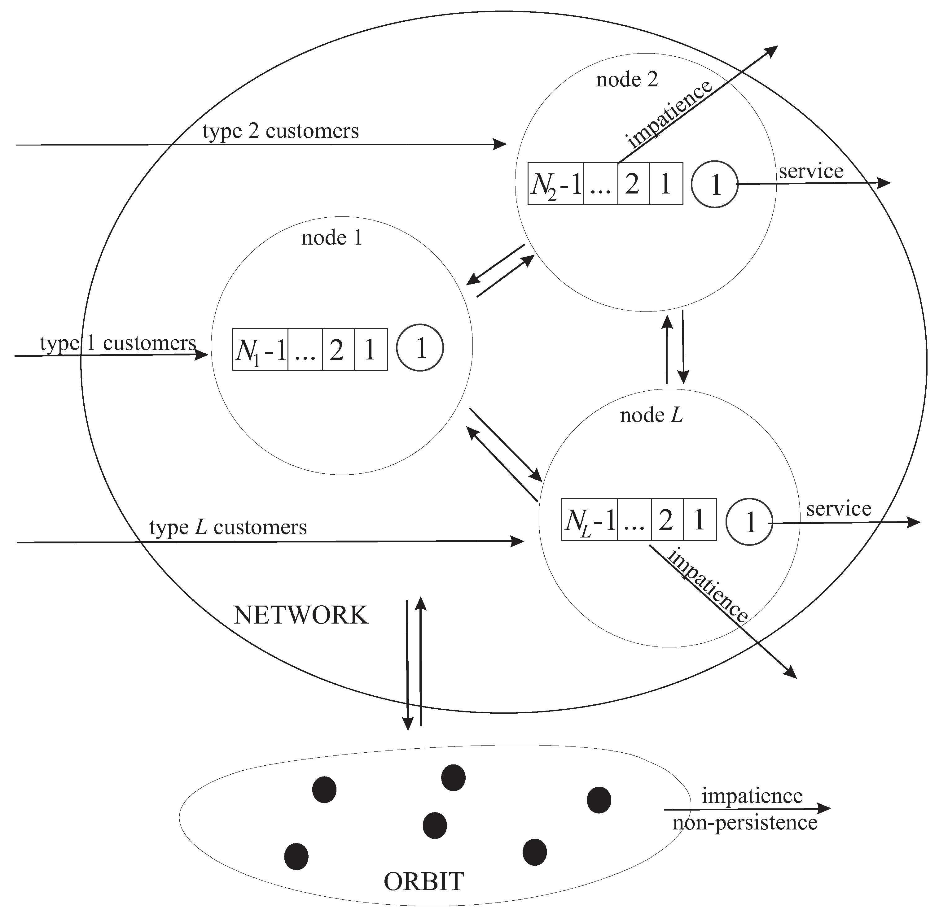
A semi-open queuing network consists of L nodes which are single-server queuing systems with finite buffers. The structure of the network is presented on Figure 1. We assume that the capacity of the buffer at the lth node is equal to $N_l-1,1\le N_l\le \infty .$ The capacity of the network, that is, the maximum number of customers, which can be processed in the network at the same time, is $N,1\le N<\infty .$ We assume that $N\le \underset{l\in \{1,2,\dots ,L\}}{\min }{N}_l.$ This guarantees that customers admitted to the network are not lost during processing in the network due to a buffer overflow.

The admission of arriving (primary) customers to the network is implemented as follows. If the capacity of the network is not exhausted on customer’s arrival, that is, the number of customers in the network is less than $N,$ the customer enters the service. Otherwise, the customer moves to the orbit and retries for service later. The capacity of the orbit is assumed to be infinite. The process of generation of primary customers and retrials of customers from the orbit is defined by the underlying process ${\psi }_t,t\ge 0,$ with a finite state space $\{0,1,\dots ,W\}.$ The intensities of transitions of the process ${\psi }_t$ depend on the current number $i_t$ of customers in the orbit, $i_t\ge 0.$

When $i_t=0,$ that is, the orbit is empty, the intensities of transitions are given by the set of square matrices $D_l,l=\overline{1,L},$ of size $\overline{W}=W+1$ and by the non-diagonal entries of the matrix $D_0.$ Here and thereafter, the notation $l=\overline{1,L}$ means that the parameter l admits the values from the set $\{1,2,\dots ,L\}.$ The diagonal entries of the matrix $D_0$ are negative such as the relation ${\displaystyle \sum _{l=0}^L}{D}_l\mathbf{e}={\mathbf{0}}^T$ holds true where $\mathbf{e}={(1,1,\dots ,1)}^T$, $\mathbf{0}=(0,0,\dots ,0)$ and ${}^T$ is the vector transpose symbol. Transitions, the intensities of which are given by the non-diagonal entries of the matrix $D_0,$ do not cause the generation of primary customers. Transitions, the intensities of which are given by the entries of the matrix $D_l,$ cause the generation of a type-l customer, $l=\overline{1,L}.$ If the capacity of the network is not exhausted at the moment of type-l customer generation, this customer enters the lth node of the network. If the server of this node is idle, the customer starts service. Otherwise, the customer enters the buffer of this node. By comparing the presented description of the arrival process when the orbit is idle with the definition given in Reference [24] we can conclude that this process coincides with the $MMAP.$

Under any fixed number $i,i>0,$ of customers in the orbit, the transitions of the process ${\psi }_t$ can cause either the arrival of a primary customer or a retrial from the orbit. These transitions are given by a set of the same matrices $D_l,l=\overline{0,L},$ and the matrix $D^{(i)}.$ As above, the intensities of transitions, which are given by the entries of the matrix $D_l,$ cause the generation of a primary type-$l,l=\overline{1,L},$ customer. Transitions, the intensities of which are given by the entries of the matrix $D^{(i)},$ cause the generation of a repeated attempt from the orbit. The non-diagonal entries of the matrix $D_0^{(i)}=D_0-\mathrm{diag}\{D^{(i)}\mathbf{e}\}$ define the intensities of transitions which do not cause the generation of primary customers or customers from the orbit. Here, $\mathrm{diag}\{\mathbf{b}\}$ denotes the diagonal matrix with the diagonal entries given by the entries of the vector $\mathbf{b}.$ The matrix ${\displaystyle \sum _{l=1}^L}{D}_l+D^{(i)}+D_0^{(i)}$ is the generator. Let us denote by ${\mathit{\theta }}^{(i)}$ the left stochastic eigenvector of this matrix. Conditional on the fact that i customers are staying in the orbit, the arrival rate of type l primary customers is equal to ${\lambda }_l^{(i)}={\mathit{\theta }}^{(i)}{D}_l\mathbf{e},l=\overline{1,L}.$ The conditional arrival rate of customers from the orbit is equal to ${\lambda }^{(i)}={\mathit{\theta }}^{(i)}{D}^{(i)}\mathbf{e},i>0.$

We assume that customers staying in the orbit are impatient and non-persistent. Impatience means that after a time interval, whose duration is exponentially distributed with parameter $\gamma ,\gamma >0,$ the customer from the orbit leaves the network without service and is lost. The non-persistence means that after unsuccessful retrial attempts, the customer leaves the network forever with probability $h,0\le h\le 1,$ and returns to the orbit with the complementary probability. Analogously, the customers waiting in the buffers of the network are impatient. After the time interval, whose duration is exponentially distributed with the parameter ${\beta }_l,$ a customer waiting in the buffer of the l-th node leaves the node and departs from the network without service.

A retrial customer, which is admitted for service, moves to the l-th node with probability $p_l$, $l=\overline{1,L},{\displaystyle \sum _{l=1}^L}{p}_l=1.$

We assume that the service time at the node l has an exponential distribution with parameter ${\mu }_l,0<{\mu }_l<\infty ,l=\overline{1,L}.$ When this time expires, the serviced customer can move to another node or leave the network forever. The probability of the transition of the serviced customer from the l-th node to the $l^{\prime }$-th node is defined as $q_{l,l^{\prime }},l^{\prime }=\overline{1,L},l^{\prime }\ne l.$ The probability of leaving the network after service in the l-th node is $q_{l,0},q_{l,0}=1-{\displaystyle \sum _{l^{\prime }=1,l^{\prime }\ne l}^L}{q}_{l,l^{\prime }}.$

3. Process of System States

It is easy to see that the dynamics of the considered network is described by the continuous-time Markov chain

$${\xi }_t=\{i_t,n_t,{\psi }_t,n_t^{(1)},\dots ,n_t^{(L)}\},t\ge 0,$$

where, at the moment $t,t\ge 0,$

• $i_t$ is the number of customers in the orbit, $i_t\ge 0;$
• $n_t$ is the total number of customers in the network, $n_t=\overline{0,N};$
• ${\psi }_t$ is the state of the underlying process of the arrival process of primary and retrial customers, ${\psi }_t=\overline{0,W};$
• $n_t^{(l)}$ is the number of customers in the l-th node, $l=\overline{1,L},$ $n_t^{(l)}=\overline{0,n_t},$${\displaystyle \sum _{l=1}^L}{n}_t^{(l)}=n_t.$

To compute the stationary distribution of the states of the Markov chain ${\xi }_t,t\ge 0,$ we need to derive the generator of this chain. To this end, we use the matrix-analytic methods. Therefore, to simplify derivation of the generator it is useful to deal not with separate states of the chain but with whole groups of the states having the same value of the two first components of the Markov chain. We call such a group having the value $(i,n)$ of these components a macro-state $(i,n)$. There are many possibilities to enumerate the states of the Markov chain that belong to a fixed macro-state. Here, we assume that the states are numerated in the reverse lexicographic order of the components $n_t^{(1)},\dots ,n_t^{(L)}$ and the direct lexicographic order of the component ${\psi }_t.$ We call the set of macro-states $\{(i,0),(i,1),\dots ,(i,N)\}$ as the level $i,i\ge 0.$

To simplify derivations, in what follows, we use the following notation:

• I is the identity matrix and O is a zero matrix of an appropriate dimension;
• ⊗ and ⊕ are the symbols of Kronecker product and sum of matrices, respectively, see Reference [26];
• $\mathrm{diag}\{\dots \}$ is the diagonal matrix with the diagonal entries listed or defined by the entries of the vector in the brackets;
• ${\mathrm{diag}}_{+}\{\dots \}$ is the updiagonal matrix with the updiagonal entries listed in the brackets;
• ${\mathrm{diag}}_{-}\{\dots \}$ is the subdiagonal matrix with the subdiagonal entries listed in the brackets;
• $\mathit{\beta }$ is the column vector defined as $\mathit{\beta }={({\beta }_1,\dots ,{\beta }_L)}^T;$
• $\mathbf{p}$ is the row vector defined as $\mathbf{p}=(p_1,\dots ,p_L);$
• ${\mathbf{a}}_l$ is the row vector of size L that has all zero components except the lth component which is equal to 1;
• $\mathbf{q}$ is the column vector defined as $\mathbf{q}={(q_1,q_2,\dots ,q_L)}^T={(q_{1,0}{\mu }_1,q_{2,0}{\mu }_2,\dots ,q_{L,0}{\mu }_L)}^T$;
• $T_n=\left(\genfrac{}{}{0pt}{}{n+L-1}{L-1}\right)=\frac{(n+L-1)!}{n!(L-1)!}$ is the number of states of the process $(n_t^{(1)},\dots ,n_t^{(L)})$ when ${\displaystyle \sum _{l=1}^L}{n}_t^{(l)}=n,n=\overline{0,N}.$

Because we will operate with macro-states, we need to analyse the vector process ${\mathbf{n}}_t=\{n_t^{(1)},\dots ,n_t^{(L)}\},$$t\ge 0,$ that defines the dynamics of the number of customers in the nodes of the network. The following events can change this number:

(1)

An admission to the network of a customer from the orbit. Let us denote as $P_n(\mathbf{p}),n=\overline{0,N-1},$ the matrix consisting of probabilities of the transitions of the process ${\mathbf{n}}_t$ during the epoch when $n,n<N,$ customers are obtaining service in the network and a customer from the orbit makes a retrial attempt;

(2)

An admission to the network of an arriving type-l customer. Let us denote as $P_n({\mathbf{a}}_l),n=\overline{0,N-1},$ the matrix consisting of the transitions probabilities of the process ${\mathbf{n}}_t$ during the epoch when $n,n<N,$ customers are obtaining service in the network and a type-l customer arrives to the system;

(3)

A customer finishes the service in one of the nodes and transits to some another one. Let us denote as $B_n,n=\overline{1,N},$ the matrix which components define the intensities of the process ${\mathbf{n}}_t$ transitions in this case, conditioned on the fact that n customers are in the network;

(4)

A customer finishes the service in some node and leaves the network. Let us denote as $S_n(\mathbf{q}),n=\overline{0,N-1},$ the matrix which components define the intensities of the process ${\mathbf{n}}_t$ transitions in this case, conditioned on the fact that there are $N-n$ customers in the network;

(5)

A customer leaves some node due to impatience. The matrix $Z_n(\mathit{\beta }),n=\overline{1,N},$ defines the intensities of the process ${\mathbf{n}}_t$ transitions in the considered case when there are n customers in the network.

It is worth noting that the matrices $P_n,S_n(\mathbf{q}),n=\overline{0,N-1},$ and $B_n,n=\overline{1,N},$ can be computed based on the use of the corresponding results from Reference [10]. Derivation of matrices $Z_n(\mathit{\beta })$ is novel because the impatience of the customers staying in the buffers of the network nodes was not considered in the related literature previously. This derivation can be performed as follows.

Step (1)

We compute the matrices $Z_n^{(k)}(\mathit{\beta })$ using the recursive formulas:

$$Z_n^{(0)}(\mathit{\beta })=(n-1){\beta }_L,n=\overline{1,N},$$

$$Z_n^{(k)}(\mathit{\beta })=\left(\begin{array}{cccc}(n-1){\beta }_{L-k}I& O& \dots & O\\ Z_1^{(k-1)}(\mathit{\beta })& (n-2){\beta }_{L-k}I& \dots & O\\ O& Z_2^{(k-1)}(\mathit{\beta })& \dots & O\\ ⋮& ⋮& \ddots & ⋮\\ O& O& \dots & 0{\beta }_{L-k}I\\ O& O& \dots & Z_n^{(k-1)}(\mathit{\beta })\end{array}\right),k=\overline{1,L-1},n=\overline{1,N}.$$

Step (2)

Compute the matrices $Z_n(\mathit{\beta })$ as $Z_n(\mathit{\beta })=Z_n^{(L-1)}(\mathit{\beta }),n=\overline{0,N-1}.$

Also, let us introduce the matrix ${\Gamma }_n.$ It is the diagonal matrix the diagonal entries of which define the intensities of exit of the process ${\mathbf{n}}_t$ from its states when n customers obtain service in the network. The matrices ${\Gamma }_n$ are defined as follows:

$${\Gamma }_0=0,{\Gamma }_n=-\mathrm{diag}\{B_n\mathbf{e}+S_{N-n}(\mathbf{q})\mathbf{e}+Z_n(\beta )\mathbf{e}\},n=\overline{1,N}.$$

We denote as $\mathbf{G}$ the infinitesimal generator of the Markov chain ${\xi }_t,t\ge 0.$ The matrix $\mathbf{G}$ has an infinite size. It consists of the blocks ${\mathbf{G}}_{i,j},i,j\ge 0,$ defining transition intensities from the level i to the level $j.$ In turn, each matrix ${\mathbf{G}}_{i,j}$ consists of sub-blocks ${\mathbf{G}}_{i,j}^{(n,n^{\prime })}$ of transition intensities from the macro-state $(i,n)$ to the macro-state $(j,n^{\prime }).$ The diagonal entries of the blocks ${\mathbf{G}}_{i,i}^{(n,n)}$ are negative and are equal, up to the sign, to the rates of the exit of the Markov chain ${\xi }_t$ from the corresponding states.

Lemma 1.

The infinitesimal generator $\mathbf{G}$ of the Markov chain ${\xi }_t,t\ge 0,$ has a block-tridiagonal structure:

$$\begin{array}{c}\hfill \mathbf{G}=\mathrm{diag}\{{\mathbf{G}}_{i,i},i\ge 0\}+{\mathrm{diag}}_{+}\{{\mathbf{G}}_{i,i+1},i\ge 0\}+{\mathrm{diag}}_{-}\{{\mathbf{G}}_{i,i-1},i\ge 1\}.\end{array}$$

(1)

The non-zero blocks ${\mathbf{G}}_{i,j},i,j\ge 0,$ have the following form:

$${\mathbf{G}}_{i,i}=\mathrm{diag}\{{\mathbf{G}}_{i,i}^{(n,n)},n=\overline{0,N}\}+{\mathrm{diag}}_{+}\{{\mathbf{G}}_{i,i}^{(n,n+1)},n=\overline{0,N-1}\}+{\mathrm{diag}}_{-}\{{\mathbf{G}}_{i,i}^{(n,n-1)},n=\overline{1,N}\},i\ge 0,$$

(2)

$${\mathbf{G}}_{i,i-1}=\mathrm{diag}\{{\mathbf{G}}_{i,i-1}^{(n,n)},n=\overline{0,N}\}+{\mathrm{diag}}_{+}\{{\mathbf{G}}_{i,i-1}^{(n,n+1)},n=\overline{0,N-1}\},i\ge 1,$$

(3)

$${\mathbf{G}}_{i,i+1}=\mathrm{diag}\{O,\dots ,O,{\displaystyle \sum _{k=1}^L}{D}_k\otimes I_{T^N}\},i\ge 0,$$

(4)

where

$${\mathbf{G}}_{i,i}^{(0,0)}=D_0^{(i)}-i\gamma I_{\overline{W}},$$

(5)

$${\mathbf{G}}_{i,i}^{(n,n)}=(D_0^{(i)}-i\gamma I_{\overline{W}})\oplus (B_n+{\Gamma }_n),n=\overline{1,N-1},$$

(6)

$${\mathbf{G}}_{i,i}^{(N,N)}=(D_0^{(i)}+(1-h)D^{(i)}-i\gamma I_{\overline{W}})\oplus (B_N+{\Gamma }_N),$$

(7)

$${\mathbf{G}}_{i,i}^{(n,n+1)}={\displaystyle \sum _{k=1}^L}{D}_k\otimes P_n({\mathbf{a}}_k),n=\overline{0,N-1},$$

(8)

$${\mathbf{G}}_{i,i}^{(n,n-1)}=I_{\overline{W}}\otimes (S_{N-n}(\mathbf{q})+Z_n(\beta )),n=\overline{1,N},$$

(9)

$${\mathbf{G}}_{i,i-1}^{(n,n+1)}=D^{(i)}\otimes P_n(\mathbf{p}),n=\overline{0,N-1},$$

(10)

$${\mathbf{G}}_{i,i-1}^{(n,n)}=i\gamma I_{\overline{W}{T}_n},n=\overline{0,N-1},$$

(11)

$${\mathbf{G}}_{i,i-1}^{(N,N)}=i\gamma I_{\overline{W}{T}_N}+h{D}^{(i)}\otimes I_{T_N}.$$

(12)

A brief proof of the Lemma is as follows. Block tridiagonal structure (1) of the generator $\mathbf{G}$ is explained by the fact that the probability of two or more customers arrival or departure from the orbit during the interval of the infinitesimal length is negligible. The matrices ${\mathbf{G}}_{i,i},{\mathbf{G}}_{i,i-1},{\mathbf{G}}_{i,i+1}$ have block structures (2)–(4) were the blocks define the intensities of transitions that lead to the corresponding change of the number of customers presenting in the network.

The most simple form (4) has the matrix ${\mathbf{G}}_{i,i+1}$ defining the intensities of customers arriving at the orbit. Because a customer joins the orbit only when the capacity of the server is exhausted (the number of customers in the network is equal to N), only one block of the matrix ${\mathbf{G}}_{i,i+1},$ namely, ${\mathbf{G}}_{i,i+1}^{(N,N)},$ is not equal to zero. This matrix block corresponds to the arrival of a primary customer of any type when the number of customers in the network is equal to $N.$ This customer moves to the orbit and the number of customers in the network does not change.

The matrix ${\mathbf{G}}_{i,i-1}$ defining the intensities of customers departure from the orbit is the block two-diagonal matrix of form (3). It has the non-zero diagonal blocks corresponding to the case when the customer departing from the orbit does not enter the network but is lost. Such a departure occurs due to the impatience of the customers in the orbit when the number of customers in the network is equal to n, $n<N,$ or the impatience and non-persistence of the customers staying in the orbit when this number is equal to $N.$ The corresponding intensities of the departure are given by the matrices of form (11) and (12), respectively. The matrix ${\mathbf{G}}_{i,i-1}$ has also the up-diagonal blocks corresponding to the case when a customer from the orbit makes a retrial when the number of customers in the network is equal to n, $n<N,$ and enters the network. After entering the network, this customer joins some of the network nodes. The intensities of occurrence of these events are given by the matrices of form (10).

The matrix ${\mathbf{G}}_{i,i}$ has block tridiagonal structure (2). The diagonal entries of its diagonal blocks ${\mathbf{G}}_{i,i}^{(n,n)}$ are negative. Their values with the opposite sign define the rate of the exit of the Markov chain ${\xi }_t$ from the corresponding states. These diagonal entries are the corresponding entries of the matrices of form (5), if $n=0$, (6), if $n=\overline{1,N-1},$ and (7) if $n=N.$ The non-diagonal entries of the diagonal blocks ${\mathbf{G}}_{i,i}^{(n,n)}$ are non-negative and define the intensities of the transitions of the Markov chain ${\xi }_t$ that do not cause the change of the number of customers neither in the orbit and in the network. These entries are given by the corresponding entries of the matrices of form (5), if $n=0$, (6), if $n=\overline{1,N-1},$ and (7) if $n=N.$ The up-diagonal blocks ${\mathbf{G}}_{i,i}^{(n,n+1)}$ correspond to the arrival of a primary customer of any type when the number of the customers in the network is less than N and its entering the corresponding node of the network. These blocks are defined by formula (8). The sub-diagonal blocks ${\mathbf{G}}_{i,i}^{(n,n-1)}$ correspond to a customer departure from the network due to the service completion or due to impatience and have the form (9). Lemma is proven.

It can be shown that the Markov chain ${\xi }_t,t\ge 0,$ belongs to the class of Asymptotically Quasi-Toeplitz Markov chains, see Reference [27]. Using the results from Reference [27], it is easily verified that because the customers in orbit are impatient, that is, $\gamma >0$, the Markov chain ${\xi }_t,t\ge 0,$ is ergodic. Then, the following limits (stationary probabilities) exist for any set of the network parameters:

$$\pi (i,n,\psi ,n^{(1)},\dots ,n^{(L)})=\underset{t\to \infty }{\lim }P\{i_t=i,n_t=n,{\psi }_t=\psi ,n_t^{(1)}=n^{(1)},\dots ,n_t^{(L)}=n^{(L)}\},$$

$$i\ge 0,n=\overline{0,N},\psi =\overline{0,W},n^{(l)}=\overline{0,n},l=\overline{1,L},{\displaystyle \sum _{l=1}^L}{n}^{(l)}=n.$$

Let us denote by $\pi (i,n)$ the row vectors of the stationary probabilities that belong to the macro-state $(i,n)$ and by ${\pi }_i$ the row vectors of the stationary probabilities that belong to the level $i,i\ge 0.$

It is well known that the probability vectors ${\pi }_i,i\ge 0,$ satisfy the following system of linear algebraic equations:

$$({\pi }_0,{\pi }_1,\dots )\mathbf{G}=\mathbf{0},({\pi }_0,{\pi }_1,\dots )\mathbf{e}=1.$$

(13)

Comparing this system with the corresponding system for the probability vectors ${\pi }_i,i\ge 0,$ for the analogous queuing network with the buffer considered in Reference [10], we see the following. The size of the vectors ${\pi }_i$ (and the size of the corresponding square blocks of the generator) in Reference [10] is equal to $\overline{W}{T}_i$ if $i=\overline{0,N},$ and $\overline{W}{T}_N$ if $i>N.$ The size of all vectors ${\pi }_i,i\ge 0,$ in the considered in our paper model of the queuing network with retrials is equal to $\overline{W}{\displaystyle \sum _{n=0}^N}{T}_n.$ Therefore, the blocks of generator (1) are much larger than the blocks of the generator in Reference [10]. Thus, the algorithm from Reference [28], which was used for numerical work in Reference [10], is not very effective for solving system (13). To solve this system, we recommend to use a more effective numerically stable algorithm recently developed in Reference [29].

4. Performance Measures

The average number $N_{orbit}$ of customers in the orbit is computed by

$$N_{orbit}={\displaystyle \sum _{i=1}^{\infty }}i{\pi }_i\mathbf{e}.$$

The average number $N_{network}$ of customers in the network at an arbitrary moment is computed by

$$N_{network}={\displaystyle \sum _{i=0}^{\infty }}{\displaystyle \sum _{n=1}^N}n\pi (i,n)\mathbf{e}.$$

The probability $P_{imm}$ that an arbitrary customer is admitted to the network immediately upon arrival is computed by

$$P_{imm}=\frac{{\displaystyle \sum _{i=0}^{\infty }}{\displaystyle \sum _{n=0}^{N-1}}\pi (i,n)(\widehat{D}\otimes I_{T_n})\mathbf{e}}{\widehat{\lambda }}$$

where the average arrival rate of primary customers $\widehat{\lambda }$ is computed by

$$\widehat{\lambda }={\displaystyle \sum _{i=0}^{\infty }}{\displaystyle \sum _{n=0}^N}\pi (i,n)(\widehat{D}\otimes I_{T_n})\mathbf{e}$$

and $\widehat{D}={\displaystyle \sum _{r=1}^L}{D}_r.$

Remark 1.

If all the matrices $D^{(i)}$ are the diagonal, that is, the underlying process ${\psi }_t$ of arrivals cannot make the jumps into other states at the moments of retrials, then the average arrival rate of primary customers $\widehat{\lambda }$ is equal to the arrival rate λ of the $MMAP$ that arrives at time intervals when the orbit is empty. The value λ is given by $\lambda =\theta \widehat{D}\mathbf{e}$ where the row vector θ is the unique solution of the system $\theta (D_0+\widehat{D})=\mathbf{0},\theta \mathbf{e}=1.$ If some of the matrices $D^{(i)}$ are non-diagonal, then generally speaking $\widehat{\lambda }\ne \lambda .$

The average intensity ${\lambda }_{out-serve}^{(l)}$ of flow of customers who leave the network after successful service from the l-th node is computed by

$${\lambda }_{out-serve}^{(l)}={\displaystyle \sum _{i=0}^{\infty }}{\displaystyle \sum _{n=1}^N}\pi (i,n)(I_{\overline{W}}\otimes S_{N-n}({\mathbf{q}}^{(l)}))\mathbf{e},l=\overline{1,L},$$

where ${\mathbf{q}}^{(l)}$ is a column vector of size L with all zero components except the component ${({\mathbf{q}}^{(l)})}_l=q_l.$

The average intensity ${\lambda }_{out-serve}$ of flow of customers who leave the network after successful service is computed by

$${\lambda }_{out-serve}={\displaystyle \sum _{i=0}^{\infty }}{\displaystyle \sum _{n=1}^N}\pi (i,n)(I_{\overline{W}}\otimes S_{N-n}(\mathbf{q}))\mathbf{e}.$$

The average intensity ${\lambda }_{out-imp}^{(l)}$ of flow of customers who leave the network due to impatience from the l-th node is computed by

$${\lambda }_{out-imp}^{(l)}={\displaystyle \sum _{i=0}^{\infty }}{\displaystyle \sum _{n=2}^N}\pi (i,n)(I_{\overline{W}}\otimes Z_n({\beta }^{(l)}))\mathbf{e},l=\overline{1,L},$$

where ${\mathit{\beta }}^{(l)}$ is a column vector of size L with all zero components except the component ${({\mathit{\beta }}^{(l)})}_l={\beta }_l.$

The average intensity ${\lambda }_{out-imp}$ of flow of customers who leave the network due to impatience is computed by

$${\lambda }_{out-imp}={\displaystyle \sum _{i=0}^{\infty }}{\displaystyle \sum _{n=2}^N}\pi (i,n)(I_{\overline{W}}\otimes Z_n(\mathit{\beta }))\mathbf{e}.$$

The probability of an arbitrary customer loss due to impatience from the orbit is computed by

$$P_{loss}^{imp-orbit}={\widehat{\lambda }}^{-1}\gamma N_{orbit}.$$

The probability of an arbitrary customer loss due to non-persistence from the orbit is computed by

$$P_{loss}^{nonpersist-orbit}={\widehat{\lambda }}^{-1}h{\displaystyle \sum _{i=1}^{\infty }}\pi (i,N)(D^{(i)}\otimes I_{T_N})\mathbf{e}.$$

The probability of an arbitrary customer loss due to impatience from the network is computed by

$$P_{loss}^{imp-net}={\widehat{\lambda }}^{-1}{\lambda }_{out-imp}.$$

The probability of an arbitrary customer loss due to impatience from the lth node of the network is computed by

$$P_{loss}^{imp-net,l}={\widehat{\lambda }}^{-1}{\lambda }_{out-imp}^{(l)},l=\overline{1,L}.$$

The probability of an arbitrary customer loss is computed by

$$P_{loss}=1-\frac{{\lambda }_{out-serve}}{\widehat{\lambda }}=P_{loss}^{imp-orbit}+P_{loss}^{imp-net}+P_{loss}^{nonpersist-orbit}.$$

The average intensity ${\mu }_{out}^{(l)}$ of output flow of successfully served customers from the l-th node is computed by

$${\mu }_{out}^{(l)}={\displaystyle \sum _{i=0}^{\infty }}{\displaystyle \sum _{n=1}^N}\pi (i,n)(I_{\overline{W}}\otimes S_{N-n}({\mathbf{m}}^{(l)}))\mathbf{e},l=\overline{1,L},$$

where ${\mathbf{m}}^{(l)}$ is the column vector of size L with all zero components except the component ${({\mathbf{m}}^{(l)})}_l={\mu }_l.$

The load of the l-th node ${\rho }_l$ can be found as follows:

$${\rho }_l=\frac{{\mu }_{out}^{(l)}}{{\mu }_l(1-P_{loss}^{imp-net,l})},l=\overline{1,L}.$$

This characteristic of the node operation is very important because knowledge of its value is helpful to recognize the so-called bottlenecks in the network and to make certain managerial updates.

5. Numerical Examples

We present the results of three numerical experiments. In the first experiment, we illustrate the importance on account of possible dependence of arrival processes of primary and retrial customers. The aim of the second experiment is the numerical investigation of the dependence of the main performance measures of the system on the threshold N and illustration of the importance of account the impatience of customers staying in the network. In the third experiment, we show how our results can be used for localization of the bottlenecks of the network and improvement of the performance of the network via upgrading the bottleneck node.

Remark 2.

The importance of correlation in the arrival process for a similar queuing network without retrials was shown in Reference [10]. In this paper, we do not present the results illustrating the importance of the correlation. We mention only that the correlation in the arrival process of primary customers has an essential impact on the networks with retrials as well.

Example 1.

Let us consider a queuing network consisting of $L=3$ nodes. The mean service rates at these nodes are ${\mu }_1=2,{\mu }_2=1.5,{\mu }_3=2,$ respectively.

The transition probabilities of the customers in the network $q_{l,k},l=\overline{1,L},k=\overline{0,L},k\ne l,$ are defined as the corresponding entries of

Table 1. Transition probabilities $q_{l,k}$.

${\mathit{q}}_{\mathit{l},\mathit{k}}$	$\mathit{k}=0$	$\mathit{k}=1$	$\mathit{k}=2$	$\mathit{k}=3$
$l=1$	$\frac{1}{2}$	-	$\frac{1}{4}$	$\frac{1}{4}$
$l=2$	$\frac{1}{3}$	$\frac{2}{15}$	-	$\frac{8}{15}$
$l=3$	$\frac{1}{2}$	$\frac{1}{4}$	$\frac{1}{4}$	-

.

The probabilities defining the choice of the node at the moment of admission of a customer from the orbit are chosen as: $p_1=0.2,p_2=0.3,$ and $p_3=0.5.$ The intensity of impatience of a customer from the orbit is assumed to be $\gamma =0.02.$ The probability of a customer departure from the orbit after an unsuccessful retrial is $h=0.3.$ The intensities of impatience of customers from the nodes are given as follows: ${\beta }_1=0.05,{\beta }_2=0.01,{\beta }_2=0.03.$

We assume that the $MMAP$ arrival flow of primary customers when the orbit is empty is defined by the following matrices:

$$D_0=\left(\begin{array}{cc}-1.764& 0.014\\ 0.07& -0.42\end{array}\right),D_1=\left(\begin{array}{cc}0.07& 0.007\\ 0& 0.14\end{array}\right),$$

$$D_2=\left(\begin{array}{cc}0.028& 0.035\\ 0.0042& 0.203\end{array}\right),D_3=\left(\begin{array}{cc}1.603& 0.007\\ 0.0021& 0.0007\end{array}\right).$$

The retrial rates of customers from the orbit when i customers are staying in the orbit are defined by the entries of the matrix

$$D^{(i)}=i\tilde{D},$$

where

$$\tilde{D}=\left(\begin{array}{cc}0.2& 0\\ 0& 0.02\end{array}\right).$$

Remark 3.

We intentionally choose the matrix $D^{(i)}$ in the simple diagonal form. This allows us to calculate the average individual retrial rate α of a customer from the orbit as

$$\alpha =\sigma \tilde{D}\mathbf{e},$$

where σ is the unique solution of the following system

$$\sigma (D_0+{\displaystyle \sum _{l=1}^L}{D}_l-\mathrm{diag}\{\tilde{D}\mathbf{e}\})=\mathbf{0},\sigma \mathbf{e}=1.$$

In this example, α is equal to $0.1185929648$.

In the considered model, the arrival flows of primary and retrials customers are dependent. In the existing literature, such dependence was not analyzed. In this example, we clarify whether or not this dependence is essential. To this end, we also consider the case when customers in the orbit retry to obtain access to the network independently on primary customers as assumed in the existing literature. We suppose that each customer from the orbit makes repeated attempts with the intensity $\alpha =0.1185929648.$

It is easy to see that the results for the model with independent flows of primary and retrial customers are obtained as the particular case of our results if we assume that the matrix $\tilde{D}$ has the following form:

$$\tilde{D}=\left(\begin{array}{cc}\alpha & 0\\ 0& \alpha \end{array}\right).$$

Let us vary the number N of customers, which can be serviced in the network simultaneously, over the interval $[1,15].$ The computations were performed on a PC with an Intel Core i7-8700 CPU and 16 GB RAM. The computation time for all N from 1 to 15 is about 4 min and 50 s.

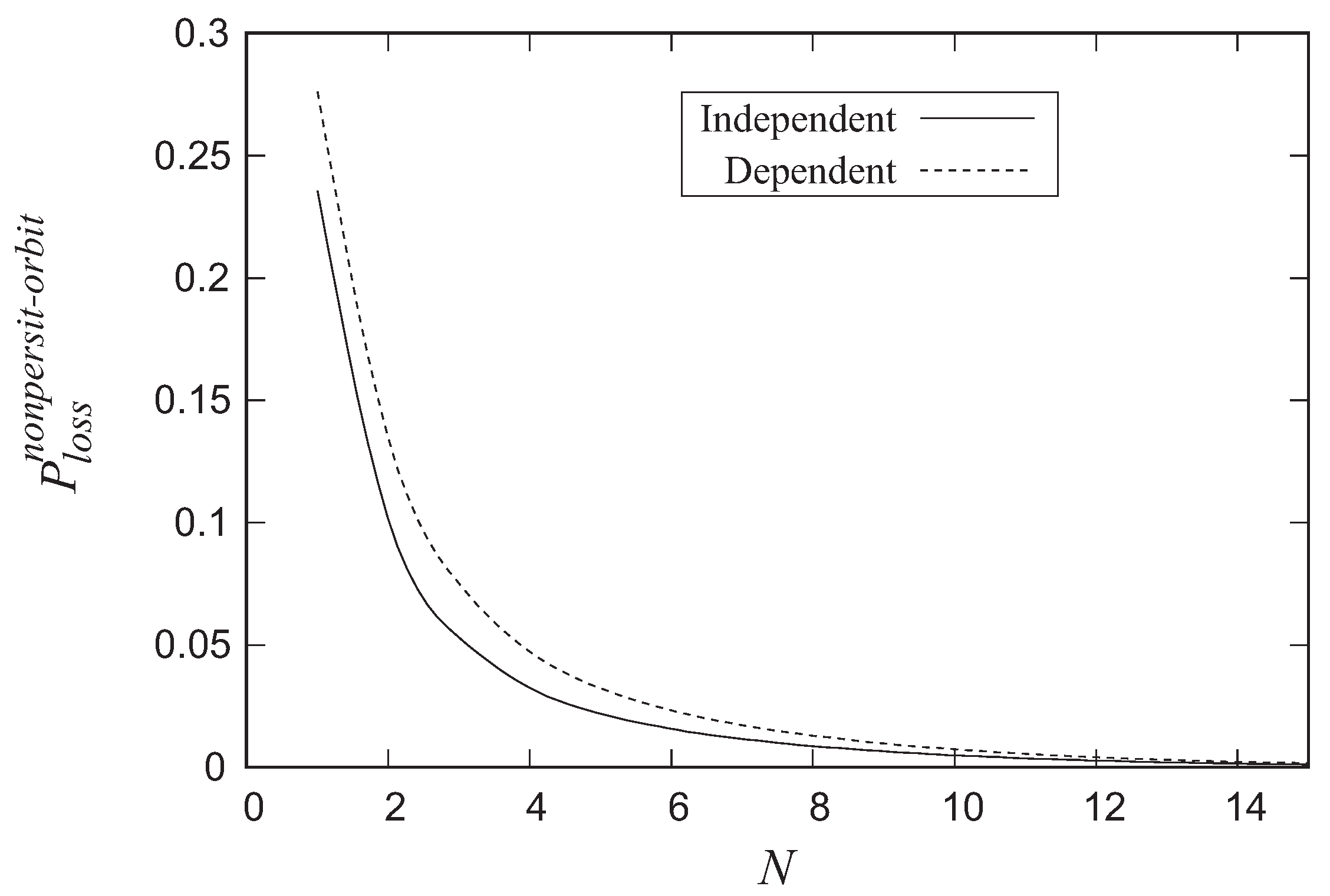
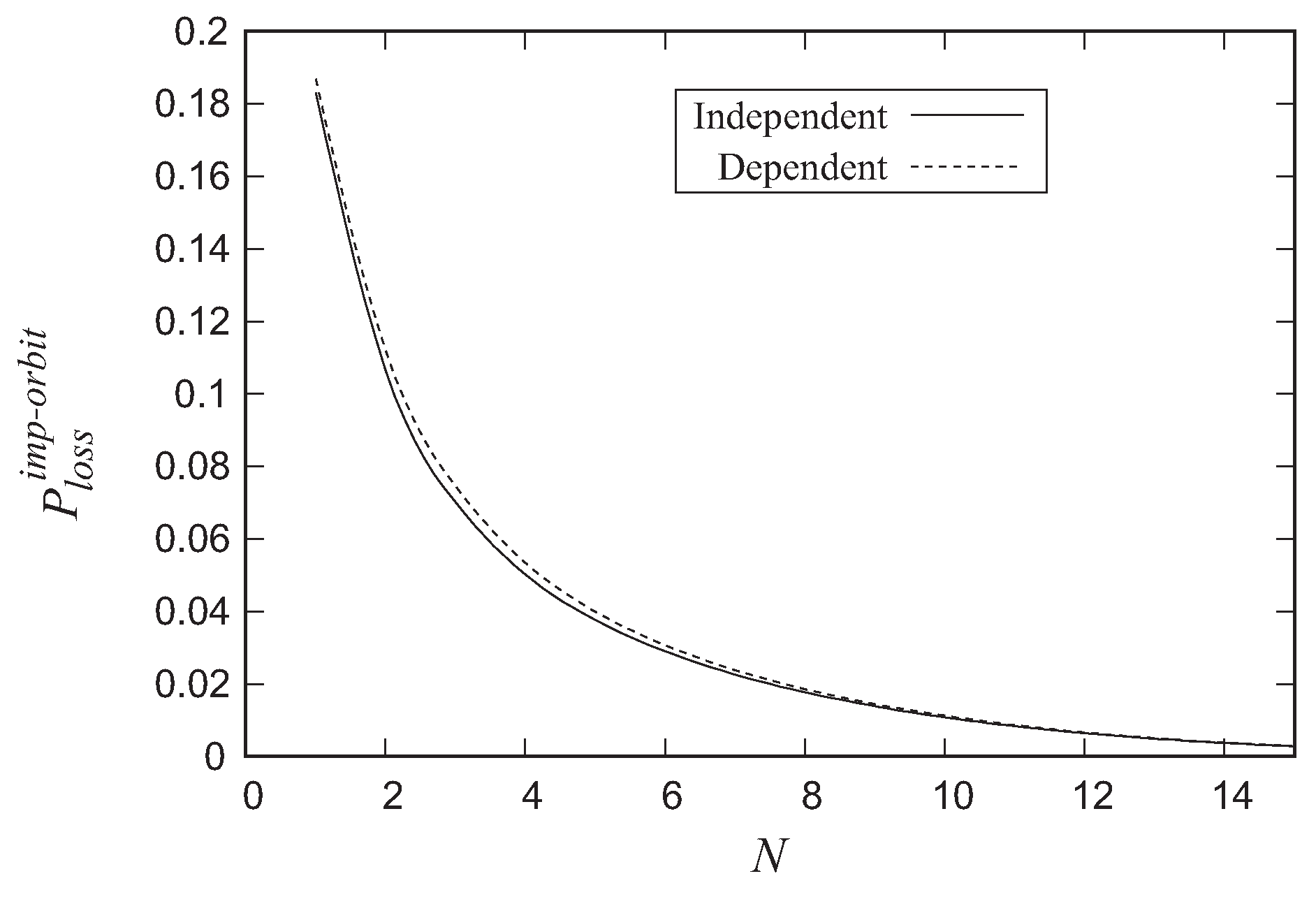
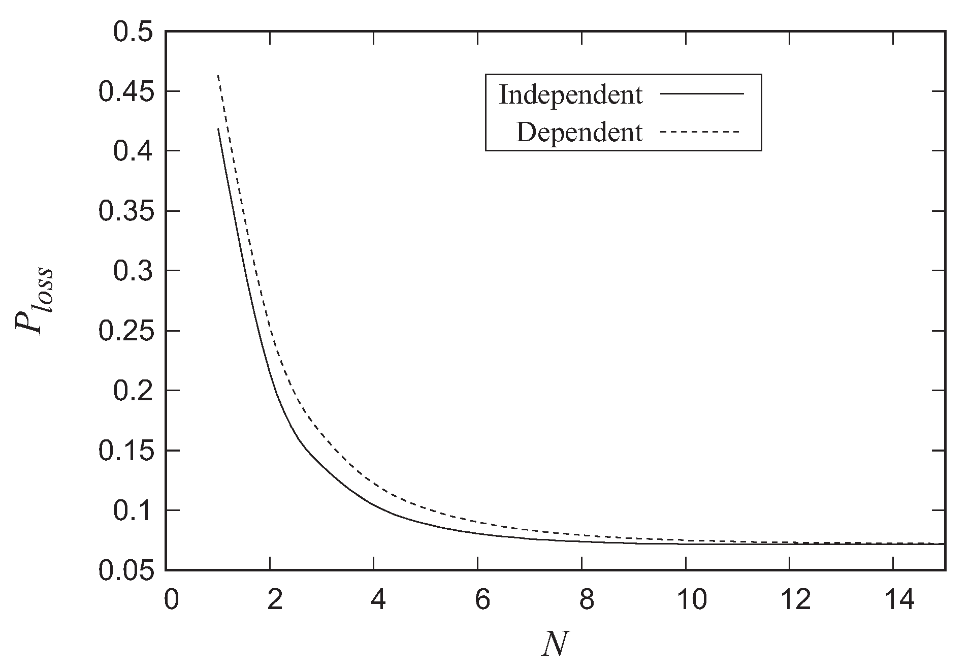
Figure 2, Figure 3 and Figure 4 illustrate the dependence on N of the probability of an arbitrary customer loss due to non-persistence from the orbit $P_{loss}^{nonpersist-orbit}$, due to impatience from the orbit $P_{loss}^{imp-orbit}$ and the loss probability of an arbitrary customer $P_{loss}$ for the systems with dependent and independent arrivals of primary and retrial customers.

As it is seen from these figures, an account of the dependence of arrivals of primary and retrial customers is important for the precious prediction of the system performance measures. Under the chosen values of the network parameters, this dependence deteriorates the performance of the network. All loss probabilities are greater when the flows are dependent. In this example, the error in the estimation the loss probabilities can be up to 20% on their real values.

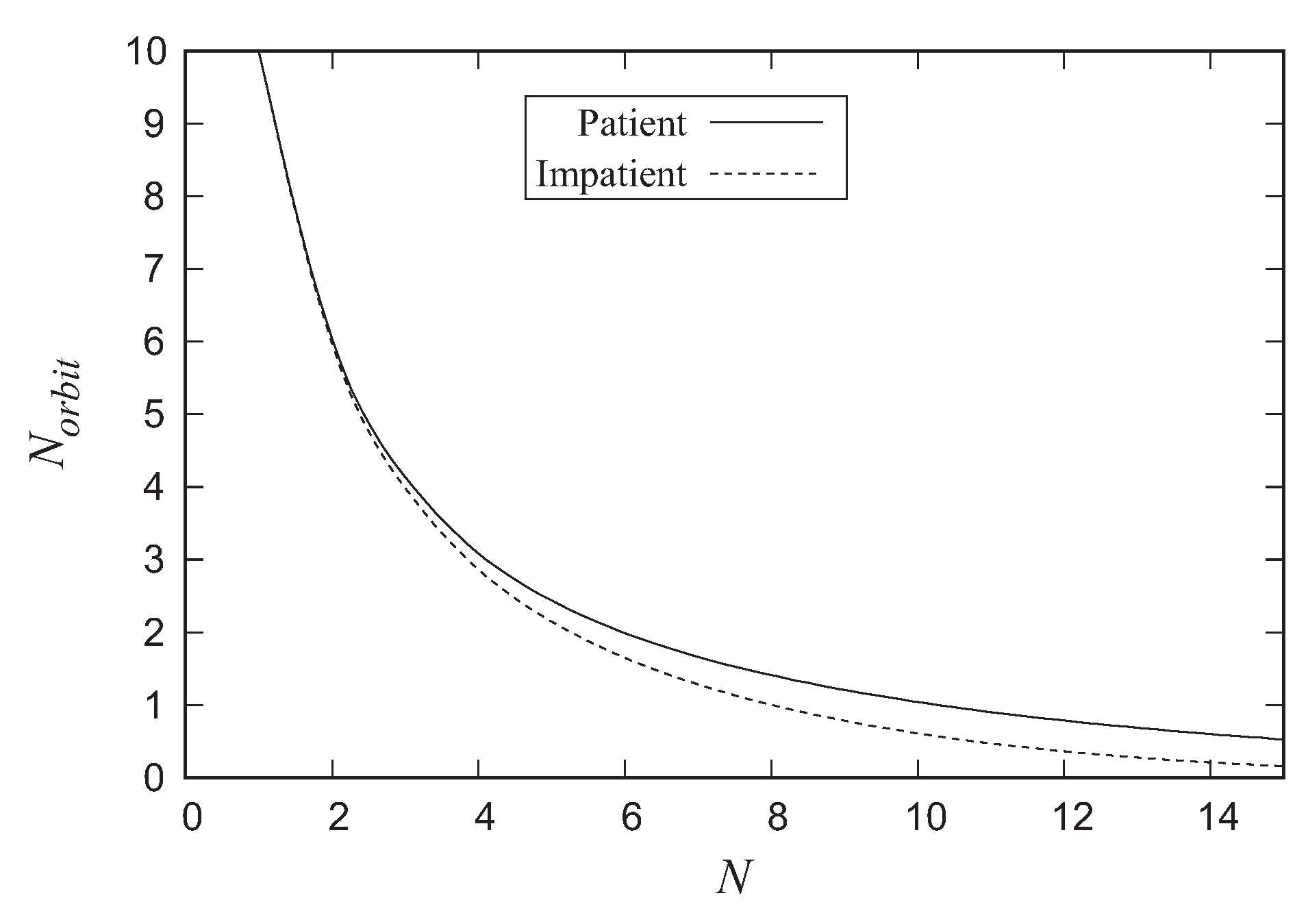
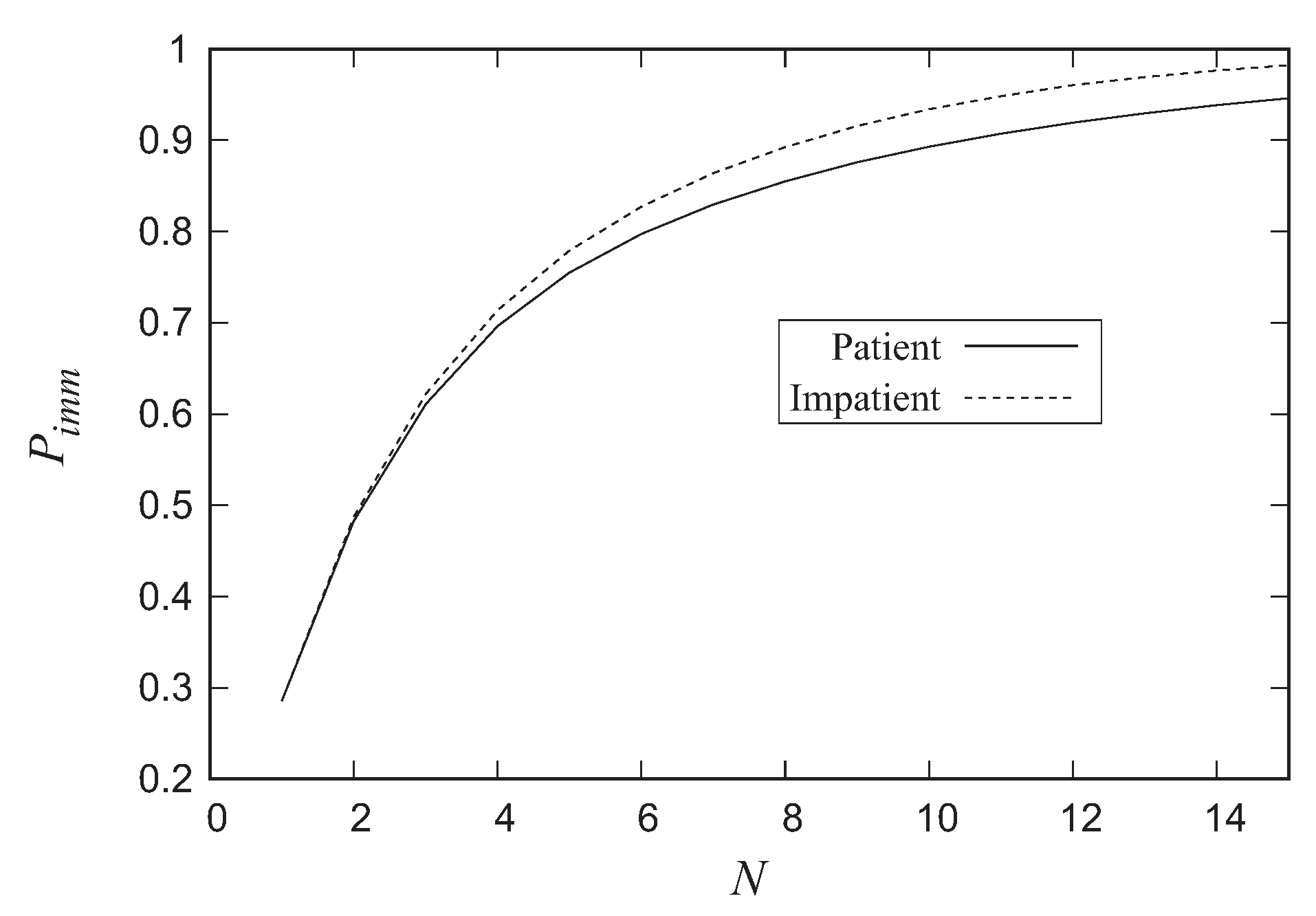
Example 2.

In this example, we numerically investigate the dependence of the main performance measures of the system on the threshold $N.$ We also investigate the importance of accounting the impatience of customers in the nodes of the network. Let us assume that all system parameters are the same as in the previous example except for the matrix

$$\tilde{D}=\left(\begin{array}{cc}0.2& 0.002\\ 0.001& 0.02\end{array}\right).$$

In the previous example, we chose relatively small intensities of impatience of customers from the nodes: ${\beta }_1=0.05,{\beta }_2=0.01,{\beta }_2=0.03.$ The question arises, whether or not it is possible to ignore such small intensities of impatience and assume that the customers are patient, that is, ${\beta }_l=0,l=\overline{1,L}.$

Figure 5, Figure 6 and Figure 7 illustrate the dependence on N of the average number $N_{orbit}$ of customers in the orbit, the probability $P_{imm}$ that an arbitrary customer is admitted to the network immediately upon arrival and the probability of an arbitrary customer loss due to impatience from the network $P_{loss}^{imp-net}$ for the cases of the patient and impatient customers in the nodes of the network.

The probability of an arbitrary customer loss due to impatience from the network $P_{loss}^{imp-net}$ is equal to 0 when the customers in the nodes are patient and essentially increases with the growth of N when the customers are impatient. It is worth to note that the loss of the customers due to impatience in the nodes causes the reduction of the average number of customers in the orbit and the increase of the probability $P_{imm}.$

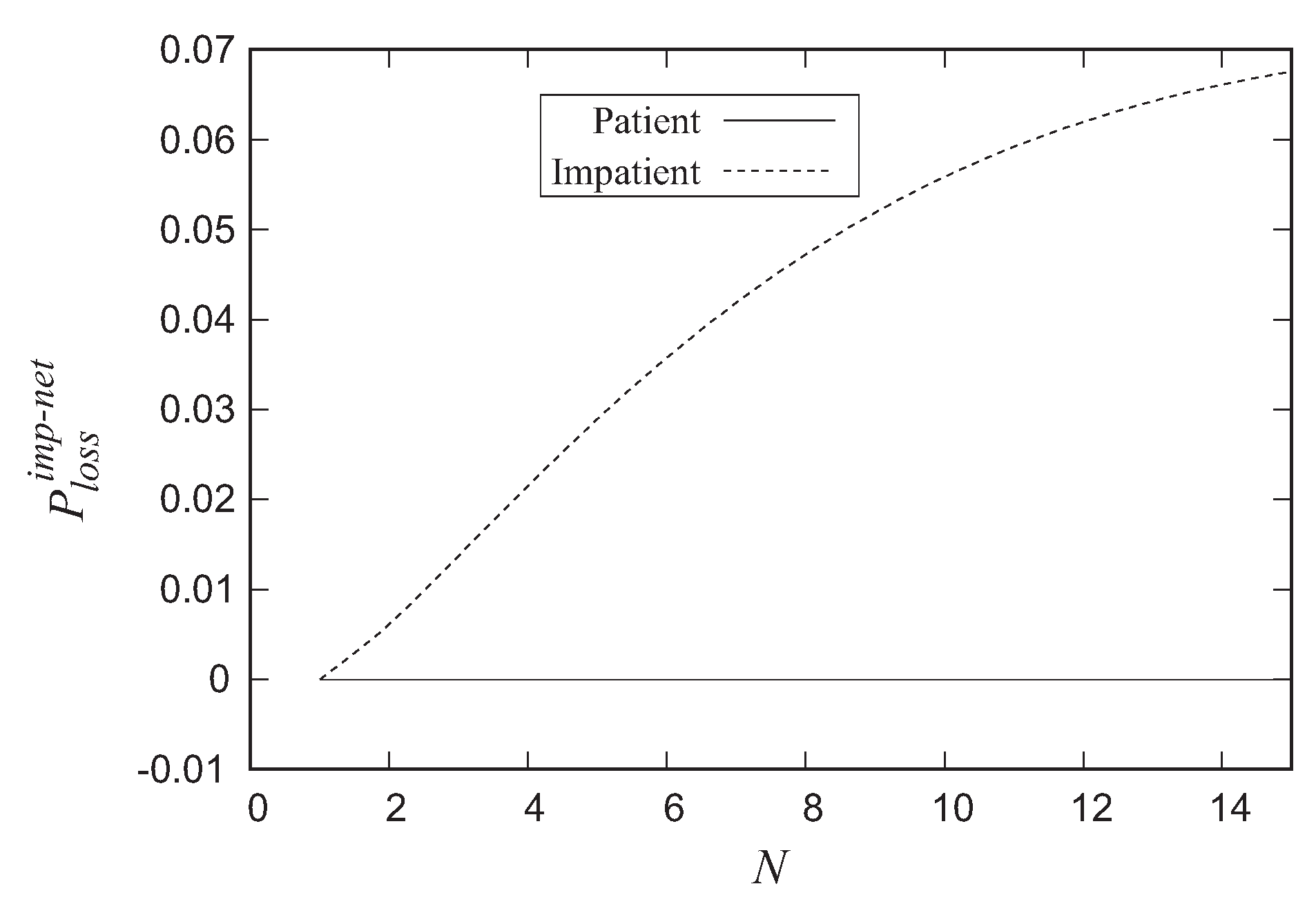
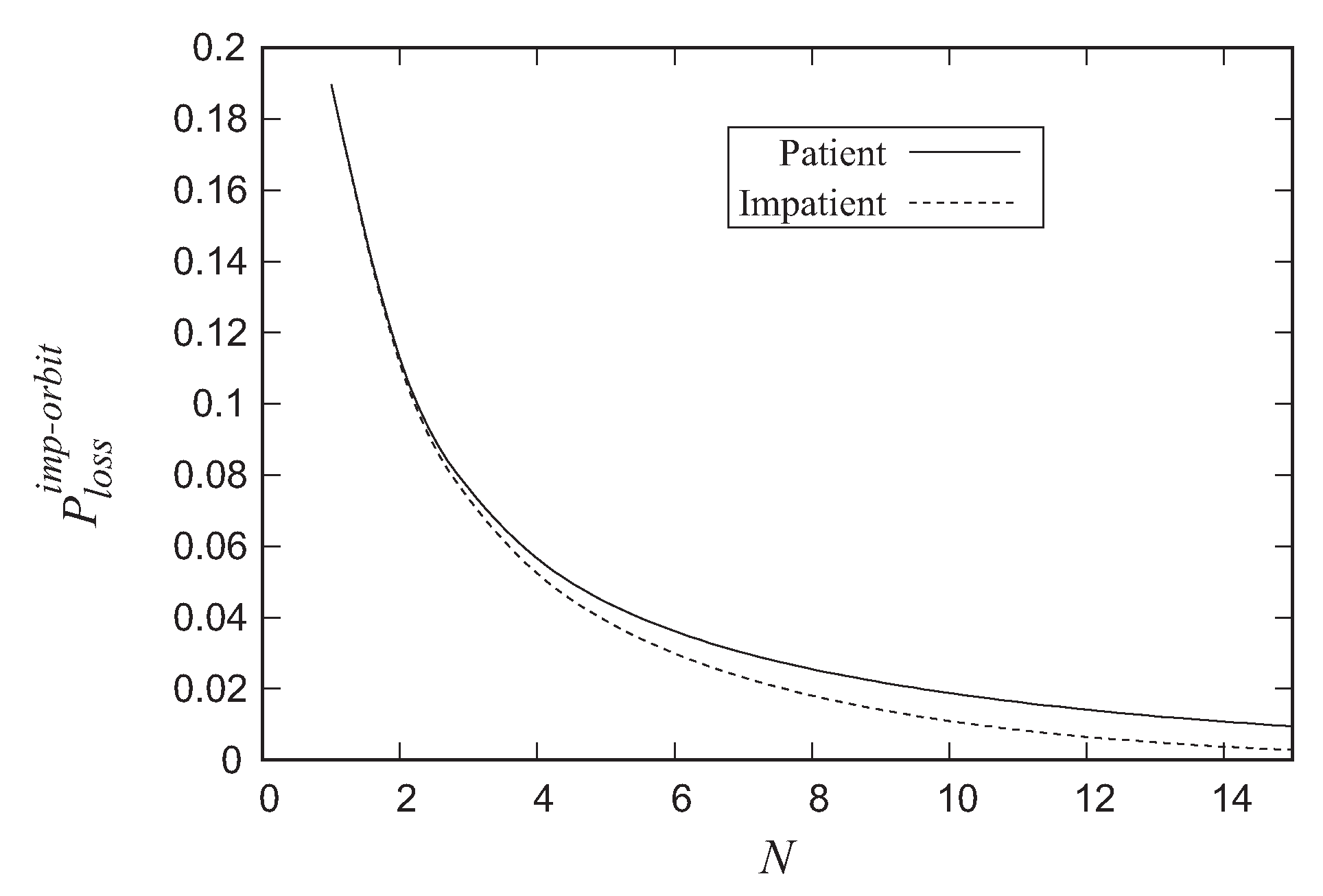
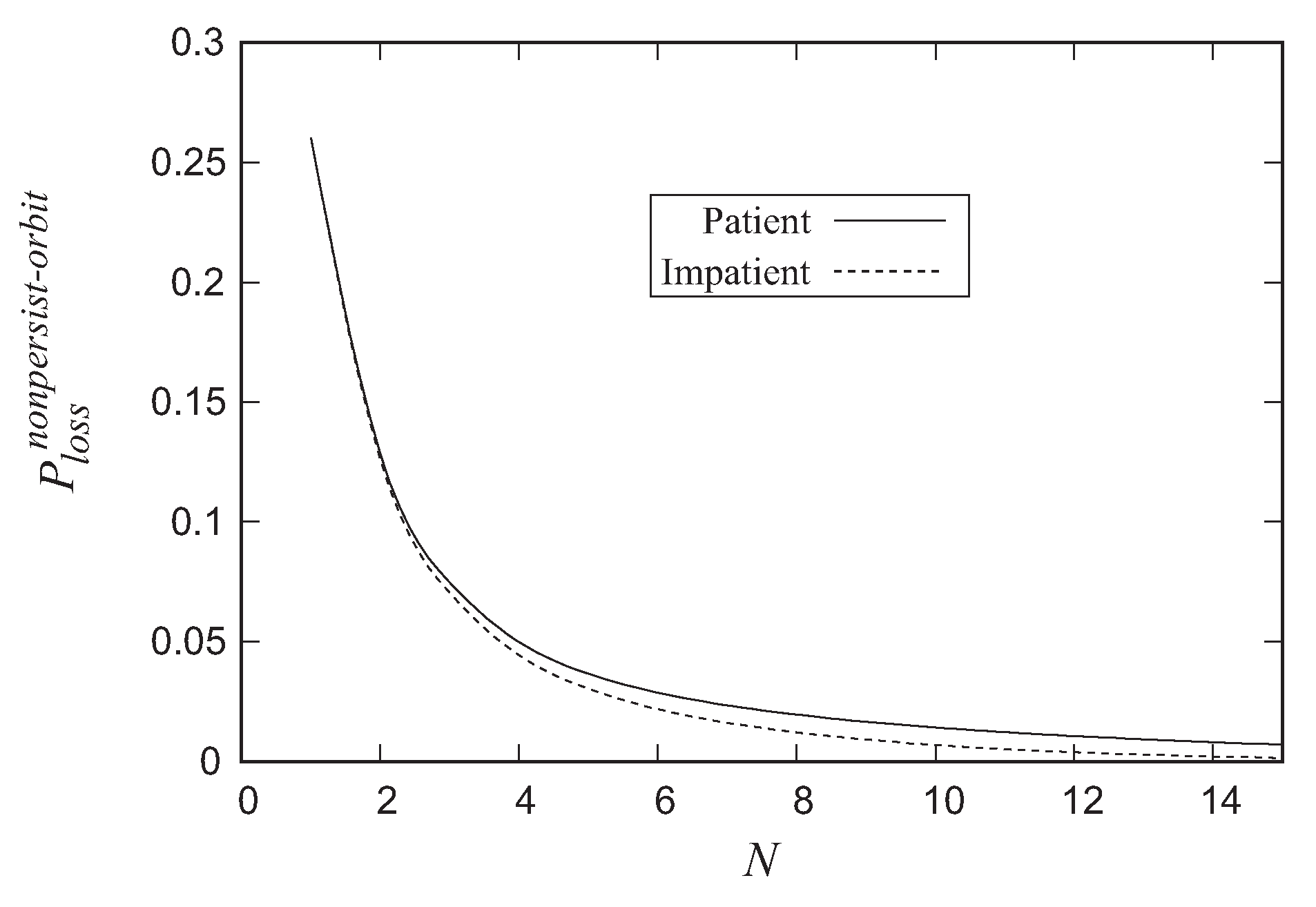
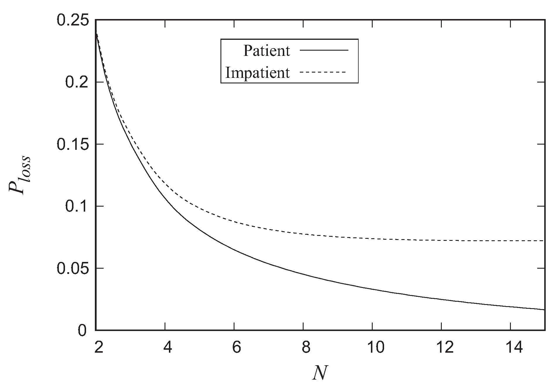
Analogously, Figure 8, Figure 9 and Figure 10 illustrate the dependence on N of the probability of an arbitrary customer loss due to impatience from the orbit $P_{loss}^{imp-orbit}$, the probability of an arbitrary customer loss due to non-persistence from the orbit $P_{loss}^{nonpersist-orbit}$, and the loss probability of an arbitrary customer $P_{loss}$ for the case of the patient and impatient customers in the network.

It can be seen that the impatience in the nodes reduced the probabilities of customers loss from the orbit (due to impatience or non-persistence). However, the total loss probability $P_{loss}$ is essentially higher when the customers in the nodes are impatient. With the growth of N, the difference of values of this probability for the cases of the impatient and patient customers becomes more significant.

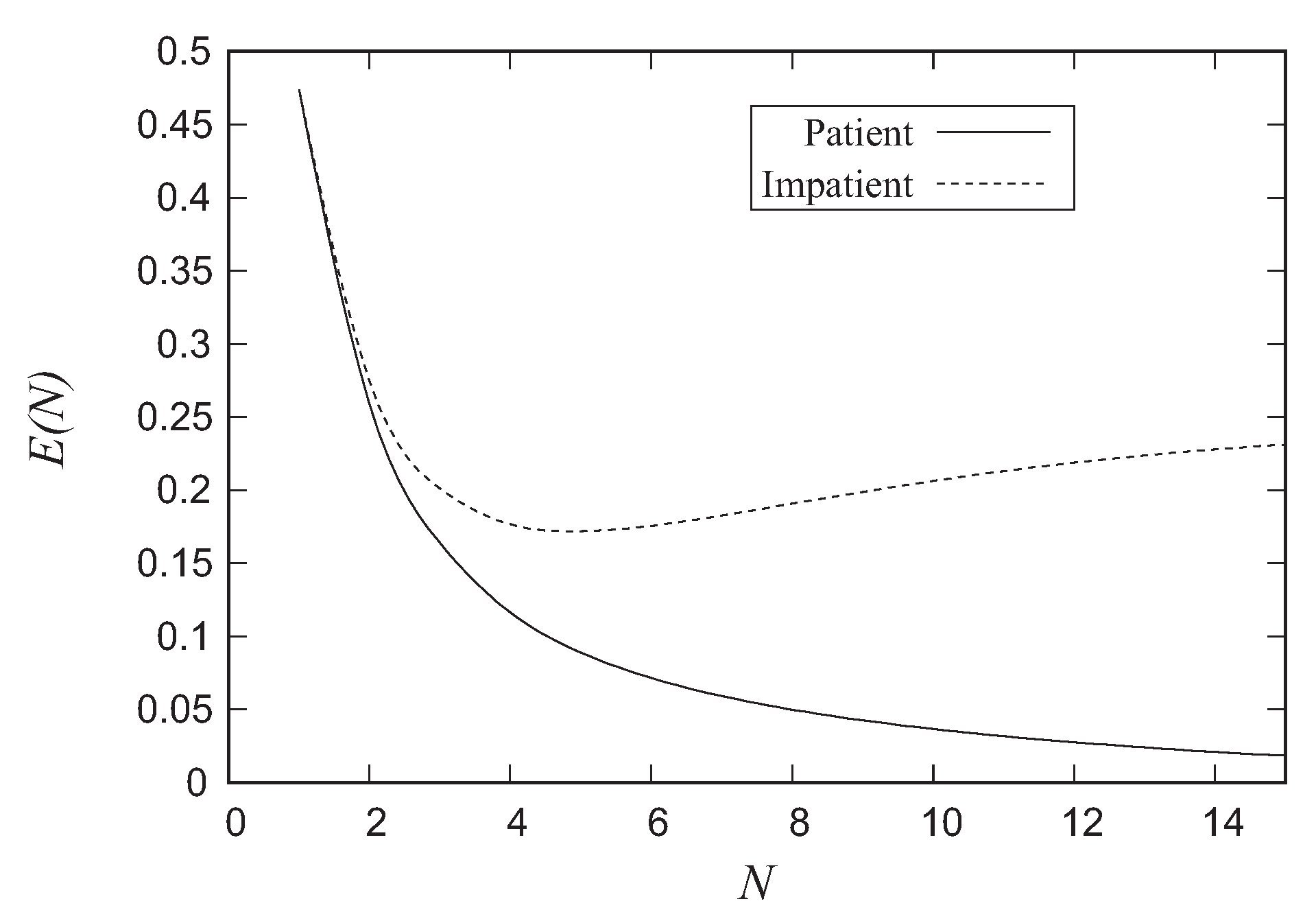
Let us introduce the following economical criterion of the quality of the network operation:

$$E(N)=\widehat{\lambda }(a(P_{loss}^{imp-orbit}+P_{loss}^{nonpersist-orbit})+b{P}_{loss}^{imp-net}),$$

where a is a charge paid for the loss of one customer from the orbit and b is a charge paid for the loss of one customer from the network per unit time. It is evident that the loss of a customer from the network is more painful than the loss of a customer from the orbit because the lost from the network customer possibly have already been serviced in some nodes, that is, the system has spent some resources for providing service to such a customer. Thus, in this example, we assume that $a=1$ and $b=3.$

Figure 11 illustrates the dependence of the economic criterion $E(N)$ on N for the cases of the patient and impatient customers in the network.

The optimal value for the case of patient customers is $E(N)=0.0184$ when $N=15$. This means that in the case of patient customers it is reasonable to accept as many customers as possible. The optimal value for the case of impatient in the network customers is $E(N)=0.171865$ when $N=5.$ Presented in this paper results can be helpful for the optimal choice of the limit N imposed on the number of customers that can be admitted to the network simultaneously.

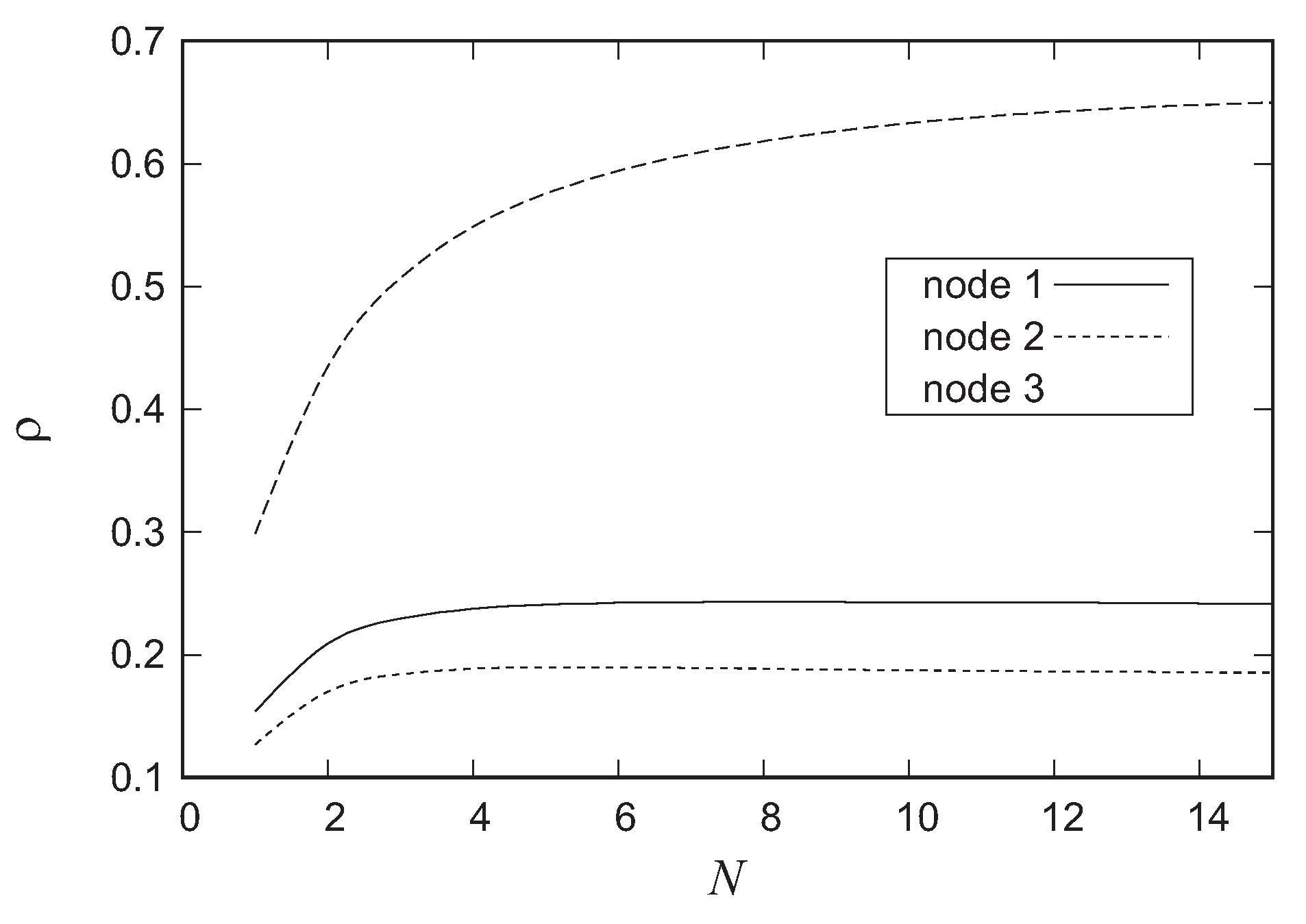
Example 3.

In this experiment, we show how our results can be used for identification of the bottleneck of the network and further improving the performance of the network via the proper upgrade of the bottleneck node. Let us choose the parameters of the network the same as in the previous example in the case of impatient customers. One can see that the loss probability of customers is quite high even for a large value of N ($N=15$). About 7.2% of customers are lost due to different reasons. To understand the reason for such not very good operation of the network, let us compute the average load of each network’s node.

Figure 12 illustrates the dependence of loads of the nodes on the parameter $N.$

As it is seen from this Figure, the load of the third node is much higher than loads of other nodes. Let us make an upgrade of the third node in such a way that after upgrade the service rate in this node increases from 2 to 4 and compute the main performance measures of the network.

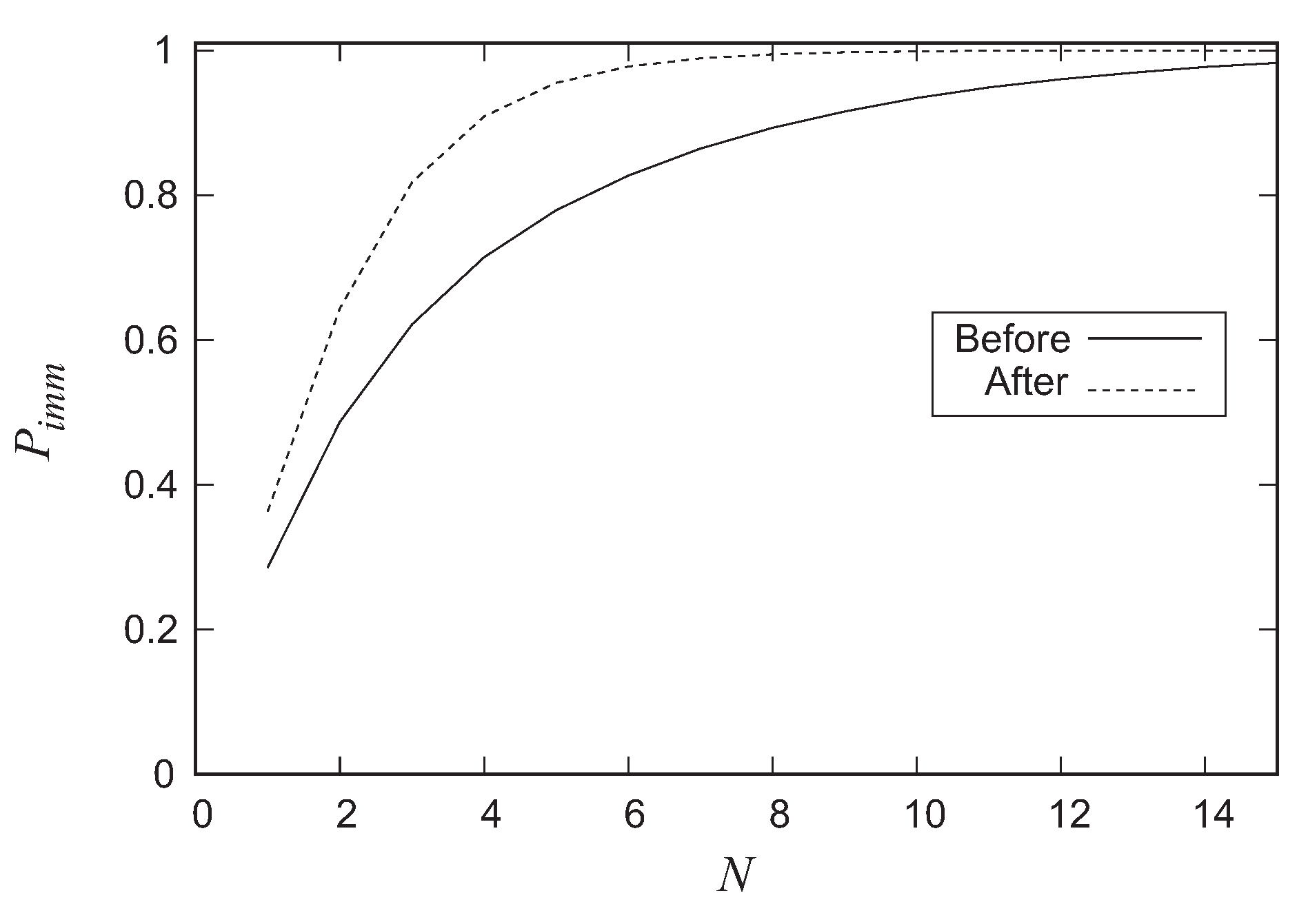
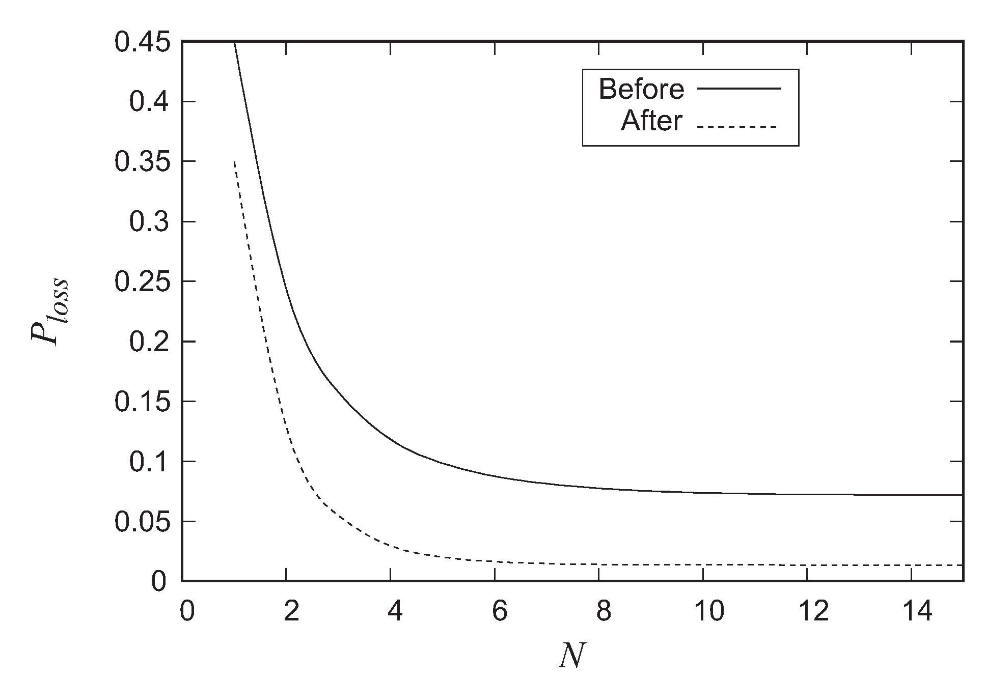
Figure 13 and Figure 14 illustrate the dependence of the probability $P_{imm}$ that an arbitrary customer is admitted to the network immediately upon arrival and the loss probability of an arbitrary customer $P_{loss}$ on the parameter N before and after upgrade.

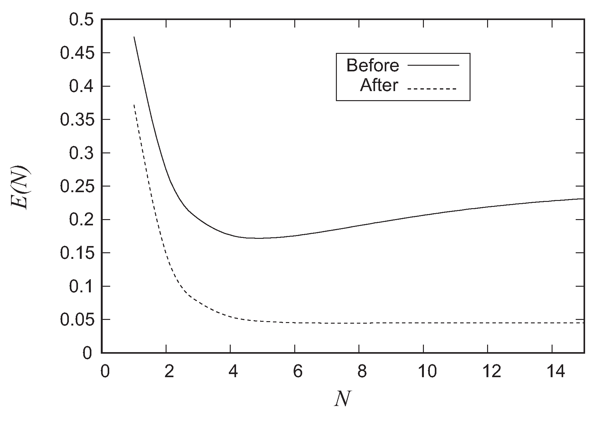
One can see from these Figures that after upgrade the loss probability $P_{loss}$ essentially decreases and the probability $P_{imm}$ of immediate access essentially increases. Figure 15 illustrates the dependence of the economic criterion $E(N)$ on N before and after the upgrade.

The optimal value $E(N)$ after upgrade is $E(N)=0.0448422$ when $N=7$ what is almost four times smaller than the optimal value $E(N)=0.171865$ before the upgrade (that was achieved when $N=5$). Definitely, the increase of the service rate in the third node can cost some money. However, it allows increasing the optimal number of the limit N from 5 to 7 with the essential improvement of the quality of operation of the network.

It is worth to note that the improvement of the quality of operation of the network via the account of loads of the nodes can be achieved also via the modification of the routing of the customers in the node and the choices of the target node by the primary and retrial customers.

6. Conclusions

In this paper, we analyzed a semi-open queuing network with customers retrial. The number of customers in the network must not exceed the fixed threshold (capacity of the network). An arriving primary customer is admitted to the network and starts processing only if the current number of customers in the network is less than the network capacity. Otherwise, the customer moves to the orbit having an infinite capacity and tries to enter the network after random time intervals. The arrivals of primary customers and retrials of customers from the orbit depend on the same underlying process. This allows more adequately model real-world arrival processes than it can be done using known in the literature models of the arrival and retrial processes. Customers are impatient both in the orbit and infinite buffers of the nodes of the network. The behavior of the network is described by a multidimensional Markov chain. The generator of this chain is derived. The problem of computing the stationary state distribution is discussed. The expressions for computing the main performance measures of the network are derived. Numerical results illustrate the importance of the account of the dependency of arrivals of the primary and retrial customers as well as the importance of account of impatience of customers. Possibilities of optimization of the quality of the network operation by means of the optimal choice of the network capacity and identification and elimination of bottlenecks in the network are demonstrated.