On the Rate of Convergence and Limiting Characteristics for a Nonstationary Queueing Model

Abstract

Consideration is given to the nonstationary analogue of $M/M/1$ queueing model in which the service happens only in batches of size 2, with the arrival rate $\lambda \left(t\right)$ and the service rate $\mu \left(t\right)$. One proposes a new and simple method for the study of the queue-length process. The main probability characteristics of the queue-length process are computed. A numerical example is provided.

1. Introduction

Non-stationary Markovian queueing models have been the subject of extensive research for the past few decades. It is well-known that the direct computation of time-dependent characteristics for arbitrary (in)homogeneous continuous-time Markov chains, which show up in the analysis of various queueing models, is a difficult problem. Thus, usually the alternative way is taken: one resorts to different types of approximations. One can find an overview of the approaches for the performance evaluation of time-dependent queueing systems up to 2016 in [1]. The papers [2,3,4] are devoted to the construction of the main performance characteristics and papers [5,6,7,8] deal with the estimation of the convergence rate and approximations. The general framework for the study of time-dependent queueing system systems is described in detail in the recent paper [8]. It consists of several steps, among which the most important one is the estimation of the upper bounds for the rate of convergence to the limiting regime. Having such bound allows one to find (compute) the time instant, say $t^{*}$, starting from which probabilistic properties of $X\left(t\right)$ do not depend on the value of $X\left(0\right)$ (assuming that the process starts at time $t=0$). Thus, for example, if the transition intensities are periodic (say, 1-time-periodic), one can truncate the process on the interval $[t^{*},t^{*}+1]$ and solve the forward Kolmogorov system of differential equations on this interval with $X\left(0\right)=0$. In such a way, one may build approximations for any limiting probability characteristics of $X\left(t\right)$ and estimate stability (perturbation) bounds. For the details regarding the stability bounds, one can refer to [9,10,11,12,13,14,15] and references therein. If the reduced intensity matrix of a Markov chain (see the next section for the definition) is essentially positive, then the approach for the computation of the upper bounds on the rate of convergence $l_1$ metric is available: one may use the method of logarithmic norm of a linear operator function and use the bounds for the Cauchy operator of the (reduced) forward Kolmogorov system (see [6,7]). Note that such bounds may be sharp if the difference between the two initial conditions is nonnegative.

However, the method of the logarithmic norm is not always applicable, i.e., there are Markov chains with such transition intensities, for which it does not yield upper bounds for the rate of convergence. Such a Markov chain is the topic of this paper. Specifically, one considers an inhomogeneous analogue of the classical $M/M/1$ queue, in which the service happens only in batches of size 2. For this queue, we propose the simple new method, based on the direct application of differential inequalities, for the estimation of the queue-size probability characteristics.

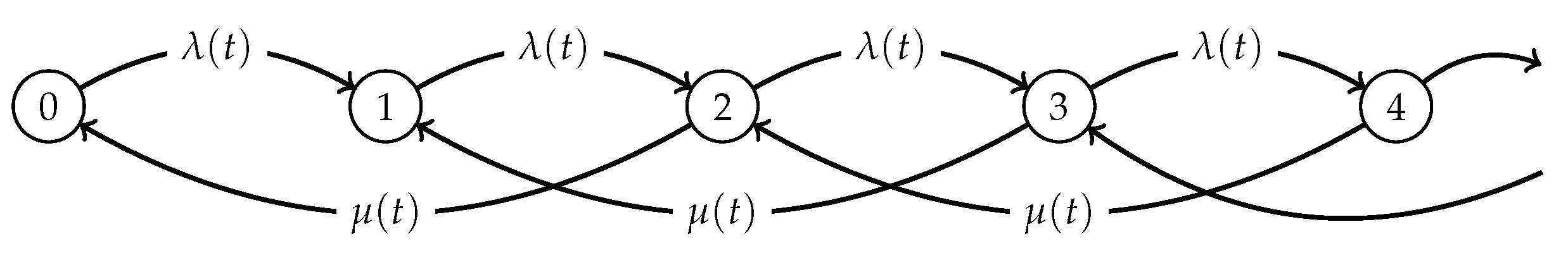
2. Model Description and Basic Transformations

Consideration is given to the Markov chain $X\left(t\right)$ being the queue-length (including a customer in server) at time t in the $M_t/M_t/1$ queuing system with batch service (only). It is assumed that customers enter the system only by one and the arrival intensity does not depend on the number of customers in the system, but depends on time, and is equal to $\lambda \left(t\right)$. Customers can be served only in batches of size 2 and the service intensity does not depend on the number of customers in the system, but depends on time, and is equal to $\mu \left(t\right)$. The transition diagram for $X\left(t\right)$ is given in Figure 1.

Denote by $p_{ij}(s,t)=Pr\left\{X\left(t\right)=j/X\left(s\right)=i\right\}$, $i,j\ge 0,0\le s\le t$ the transition probabilities and by $p_i\left(t\right)=P\left\{X\left(t\right)=i\right\}$—the probability that $X\left(t\right)$ is in state i at time t. Let $\mathbf{p}\left(t\right)={\left(p_0\left(t\right),p_1\left(t\right),\cdots ,p_S\left(t\right)\right)}^T$ be probability distribution vector at instant t. Throughout the paper, it is assumed that

$$\begin{array}{c}\hfill Pr\left(X\left(t+h\right)=j|X\left(t\right)=i\right)=\left\{\begin{array}{cc}\lambda \left(t\right)h+{\alpha }_{ij}\left(t,h\right)& \mathrm{if}j=i+1,i\ge 0,\\ \mu \left(t\right)h+{\alpha }_{ij}\left(t,h\right)& \mathrm{if}j=i-2,i\ge 2,\\ 1-\lambda \left(t\right)h+{\alpha }_i\left(t,h\right)& \mathrm{if}j=i,0\le i\le 1,\\ 1-(\lambda \left(t\right)+\mu \left(t\right))h+{\alpha }_i\left(t,h\right)& \mathrm{if}j=i,i\ge 2,\\ {\alpha }_{ij}\left(t,h\right)& \mathrm{otherwise},\end{array}\right.\end{array}$$

(1)

where all ${\alpha }_{ij}(t,h)$ are $o\left(h\right)$ and ${\alpha }_i(t,h)$ are $o\left(h\right)$ uniformly in i for any $t\ge 0$. In addition, it is assumed that the intensity functions $\lambda \left(t\right)$ and $\mu \left(t\right)$ are nonnegative, continuous and bounded on the interval $[0,\infty )$, $\lambda \left(t\right)+\mu \left(t\right)\le L<\infty$ for any $t\ge 0$. Then, the probabilistic dynamics of the process is represented by the forward Kolmogorov system of differential equations:

$$\frac{d}{dt}\mathbf{p}\left(t\right)=A\left(t\right)\mathbf{p}\left(t\right),$$

(2)

where $A\left(t\right)$ is the transposed intensity matrix of the process, having the following form:

$$A\left(t\right)=\left(\begin{array}{cccccc}-\lambda \left(t\right)& 0& \mu \left(t\right)& 0& 0& \cdots \\ \lambda \left(t\right)& -\lambda \left(t\right)& 0& \mu \left(t\right)& 0& \cdots \\ 0& \lambda \left(t\right)& -\left(\lambda \left(t\right)+\mu \left(t\right)\right)& 0& \mu \left(t\right)& \cdots \\ 0& 0& \lambda \left(t\right)& -\left(\lambda \left(t\right)+\mu \left(t\right)\right)& 0& \cdots \\ \ddots & \ddots & \ddots & \ddots & \ddots & \ddots \\ 0& 0& 0& 0& 0& \cdots \\ \cdots & \cdots & \cdots & \cdots & \cdots & \cdots \end{array}\right).$$

(3)

Throughout the paper, by $\parallel ·\parallel$, we denote the $l_1$-norm, i.e., $\parallel \mathbf{p}\left(t\right)\parallel ={\sum }_{k\ge 0}\left|p_k\left(t\right)\right|$, and $\parallel A\left(t\right)\parallel ={sup}_{j\ge 1}{\sum }_{i\ge 1}\left|a_{ij}\right|$. Let $\Omega$ be a set all stochastic vectors, i.e., $l_1$ vectors with non-negative coordinates and unit norm. Hence, we have $\parallel A\left(t\right)\parallel =2{sup}_{k\ge 1}\left|q_{kk}\left(t\right)\right|\le 2L$ for almost all $t\ge 0$. Hence, the operator function $A\left(t\right)$ from $l_1$ into itself is bounded and continuous for all $t\ge 0$ and thus Label (2) is a differential equation in the space $l_1$ with bounded operator, which has a unique solution for any arbitrary initial condition (see [16]).

The method that is being proposed in this paper relies on the following transformation (referring to [6]) of the intensity matrix $A\left(t\right)$. Since $p_0\left(t\right)=1-{\sum }_{i\ge 1}{p}_i\left(t\right)$ due to the normalization condition, one can rewrite the system (2) as follows:

$$\frac{d}{dt}\mathbf{z}\left(t\right)=B\left(t\right)\mathbf{z}\left(t\right)+\mathbf{f}\left(t\right),$$

(4)

where

$$\mathbf{f}\left(t\right)={\left(\lambda \left(t\right),0,0,\cdots \right)}^T,\mathbf{z}\left(t\right)={\left(p_1\left(t\right),p_2\left(t\right),\cdots \right)}^T,$$

$$B\left(t\right)=\left(\begin{array}{ccccc}-2·\lambda \left(t\right)& -\lambda \left(t\right)& \mu \left(t\right)-\lambda \left(t\right)& -\lambda \left(t\right)& \cdots \\ \lambda \left(t\right)& -\left(\lambda \left(t\right)+\mu \left(t\right)\right)& 0& \mu \left(t\right)& \cdots \\ 0& \lambda \left(t\right)& -\left(\lambda \left(t\right)+\mu \left(t\right)\right)& 0& \cdots \\ \ddots & \ddots & \ddots & \ddots & \ddots \\ 0& 0& 0& 0& \cdots \\ \cdots & \cdots & \cdots & \cdots & \cdots \end{array}\right).$$

(5)

Note that the bounds on the rate of convergence of the solutions of the system of differential equations

$$\frac{d}{dt}\mathbf{y}\left(t\right)=B\left(t\right)\mathbf{y}\left(t\right)$$

(6)

correspond to the same bounds of $X\left(t\right)$.

Denote by T the upper triangular matrix of ones i.e., $t_{ij}=1$ for $j\ge i$ and 0, otherwise. Then,

$$T^{-1}=\left(\begin{array}{ccccc}1& -1& 0& 0& \dots \\ 0& 1& -1& 0& \dots \\ 0& 0& 1& -1& \dots \\ 0& 0& 0& 1& \dots \\ ⋮& ⋮& ⋮& ⋮& \ddots \end{array}\right).$$

Put $\mathbf{u}\left(t\right)=T\mathbf{y}\left(t\right)$. Then, we have

$$\frac{d}{dt}\mathbf{u}\left(t\right)=B^{*}\left(t\right)\mathbf{u}\left(t\right),$$

(7)

where

$$\begin{array}{c}\hfill B^{*}\left(t\right)=\left(\begin{array}{ccccccc}-\lambda \left(t\right)& -\mu \left(t\right)& \mu \left(t\right)& 0& 0& 0& \cdots \\ \lambda \left(t\right)& -\left(\lambda \left(t\right)+\mu \left(t\right)\right)& 0& \mu \left(t\right)& 0& 0& \cdots \\ 0& \lambda \left(t\right)& -\left(\lambda \left(t\right)+\mu \left(t\right)\right)& 0& \mu \left(t\right)& 0& \cdots \\ 0& 0& \lambda \left(t\right)& -\left(\lambda \left(t\right)+\mu \left(t\right)\right)& 0& \mu \left(t\right)& \cdots \\ 0& 0& 0& \lambda \left(t\right)& -\left(\lambda \left(t\right)+\mu \left(t\right)\right)& 0& \cdots \\ \ddots & \ddots & \ddots & \ddots & \ddots & \ddots & \ddots \\ \cdots & \cdots & \cdots & \cdots & \cdots & \cdots & \cdots \end{array}\right).\end{array}$$

Such transformation has been applied in a series of papers for general Markovian queueing models (see, for example, [7]). As it was mentioned above, the analysis of the rate of convergence to the limiting regime (a detailed description of this approach and its generalization can be found, for example, in [8,17,18]) was based on the logarithmic norm of an operator function from $l_1$ to itself, which can be computed by the simple formula:

$$\gamma \left(B\left(t\right)\right)=\underset{j\ge 1}{sup}\left(b_{jj}\left(t\right)+\sum _{i\ge 1,i\ne j}\left|b_{ij}\left(t\right)\right|\right).$$

(8)

For the considered Markov chain $X\left(t\right)$, the method based on the logarithmic norm no longer applied. This is due to the fact that all column sums in $B^{*}\left(t\right)$ are equal to zero. In the next section, one outlines another approach, which is based on the direct applications of the differential inequalities. It was firstly considered for a finite Markovian queueing model in [19].

3. Bounds on the Rate of Convergence

Let $\{d_i,i\ge 0\}$ be a sequence such that ${inf}_{i\ge 0}\left|d_i\right|=d>0$. Denote by $D=diag\left(d_0,d_1,d_2,\dots \right)$ the diagonal matrix. By putting $\mathbf{w}\left(t\right)=D\mathbf{u}\left(t\right)$ from (7), one obtains

$$\frac{d}{dt}\mathbf{w}\left(t\right)=B^{**}\left(t\right)\mathbf{w}\left(t\right),$$

(9)

where the matrix $B^{**}\left(t\right)={\left(b^{**}\left(t\right)\right)}_{i,j=1}^{\infty }=D{B}^{*}\left(t\right)D^{-1}$ has the following form:

$$\begin{array}{c}\hfill B^{**}\left(t\right)=\left(\begin{array}{cccccc}-\lambda \left(t\right)& -\mu \left(t\right)·\frac{d_1}{d_2}& \mu \left(t\right)·\frac{d_1}{d_3}& 0& 0& \cdots \\ \lambda \left(t\right)·\frac{d_2}{d_1}& -\left(\lambda \left(t\right)+\mu \left(t\right)\right)& 0& \mu \left(t\right)·\frac{d_2}{d_4}& 0& \cdots \\ 0& \lambda \left(t\right)·\frac{d_3}{d_2}& -\left(\lambda \left(t\right)+\mu \left(t\right)\right)& 0& \mu \left(t\right)·\frac{d_3}{d_5}& \cdots \\ 0& 0& \lambda \left(t\right)·\frac{d_4}{d_3}& -\left(\lambda \left(t\right)+\mu \left(t\right)\right)& 0& \cdots \\ \ddots & \ddots & \ddots & \ddots & \ddots & \ddots \\ \cdots & \cdots & \cdots & \cdots & \cdots & \cdots \end{array}\right).\end{array}$$

Let $\mathbf{u}\left(t\right)$ be an arbitrary solution of (7). Consider an interval $(t_1,t_2)$ with fixed signs of coordinates of $\mathbf{u}\left(t\right)$. Let now signs of the entries $d_i$ coincide with signs of the corresponding coordinates $u_i\left(t\right)$ of $\mathbf{u}\left(t\right)$. Then, $d_i{u}_i\left(t\right)>0$ for all $i\ge 1$ on the time interval $(t_1,t_2)$ and hence ${\sum }_{k=1}^{\infty }{d}_k{u}_k\left(t\right)=\parallel \mathbf{w}\left(t\right)\parallel$ can be considered as the corresponding norm. Put ${\alpha }_j\left(t\right)=-{\sum }_i{b}_{ij}^{**}\left(t\right)$ and assume that

$${\alpha }_j\left(t\right)\ge {\alpha }_D\left(t\right),j\ge 1.$$

(10)

Consider now the system (9) on the interval $(t_1,t_2)$. Then, the following bound holds:

$$\frac{d}{dt}\parallel \mathbf{w}\left(t\right)\parallel =\frac{d}{dt}\left(\sum _{k\ge 1}{w}_k\left(t\right)\right)=\sum _{j\ge 1}\sum _{i\ge 1}{b}_{ij}^{**}\left(t\right)w_j\left(t\right)\le -{\alpha }_D\left(t\right)\parallel \mathbf{w}\left(t\right)\parallel .$$

(11)

If one puts ${\alpha }^{*}\left(t\right)=inf{\alpha }_D\left(t\right)$, where the infimum is taken over all intervals with different combinations of coordinate signs of the solution, then for any such interval one has in the own corresponding norm, the inequality $\parallel \mathbf{w}\left(t\right)\parallel \le e^{-{\int }_s^t{\alpha }^{*}\left(\tau \right)d\tau }\parallel \mathbf{w}\left(s\right)\parallel$.

Let firstly all coordinates of $\mathbf{u}\left(t\right)$ be positive. Put $d_1=1$, $d_2=1/\delta$, $d_3=\delta$ and $d_{k+1}=\delta d_k$, for $k\ge 3$, where $\delta >1$. Then, one has:

$${\alpha }_1^1\left(t\right)=\lambda \left(t\right)\left(1-{\delta }^{-1}\right),$$

$${\alpha }_2^1\left(t\right)=\mu \left(t\right)\left(1+\delta \right)-\lambda \left(t\right)\left({\delta }^2-1\right),$$

$${\alpha }_3^1\left(t\right)=\mu \left(t\right)\left(1-{\delta }^{-1}\right)-\lambda \left(t\right)\left(\delta -1\right),$$

$${\alpha }_4^1\left(t\right)=\mu \left(t\right)\left(1-{\delta }^{-3}\right)-\lambda \left(t\right)\left(\delta -1\right),$$

$${\alpha }_k^1\left(t\right)=\mu \left(t\right)\left(1-{\delta }^{-2}\right)-\lambda \left(t\right)\left(\delta -1\right),k\ge 5.$$

Therefore, one can take on the corresponding interval ${\alpha }_D^1\left(t\right)={min}_{1\le i\le 4}{\alpha }_i^1\left(t\right)$ and $d^1={inf}_i\left|d_i\right|={\delta }^{-1}$.

Let now $u_1\left(t\right)<0$ and $u_k\left(t\right)>0$ for $k\ge 1$. In this case, we put $d_1=-1$, $d_2=\delta$ and $d_{k+1}=\delta d_k$, for $k\ge 2$, for the same $\delta >1$. Then, one has:

$${\alpha }_1^2\left(t\right)=\lambda \left(t\right)\left(1+\delta \right),$$

$${\alpha }_2^2\left(t\right)=\mu \left(t\right)\left(1-{\delta }^{-1}\right)-\lambda \left(t\right)\left(\delta -1\right),$$

$${\alpha }_3^2\left(t\right)=\mu \left(t\right)\left(1+{\delta }^{-2}\right)-\lambda \left(t\right)\left(\delta -1\right),$$

$${\alpha }_k^2\left(t\right)=\mu \left(t\right)\left(1-{\delta }^{-2}\right)-\lambda \left(t\right)\left(\delta -1\right),k\ge 4.$$

Therefore, one can take on the corresponding interval ${\alpha }_D^2\left(t\right)={min}_{1\le i\le 3}{\alpha }_i^2\left(t\right)$ and $d^2={inf}_i\left|d_i\right|=1$. Moreover, it can be noted that, in any other case, a number of negative elements will be added to the column sums in (10). Hence, all values of ${\alpha }_k\left(t\right)$ in the other situations can only increase, and therefore the corresponding values of ${\alpha }_D\left(t\right)$ for the same $d_k$ will be even greater.

Finally, if one takes ${\alpha }^{*}\left(t\right)=inf{\alpha }_D\left(t\right)$, where the infimum is taken over all intervals with different combinations of coordinate signs of the solution, then the following bounds hold:

$$\begin{array}{c}\hfill {\alpha }^{*}\left(t\right)\ge min\left[\lambda \left(t\right)\left(1-{\delta }^{-1}\right),\mu \left(t\right)\left(1+\delta \right)-\right.\\ \hfill \left.\lambda \left(t\right)\left({\delta }^2-1\right),\mu \left(t\right)\left(1-{\delta }^{-1}\right)-\lambda \left(t\right)\left(\delta -1\right)\right],\end{array}$$

(12)

and the corresponding ‘absolute infimum’

$$d^{*}=min\left(d^1,d^2\right)={\delta }^{-1}.$$

(13)

By applying the comparison of norms, as it was done in [7], one obtains the following theorem.

Theorem 1.

Let

$${\int }_0^{\infty }{\alpha }^{*}\left(t\right)dt=+\infty$$

(14)

for some $\delta >1$. Then, $X\left(t\right)$ is weakly ergodic and the following bounds on the rate of convergence hold:

$$\parallel \mathbf{u}\left(t\right)\parallel \le \delta e^{-{\int }_0^t{\alpha }^{*}\left(\tau \right)d\tau }\parallel \mathbf{w}\left(0\right)\parallel ,$$

(15)

$$\parallel {\mathbf{p}}^{*}\left(t\right)-{\mathbf{p}}^{**}\left(t\right)\parallel \le 4\delta e^{-{\int }_0^t{\alpha }^{*}\left(\tau \right)d\tau }\parallel \mathbf{w}\left(0\right)\parallel ,$$

(16)

for any initial conditions.

Note that the inequality $W={inf}_{k\ge 1}\frac{d_k}{k}>0$ holds for both sequences. It implies an existence of the limiting mean for the process and the corresponding bounds on the rate of convergence (see, for example, [6,7]).

Let the process $X\left(t\right)$ be homogeneous i.e., let $\lambda \left(t\right)=\lambda$ and $\mu \left(t\right)=\mu$ be positive numbers. Then, (14) is equivalent to ${\alpha }^{*}>0$ and this is equivalent to $0<\lambda <\mu$. Put $\delta =\sqrt{\frac{\mu }{\lambda }}$. Hence,

$${\alpha }_0^{*}=min\left[{\left(\sqrt{\mu }-\sqrt{\lambda }\right)}^2,\lambda \left(1-\sqrt{\frac{\lambda }{\mu }}\right)\right],$$

(17)

and the following is the corollary to Theorem 1.

Corollary 1.

Let $X\left(t\right)$ be the queue-length process in $M/M/1$ queue with service in batches of size 2. Let $0<\lambda <\mu$. Then, $X\left(t\right)$ is ergodic and the following bounds hold:

$$\parallel \mathbf{u}\left(t\right)\parallel \le \delta e^{-{\alpha }_0^{*}t}\parallel \mathbf{w}\left(0\right)\parallel ,$$

(18)

and

$$\parallel {\mathbf{p}}^{*}\left(t\right)-\pi \parallel \le 4\delta e^{-{\alpha }^{*}t}\parallel \mathbf{w}\left(0\right)\parallel ,$$

(19)

for any initial condition $X\left(0\right)$.

Note that the inequality $W={inf}_{k\ge 1}\frac{d_k}{k}>0$ implies an existence of the constant limiting mean for the process and the corresponding bounds on the rate of convergence.

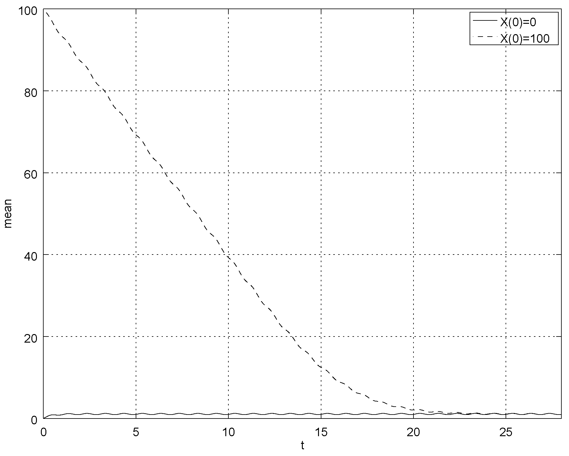
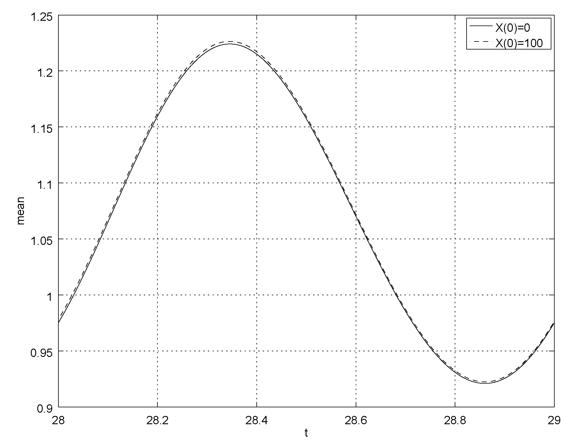
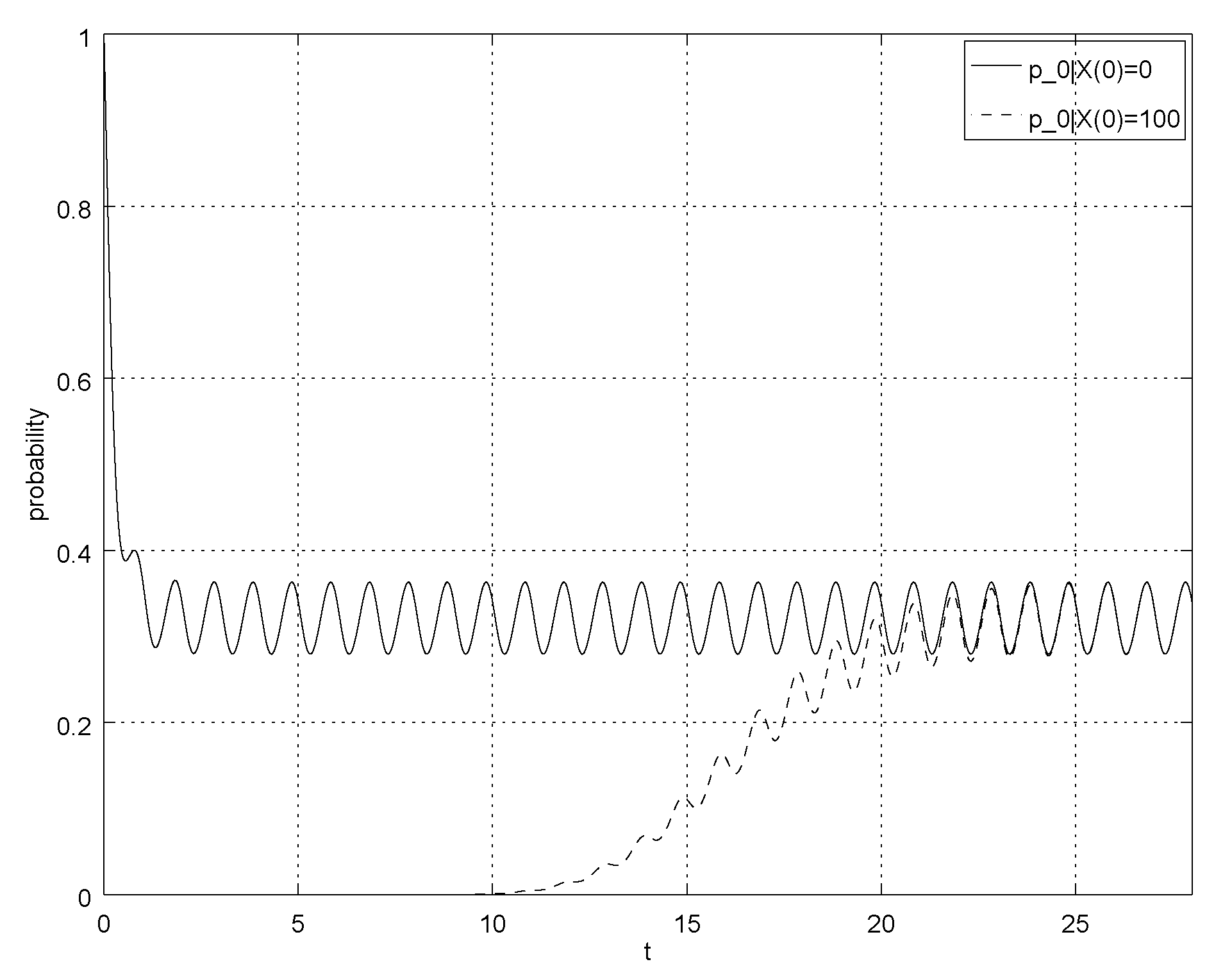
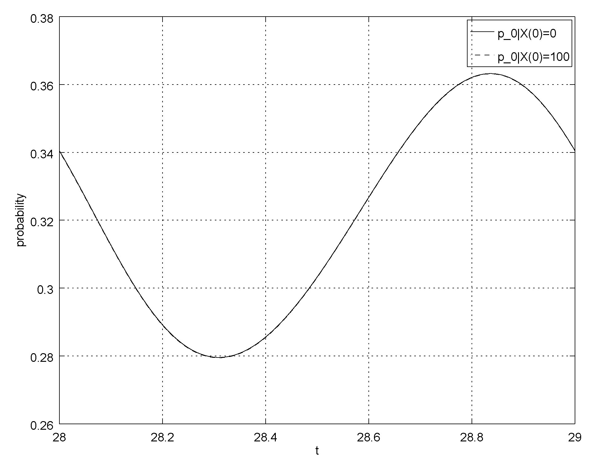
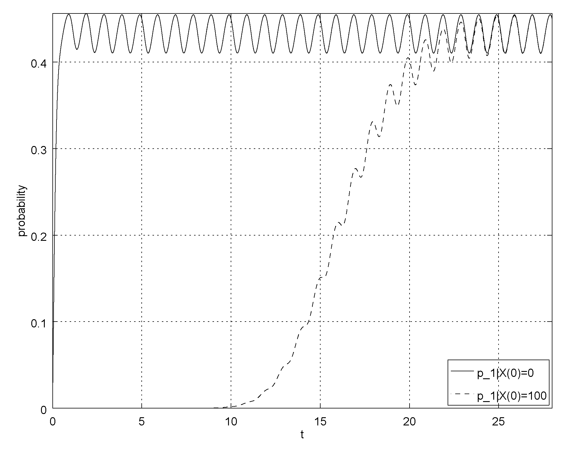
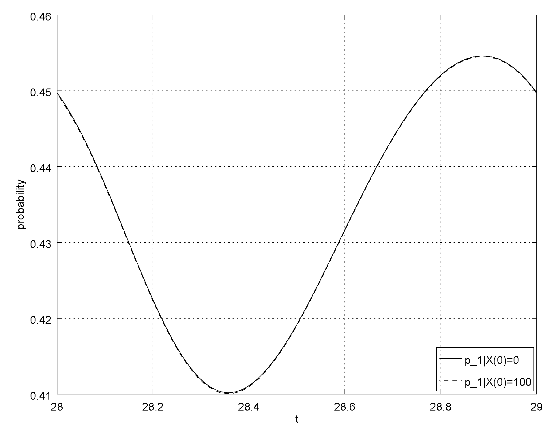
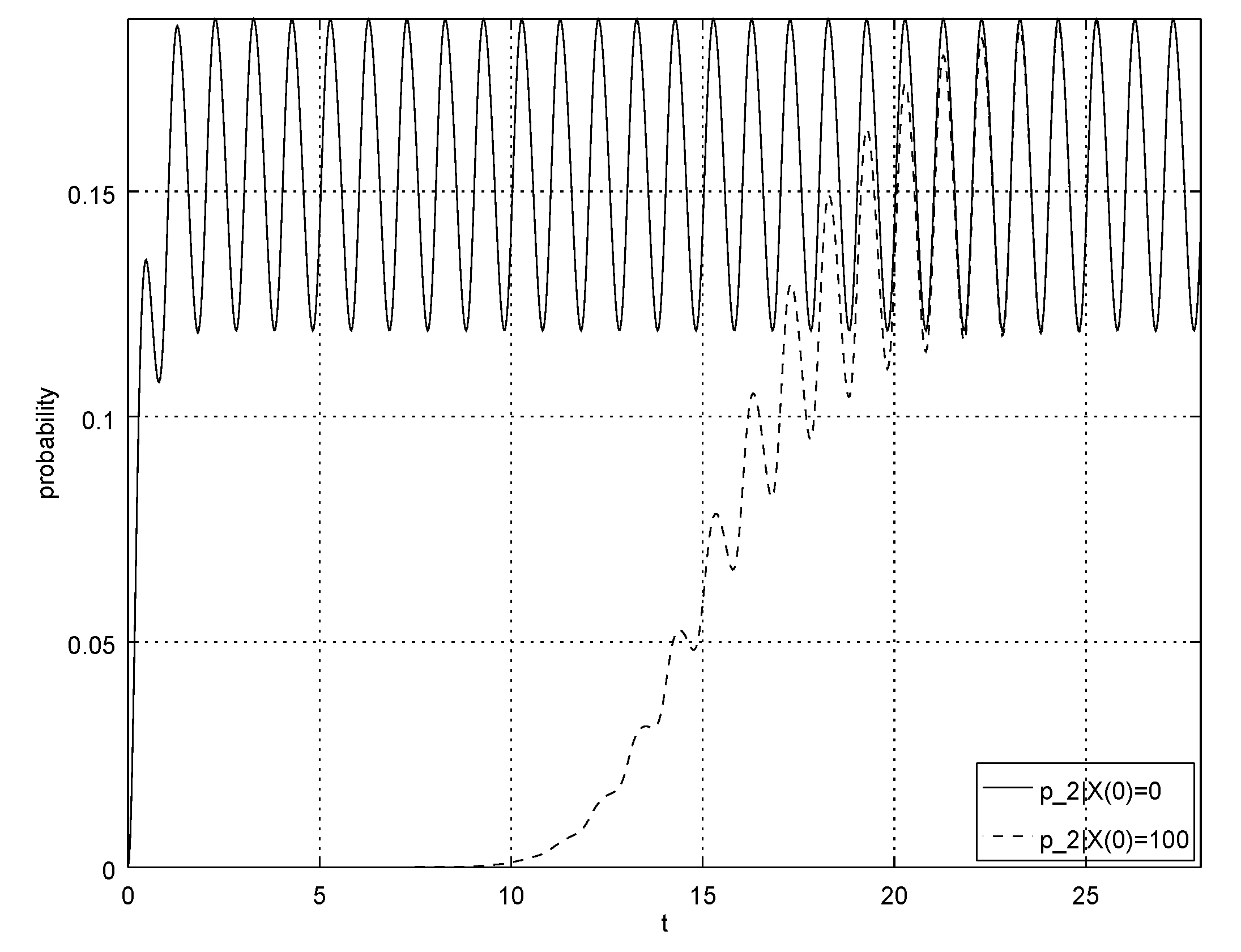
4. Numerical Example

There exists a number of investigations of queueing models with service in batches (or group services) (see, for example, [20,21]). Consider one example of such a queueing model with periodic arrival and service rates. We will be interested in the following quantities: $p_i\left(t\right)$ the probability that the total number of customers in the system at time t is i and the mean number $E(t,k)=E\left(X\right(t\left)\right|X\left(0\right)=k)$ of customers in the system at time t, provided that initially (at instant $t=0$), there were k customers in the system.

Let $\lambda \left(t\right)=2+sin2\pi t$ and $\mu \left(t\right)=4-cos2\pi t$. Put $\delta =\frac{11}{10}$. Then, ${\int }_0^1{\alpha }^{*}\left(t\right)dt\ge \frac{1}{22}>0$ and the assumptions of Theorem 1 are fulfilled. Hence, $X\left(t\right)$ is exponentially weakly ergodic ( i.e., ${lim}_{t\to \infty }\parallel {\mathbf{p}}^{*}\left(t\right)-{\mathbf{p}}^{**}\left(t\right)\parallel \to 0$ for any initial conditions ${\mathbf{p}}^{*}\left(0\right)$ and ${\mathbf{p}}^{**}\left(0\right)$, where ${\mathbf{p}}^{*}\left(t\right)$ and ${\mathbf{p}}^{**}\left(t\right)$ are the solutions of (2)) and has the 1-periodic limiting mean (A Markov chain has the limiting mean $m\left(t\right)$, if ${lim}_{t\to \infty }\left(m\left(t\right)-E(t,k)\right)=0$ for any k.) $m\left(t\right)$. Now, applying the known truncation technique (See the detailed discussion and bounds in [22]), one can compute all probability characteristics of the queue-length process $X\left(t\right)$. The corresponding graphs are shown in Figure 2, Figure 3, Figure 4, Figure 5, Figure 6, Figure 7, Figure 8 and Figure 9. To ensure that the truncation error is less than ${10}^{-3}$, one can truncate the process $X\left(t\right)$ at the level $N=100$. Then, one can compute any probability characteristic using the “extreme” initial conditions $X\left(0\right)=0$ and $X\left(0\right)=N=100$. Inequality (16) gives the corresponding (very rough) upper bounds on the rate of convergence for the state probabilities and for the mean number of customers in the system. Therefore, one can compute all characteristics on the intervals $[0,t^{*}]$ and $[t^{*},t^{*}+1]$, and obtain the limiting state probabilities and the limiting mean with error less $2\times {10}^{-3}$. In Figure 2, Figure 3, Figure 4, Figure 5, Figure 6, Figure 7, Figure 8 and Figure 9 below, it can be seen that in fact it suffices to set $t^{*}=28$. Figure 2, Figure 4, Figure 6 and Figure 8 show the mean number of customers in the system and the probabilities $p_0\left(t\right)$, $p_1\left(t\right)$ and $p_2\left(t\right)$ converge to their limiting values. One can explicitly see how they approach the time $t^{*}$, starting from which the characteristics do not longer depend on the initial conditions. Other figures show their approximate limiting values.

5. Conclusions

In the paper, some estimates of the rate of convergence and the corresponding approach were discussed for an inhomogeneous countable state continuous-time Markov chain. This chain is considered as the queue-length process of a simple nonstationary model of a queue with single arrivals and batch service (only in batches of size 2). The applied approach allows for studying new classes of the continuous-time Markov chain such that the corresponding reduced intensity matrix is not essentially nonnegative.

References

1. Schwarz, J.A.; Selinka, G.; Stolletz, R. Performance analysis of time-dependent queueing systems: Survey and classification. Omega 2016, 63, 170–189. [Google Scholar] [CrossRef] [Green Version]
2. Di Crescenzo, A.; Giorno, V.; Krishna Kumar, B.; Nobile, A.G. A Time-Non-Homogeneous Double-Ended Queue with Failures and Repairs and Its Continuous Approximation. Mathematics 2018, 6, 81. [Google Scholar] [CrossRef]
3. Giorno, V.; Nobile, A.G.; Spina, S. On some time non-homogeneous queueing systems with catastrophes. Appl. Math. Comp. 2014, 245, 220–234. [Google Scholar] [CrossRef]
4. Ammar, S.I.; Alharbi, Y.F. Time-dependent analysis for a two-processor heterogeneous system with time-varying arrival and service rates. Appl. Math. Model. 2018, 54, 743–751. [Google Scholar] [CrossRef]
5. Meyn, S.P.; Tweedie, R.L. Stability of Markovian processes III: Foster- Lyapunov criteria for continuous time processes. Adv. Appl. Probab. 1993, 25, 518–548. [Google Scholar] [CrossRef]
6. Zeifman, A.; Leorato, S.; Orsingher, E.; Satin Ya Shilova, G. Some universal limits for nonhomogeneous birth and death processes. Queueing Syst. 2006, 52, 139–151. [Google Scholar] [CrossRef] [Green Version]
7. Zeifman, A.; Razumchik, R.; Satin, Y.; Kiseleva, K.; Korotysheva, A.; Korolev, V. Bounds on the Rate of Convergence for One Class of Inhomogeneous Markovian Queueing Models with Possible Batch Arrivals and Services. Int. J. Appl. Math. Comp. Sci. 2018, 28, 141–154. [Google Scholar] [CrossRef]
8. Zeifman, A.; Satin, Y.; Kiseleva, K.; Korolev, V.; Panfilova, T. On limiting characteristics for a non-stationary two-processor heterogeneous system. Appl. Math. Comput. 2019, 351, 48–65. [Google Scholar] [CrossRef] [Green Version]
9. Kartashov, N.V. Criteria for uniform ergodicity and strong stability of Markov chains with a common phase space. Theory Probab. Appl. 1985, 30, 71–89. [Google Scholar]
10. Liu, Y. Perturbation bounds for the stationary distributions of Markov chains. SIAM J. Matrix Anal. Appl. 2012, 33, 1057–1074. [Google Scholar] [CrossRef]
11. Mitrophanov, A.Y. Stability and exponential convergence of continuous-time Markov chains. J. Appl. Probab. 2003, 40, 970–979. [Google Scholar] [CrossRef]
12. Mitrophanov, A.Y. The spectral gap and perturbation bounds for reversible continuous-time Markov chains. J. Appl. Probab. 2004, 41, 1219–1222. [Google Scholar] [CrossRef] [Green Version]
13. Zeifman, A.I.; Korolev, V.Y. On perturbation bounds for continuous-time Markov chains. Stat. Probab. Lett. 2014, 88, 66–72. [Google Scholar] [CrossRef]
14. Mitrophanov, A.Y. Connection between the Rate of Convergence to Stationarity and Stability to Perturbations for Stochastic and Deterministic Systems. In Proceedings of the 38th International Conference Dynamics Days Europe (DDE 2018), Loughborough, UK, 3–7 September 2018; Available online: http://alexmitr.com/talk_DDE2018_Mitrophanov_FIN_post_sm.pdf (accessed on 29 June 2019).
15. Rudolf, D.; Schweizer, N. Perturbation theory for Markov chains via Wasserstein distance. Bernoulli 2018, 24, 2610–2639. [Google Scholar] [CrossRef] [Green Version]
16. Daleckij, J.L.; Krein, M.G. Stability of Solutions of Differential Equations in Banach Space; American Mathematical Society: Providence, RI, USA, 2002; Volume 43. [Google Scholar]
17. Sinitcina, A.; Satin, Y.; Zeifman, A.; Shilova, G.; Sipin, A.; Kiseleva, K.; Panfilova, T.; Kryukova, A.; Gudkova, I.; Fokicheva, E. On the Bounds for a Two-Dimensional Birth-Death Process with Catastrophes. Mathematics 2018, 6, 80. [Google Scholar] [CrossRef]
18. Zeifman, A.; Satin, Y.; Kiseleva, K.; Korolev, V. On the Rate of Convergence for a Characteristic of Multidimensional Birth-Death Process. Mathematics 2019, 7, 477. [Google Scholar] [CrossRef]
19. Zeifman, A.; Satin, Y.; Kiseleva, K.; Kryukova, A. Applications of Differential Inequalities to Bounding the Rate of Convergence for Continuous-time Markov Chains. AIP Conf. Proc. 2019, 2116, 090009. [Google Scholar]
20. Brugno, A.; D’Apice, C.; Dudin, A.; Manzo, R. Analysis of an MAP/PH/1 queue with flexible group service. Int. J. Appl. Math. Comp. Sci. 2017, 27, 119–131. [Google Scholar] [CrossRef]
21. Lee, H.W.; Baek, J.W.; Jeon, J. Analysis of the MX/G/1 queue under D-policy. Stoch. Anal. Appl. 2005, 23, 785–808. [Google Scholar] [CrossRef]
22. Zeifman, A.; Satin Ya Korolev, V.; Shorgin, S. On truncations for weakly ergodic inhomogeneous birth and death processes. Int. J. Appl. Math. Comp. Sci. 2014, 24, 503–518. [Google Scholar] [CrossRef] [Green Version]
Figure 1. Transition diagram for the Markov chain X ( t ) .
Mathematics 07 00678 g001
Figure 2. Example. The mean E ( t , 0 ) and E ( t , 100 ) for t [ 0 , 28 ] , this figure shows the rate of convergence.
Mathematics 07 00678 g002
Figure 3. Example. The mean E ( t , 0 ) and E ( t , 100 ) for t [ 28 , 29 ] , this figure shows approximation of the limiting mean.
Mathematics 07 00678 g003
Figure 4. Example. Probability of the empty queue p 0 ( t ) for t [ 0 , 28 ] and initial conditions X ( 0 ) = 0 and X ( 0 ) = 100 , this figure shows the rate of convergence.
Mathematics 07 00678 g004
Figure 5. Example. Probability of the empty queue p 0 ( t ) for t [ 28 , 29 ] and initial conditions X ( 0 ) = 0 and X ( 0 ) = 100 , this figure shows approximation of the limiting probability p 0 ( t ) .
Mathematics 07 00678 g005
Figure 6. Example. Probability p 1 ( t ) for t [ 0 , 28 ] and initial conditions X ( 0 ) = 0 and X ( 0 ) = 100 , this figure shows the rate of convergence.
Mathematics 07 00678 g006
Figure 7. Example. Probability p 1 ( t ) for t [ 28 , 29 ] and initial conditions X ( 0 ) = 0 and X ( 0 ) = 100 , this figure shows approximation of the limiting probability p 1 ( t ) .
Mathematics 07 00678 g007
Figure 8. Example. Probability p 2 ( t ) for t [ 0 , 28 ] and initial conditions X ( 0 ) = 0 and X ( 0 ) = 100 , this figure shows the rate of convergence.
Mathematics 07 00678 g008
Figure 9. Example. Probability p 2 ( t ) for t [ 28 , 29 ] and initial conditions X ( 0 ) = 0 and X ( 0 ) = 100 , this figure shows approximation of the limiting probability p 2 ( t ) .
Mathematics 07 00678 g009