Evolutionary Game Analysis of the Effects of Problem Size and the Problem Proposing Mechanism on the Problem Processing Mechanism in a New Main Manufacturer–Supplier Collaborative System

Abstract

This paper analyzed the effects of the problem size and the problem proposing mechanism on the decision-making processes, for the manufacturer and the supplier, regarding processing a problem in a new main manufacturer–supplier collaborative system using evolutionary game theory. Unpredicted problems may arise in the process of collaborative research and development (R&D) of complex products, like big passenger aircrafts, without any relative advanced contract, and either player will take risks to announce it. In addition to the factors of traditional cost and income, we take another two factors (i.e., the problem size and the problem proposing mechanism) into account in the examination of the problem processing mechanism. With evolutionary game theory applied, we can obtain the stable decision-making states of both players and how these two factors affect the problem processing mechanism. From the result, we find that the problem size has little effect on the two players’ decisions, while the problem processing mechanism has an impact when the experiences or the capacities of the manufacturer and the supplier are unbalanced. This paper contributes to manufacturer and supplier in a newly-established collaborative system to consider how to behave when unpredicted problems come.

1. Introduction

Recently, two air crashes involving Boeing 737 MAX 8 in October, 2018 and March, 2019 have attracted our attention once again to the research and development (R&D) of complex products and their special production mode. Complex product refers to a kind of large-scale product or system with a complex product structure, high price, high engineering technology content, and high assembling of parts [1], such as mobile phones, aircraft, large ships, satellites, launch vehicles, and so on. These kinds of products have to be assembled with a wide variety of subsystems, components, and parts, the production process of which is extremely complex and difficult to operate [2,3,4]. Particularly, due to the personalized and professional needs of customers, complex products are usually produced in single or small batches, which is different from the mass production system of ordinary products. A principle called “main manufacturer–supplier” mode, which is abbreviated as M-S, has been widely used in the R&D of numerous complex products, such as big passenger aircraft [5]. With regards to complex products’ characteristics, like complex product structure, complex production technology, complex manufacturing activities, and complex management process, M-S mode requires that complex products must be manufactured through collaborative production of multiple enterprises [6,7,8]. In M-S mode, the manufacturer and its suppliers have to work cooperatively in the R&D of the products, work together when problems arise in the production process, and share the risk [9].

With the progress of material civilization, the demand of complex products is increasing, and the demand orientation is increasingly diversified. Due to technological progress, competition among enterprises, and diversification of development directions of enterprises, the manufacturer is not satisfied with establishing a long-term partnership with only one supplier. In order to produce diversified products to meet the needs of different customers, they began to establish cooperative relationships with substitutable suppliers, such as Boeing’s contract cancellation with GKN, the engine thrust device supplier of 737MAX aircraft, and new relationship establishment with CFM International in 2015, to increase production. Moreover, as a result of the slow transformation for some old enterprises, like MOTOROLA, who was once a highly qualified mobile phone manufacturer, or the need for national strategic development, many new manufacturers and suppliers have emerged as the times require, such as COMAC, China’s manufacturer of big passenger aircraft. Lots of new relationships between manufacturers and suppliers in the R&D of some complex products are established thereby [10].

In these new relationships, some unpredicted problems during the R&D process arise and no relative contract are signed beforehand. For example, there have been frequent controversies over the security problems of C919, the first big passenger aircraft product by COMAC. Many of the problems were unpredicted in advance by the young manufacturer COMAC and its suppliers before they signed the collaboration, even though some of the suppliers are experienced. Due to the complexity of complex products, the problems arising in the R&D of complex products are more complicated and diverse than those of ordinary products [9,10,11,12]. Thus, the probability of the unpredicted problems is much higher. The manufacturers and the suppliers would have to bear much more risk during the collaboration in the R&D of complex products than that of ordinary products. For example, the grounding of 737MAX project has brought troubles to Boeing and its suppliers. The loss is considerable, but they still cannot find a way to solve the existing problems and some other unpredicted problem. Therefore, it is important to conduct research on the unpredicted problems in the R&D of complex products. But it will be difficult to quantitatively characterize the unpredicted problems and the way the manufacturer and the supplier behave to the problems.

In our work, we consider that the size of the unpredicted problems in the R&D process of complex products can be quantified in terms of the evaluation of risks [13,14,15] that the manufacturer and the supplier would bear in common. Here, we consider the risks as financial risks brought by the issues like schedule delay. Different from ordinary products, there are many differences in various risk levels for the manufacturer and supplier brought by different sizes of problems, such as difficulty levels of correcting. For example, in the R&D of aircraft, problems brought by the adjustment of the windows’ sizes are much smaller than the problems brought by the adjustment of the engine’s size. Thus, the problem size may affect the behaviors of the manufacturer and the supplier on the unpredicted problem.

Besides, the one who proposes the problem in the R&D of complex products would take more risk to pay it off [16] in the process of dealing with the problem collaboratively. Plus, the proposer of a problem refers to the one who observes a problem, comes up with the problem, and is primarily responsible for proposing the solution of the problem. Therefore, as our work focus on the behaviors of the manufacturer and the supplier processing the problem, we would also consider the effects of the behaviors of proposing the problem and the relationship between these two kinds of behaviors in our paper.

We consider that the cognitive and computational abilities of the manufacturer and supplier in the newly-established R&D collaborative relationship of a complex product are limited. Given these decision-makers have bounded rationalities in real life, we make an attempt at evolutionary game theory [17] to explore how the following factors affect both the manufacturer and the supplier processing the problem: (1) the problem size, and (2) whether or not to take the risk of proposing the problem. It would be hard to characterize the unpredicted problem processing mechanism in a newly-established R&D collaborative system in our model, but our work is meaningful. The analysis results on how the factors affect the decision behaviors of the manufacturer and the supplier when processing unpredicted problems can better inform the two players in a newly-established system of how to reduce the risk. Cost can be arranged in a reasonable range when facing various problem sizes and skills can be grasped easily when proposing a problem to avoid waste.

The remaining three sections are organized as follows. Section 2 tracks the relevant theoretical bases and literature bases, details our modeling assumptions, and establishes the game payoff model for the manufacturer and supplier. Section 3 analyses its equilibrium states, as well as the relative existing conditions, and identifies the impacts of the problem size and the problem proposing mechanism. Section 4 offers discussions on the theoretical and practical significance of the paper, and suggestions for future research.

2. Methods

2.1. Theoretical Backgrounds and Assumptions

In order to address the problem posed in Section 1, we will firstly review some relative theoretical backgrounds and propose the assumptions in this section accordingly.

2.1.1. Main Manufacturer–Supplier Collaborative Mode

In 1969, the proposition of the functional capability of integrated circuits at decreasing cost, which is called large-scale integration (LSI) [18], is dedicated to some possible standardization on the systems manufacturer being not “locked in” to one supplier. This is the earliest research about M-S mode to the best of our knowledge. Some early research have been done about the M-S mode’s application in complex products, such as the pilot case study considering suppliers of parts and small components and a major manufacturer of automotive components [2]; the stock turnover data analysis and the manufacturing performances comparison on the motor industry between Japanese and the Western countries with the M-S mode considered [3]; the effective investment option exploration regarding the lead-time variance reduction and a long-term partnership establishment with suppliers for Japanese manufacturers [4]; and so on. Besides, prior research have emphasized the importance of M-S mode in the R&D of complex products. The importance of developing a collaboration relationship between the manufacturer and the supplier is examined and emphasized considering the combination of the manufacturer’s rush order contract and the supplier’s advance order discount contract to avoid the inventory risk [9], global manufacturing networks alignment as the guideline to open logistics performance, and cost potentials [11], the functions and operations of the manufacturer and the supplier to secure preparations for production ramp-up in a new product R&D project [10], and stochastic demand during a selling season and asymmetric cost information of the supplier [12].

In the M-S production system, the manufacturer plays a role as production organizer and system integrator, mainly working on construction of an efficient supply chain; design of overall product, formulation, and supervision on the required quality of supplier; and delivery of final products [19,20,21]. The supplier needs to cooperate with the manufacturer to complete product assembly [22,23,24].

Both the manufacturer and the supplier have to share the responsibility for any problems and risks in the production process and even after the delivery of the product. In order to ensure the quality of products and avoid the loss caused by risks, such as brand reputation damage, market share shrinkage, and so on, the manufacturer and supplier need to invest part of their resources to ensure the quality of products [25,26,27,28]. Our work will be based on the complete understanding [29] of manufacturer and supplier sharing risks and rewards in an effective collaboration with key strategic and operational results. As long as there are no problems, or problems in the production process are reasonably solved, according to the contract, both players will share the benefits of the product. Thus, the following assumption is proposed:

A1. We consider a two-echelon supply chain and a collaborative R&D mechanism with one upstream supplier and one downstream manufacturer, where the profits of the manufacturer and the supplier are related to the quality of the collaborative R&D of complex products. When the final delivery product quality meets customer requirements, both firms are assumed to obtain fixed incomes, $I_m$ for the manufacturer and $I_s$ for the supplier.

2.1.2. Problem Processing Mechanism in M-S Collaborative Supply Chain

The problem mentioned here actually refers to the arguments in a supply chain on the issues like corporate social responsibility [30], additional stakeholder requirements [31], and demand information asymmetry [32], between two sides [6], or among three sides [7], or even among multiple sides [8]. There have been a lot of research done about how to process a problem, which we call the problem processing mechanism, especially for M-S collaborative supply chain, such as information sharing integration regarding supplier delivery performance [13], supplier quality integration regarding mass customization and product modularity [14], performance-based contract regarding customer expectations to get both the supplier and the original equipment manufacturer profited [15], and so on. However, to the best of our knowledge, most of the research done with the problem processing mechanism are in correlation with the research on contracting. They have pre-defined contracts to solve supply chain problems, so the work on the problem processing mechanism are more focused on contract formulation and modification. In fact, some unpredicted problems would arise without advance contracts, especially in a newly-established supply chain system. We will focus our work on the unpredicted problems in a new M-S collaborative system, which are big challenges for the manufacturer and the supplier to face together. To the best of our knowledge, the strategies choosing on whether to propose the problems are settled as research backgrounds to solve the model in most literatures, such as centralized supply chain and decentralized supply chain [33,34,35], while we will attempt to characterize the strategies in the paper. Thus, the following assumptions are proposed:

A2. The unpredicted problem is assumed to arise in a newly-established M-S collaborative system, without any contract signed for it. Plus, both the manufacturer and the supplier have realized the problem. The problem should be processed to a certain extent, and there are two kinds of strategies for manufacturer and supplier to take in this problem processing mechanism: (1) deal with the problem (D) and (2) not deal with the problem (N). Thus, there are four strategy conditions: {DD, DN, ND, NN}.

A3. We assume positive conversion incomes, ${\pi }_m$ and ${\pi }_s$, for manufacturer and supplier, respectively, which stand for the part of incomes when neither takes measure to solve the problem. We also assume the positive income impact coefficients, $\alpha$ and $\beta$, for manufacturer and supplier, respectively, by either of which the conversion incomes for both firms would get increased as a way of deriving from one processing the problem. The stronger the ability and the more positive the attitude, the higher the income impact coefficient.

A4. One has to pay for its processing the problem, and the dealing costs vary according to strategies the manufacturer and supplier choose: (1) $c_m^{DD}$ and $c_s^{DD}$ are assumed to be the dealing costs of manufacturer and supplier in the case of both dealing with the problem; (2) $c_m^{ND}$ and $c_s^{DN}$ are assumed to be the dealing costs of manufacturer and supplier, respectively, when the other one chooses not to deal with the problem; (3) the one who does not participate in processing the problem would pay nothing, zero. Thus, as an example, the payoff of the supplier in the strategy condition DD is $(1+\alpha )(1+\beta ){\pi }_s-c_s^{DD}$ regarding processing the problem.

2.1.3. Problem Size and Problem Processing Mechanism

The problem size related to the R&D of a complex product can be evaluated based on how the problem influences the final product quality, as determined by experienced experts, and its value results from the experts’ comprehensive evaluation [36]. Prior research have examined the influence of the problem size on the problem processing mechanism, and some have been done in M-S collaborative supply chain [37,38]. Besides, the problem size is shown to affect the profits of the manufacturer and the supplier [39,40]. However, to the best of our knowledge, none has been done on how the size of an unpredicted problem affects a newly-established M-S system. Thus, the following assumption is proposed:

A5. We assume that conversion incomes of manufacturer and supplier, ${\pi }_m$ and ${\pi }_s$, can be derived based on the problem size $l$($l\in (\epsilon ,+\infty )$). The larger the unpredicted problem, the smaller both firms would earn. And the conversion incomes for manufacturer and supplier are assumed to be zero (${\pi }_m=0$,${\pi }_s=0$) as the problem is big enough ($l=+\infty$) to affect the overall quality of the final product. We can; therefore, assume that ${\pi }_m$ and ${\pi }_s$ are both inversely proportional to $l$. Those are ${\pi }_m(l)=\frac{M}{l}$ and ${\pi }_s(l)=\frac{S}{l}$, where both $M$ and $S$ are positive constants. Besides, we consider $M$ and $S$ as the weights for the manufacturer and the supplier, respectively, in the distribution of the income brought by the problem solved. Additionally, if $M>S$, it represents that the manufacturer derives more than the supplier after the problem is solved.

2.1.4. Problem Proposing Mechanism and Problem Processing Mechanism

The problem proposing mechanism is considered about the issues of whether to propose the problem and how to propose the problem in the paper. To the best of our knowledge, seldom research has been done about the effect of the problem proposing mechanism on the supply chain. Their research are based on assumed problems. However, nobody can know what will happen in a newly-established system, and unpredicted problems may arise to some extent. Therefore, the research on the relationship between the problem proposing mechanism and the problem processing mechanism with regard to the unpredicted problem will be very beneficial for a newly-established M-S collaborative system. Plus, the one proposing the problem would take the risk, or pay for it to a certain extent, especially in a newly-collaborative supply chain with extremely incomplete information. Thus, the following assumption is proposed:

A6. We assume the opportunity costs in proposing the problem to be $c_m$ and $c_s$ for manufacturer and supplier, respectively. We consider the one who proposes the problem should be responsible for the financial loss brought by the problem examination and the schedule delay of the R&D process of the complex product. We also consider the proposer should be primarily responsible for proposing solutions to the problem and share the financial risk if another processes the problem. Thus, the opportunity cost refers to the financial risks including the problem examination, the schedule delay, the solution proposal, and the financial risk sharing in the situation of one another dealing with the problem. The opportunity costs are dependent on the probabilities of manufacturer and supplier proposing the problem, which are $p_m$ and $p_s$, as assumed. The one who is more willing to propose the problem will be charged with a greater risk of loss, which means $c_m$ is in positive correlation with $p_m$ but in negative correlation with $p_s$, while $c_s$ is positively correlated with $p_s$ and negatively correlated with $p_m$. Plus, $c_i=0$($i=m,s$) in the case of $p_i=0$, which are fairly obvious. We can; therefore, arrive at the following assumption:

$$\begin{gathered} c_s(p_m,p_s)=A_s{p}_s(2-p_m), \\ {c}_m(p_m,p_s)=A_m{p}_m(2-p_s). \end{gathered}$$

Here, both $A_m$ and $A_s$ are opportunity cost levels for the manufacturer and the supplier, respectively, and are assumed to be positive constants in our work. They represent what the opportunity costs are for the manufacturer and the supplier when both the manufacturer and the supplier propose the problem at the same time ($p_m=1$ and $p_s=1$). Besides, if $i$ ($i$ represents the manufacturer or the supplier) processes the problem proposed by $j$($j\ne i$ represents the manufacturer or the supplier), $i$ can pay less by the opportunity cost of $j$. $\max \{p_m,p_s\}>0.5$, as someone should have the probability of proposing the problem, and $p_m+p_s\le 2$.

Evolutionary game theory is dedicated into the research in that players cannot fully grasp the whole information, and their decision-making would evolve based on the updated knowledge of information on long-term benefits [17]. The theory has been successfully applied in the research of supply chain [41,42,43]. Actually, in a newly-established supply chain relationship, especially for the M-S mode where the manufacturer and the supplier should collaborate in the whole process of R&D, both players have to share the risk and profit with regard to unpredicted problems. As a result, the information of the unpredicted problem is unknown to the manufacturer and the supplier especially before discovering the problem. Moreover, both sides are not familiar with each other, especially in a newly-established system, and they cannot even predict precisely the decision the other player will make when making their own decision. They may also come across a problem but have a low ability to propose or process it. It will be reasonable to apply evolutionary game theory in the analysis of the manufacturer and the supplier making decisions. Thus, the following assumption is proposed:

A7. Both manufacturer and supplier are assumed to have bounded rationalities, with limited ability to gather and process information.

Therefore, we will address our research questions in the setting of a supplier–main manufacturer evolutionary game-playing model, and the conceptual research model for this paper is shown in Figure 1.

2.2. Payoff Matrix for Manufacturer and Supplier.

We will then discuss the payoffs for the manufacturer and the supplier in different situations based on the strategies they choose, as indicated in A2. In the situation that both the manufacturer and the supplier choose to deal with the problem, according to A1, A3, and A5, we can obtain the incomes for the supplier and the manufacturer, respectively:

$$\begin{gathered} I_s^{DD}=I_s+(1+\alpha )(1+\beta )\frac{S}{l}, \\ {I}_m^{DD}=I_m+(1+\alpha )(1+\beta )\frac{M}{l}. \end{gathered}$$

Besides, according to A4 and A6, we can obtain the costs for the supplier and the manufacturer in this situation.

$$\begin{gathered} C_s^{DD}=c_s^{DD}-A_m{p}_m(2-p_s)+A_s{p}_s(2-p_m), \\ {C}_m^{DD}=c_m^{DD}+A_m{p}_m(2-p_s)-A_s{p}_s(2-p_m). \end{gathered}$$

Then the payoffs for the supplier and the manufacturer in this situation are obtained as below:

$$\begin{gathered} {\pi }_s^{DD}=I_s^{DD}-C_s^{DD}=I_s+(1+\alpha )(1+\beta )\frac{S}{l}-c_s^{DD}+A_m{p}_m(2-p_s)-A_s{p}_s(2-p_m), \\ {\pi }_m^{DD}=I_m^{DD}-C_m^{DD}=I_m+(1+\alpha )(1+\beta )\frac{M}{l}-c_m^{DD}-A_m{p}_m(2-p_s)+A_s{p}_s(2-p_m). \end{gathered}$$

Accordingly, we can also obtain the payoffs for the supplier and the manufacturer in other situations. Thus, the payoff matrix for the manufacturer and the supplier indicated in

Table 1. Payoff matrix for the main manufacturer and the supplier.

Supplier	Main Manufacturer
	Deal with the problem (D)	Not deal with the problem (N)
Deal with the problem (D)	$I_s+(1+\alpha )(1+\beta )\frac{S}{l}-c_s^{DD}+A_m{p}_m(2-p_s)-A_s{p}_s(2-p_m)$, $I_m+(1+\alpha )(1+\beta )\frac{M}{l}-c_m^{DD}-A_m{p}_m(2-p_s)+A_s{p}_s(2-p_m)$	$I_s+(1+\beta )\frac{S}{l}-c_s^{DN}+A_m{p}_m(2-p_s)-A_s{p}_s(2-p_m)$, $I_m+(1+\beta )\frac{M}{l}-A_m{p}_m(2-p_s)$
Not deal with the problem (N)	$I_s+(1+\alpha )\frac{S}{l}-A_s{p}_s(2-p_m)$, $I_m+(1+\alpha )\frac{M}{l}-c_m^{ND}-A_m{p}_m(2-p_s)+A_s{p}_s(2-p_m)$	$\frac{S}{l}-A_s{p}_s(2-p_m)$, $\frac{M}{l}-A_m{p}_m(2-p_s)$

can be obtained.

Next, we will explore how the manufacturer and the supplier are making decisions. The following analyses will be based on A7.

3. Results

3.1. Equilibrium Points and Their Stability Analysis

We intend to do the research on the evolutionary processes of the two players, the manufacturer and the supplier, making decisions on long-term benefits in our work. Suppose that the probabilities of dealing with the problem (D) for the supplier and the manufacturer are $x$ and $y$, while the probabilities of not dealing with the problem (N) for the supplier and the manufacturer are ($1-x$) and ($1-y$), respectively.

Assuming the exponential Malthusian equations [44] of growth in the probability of $x$ and $y$ are $N_S(t)=N_{0,S}{e}^{r_{S}t}$ and $N_M(t)=N_{0,M}{e}^{r_{M}t}$, then we can easily derive the following two-dimensional dynamical system (I) for the evolutionary game-playing model:

$$\{\begin{array}{l}\frac{dx}{dt}=x(1-x)(I_s+\beta \frac{\mathrm{S}}{l}-c_s^{DN}+A_m{p}_m(2-p_s)-y(I_s-\alpha \beta \frac{S}{l}+c_s^{DD}-c_s^{DN}))\\ \frac{dy}{dt}=y(1-y)(I_m+\alpha \frac{\mathrm{M}}{l}-c_m^{ND}+A_s{p}_s(2-p_m)-x(I_m-\alpha \beta \frac{\mathrm{M}}{l}+c_m^{DD}-c_m^{ND}))\end{array}$$

According to the evolutionary game theory, the decision-makings of the manufacturer and the supplier would reach stable conditions when the players stop the evolution of updating decisions based on the accumulation of new information, which are $\frac{dx}{dt}=0$ and $\frac{dy}{dt}=0$. Thus, $(0,0)$, $(1,0)$, $(0,1)$, and $(1,1)$ are the four Nash equilibrium points in the system (I). Besides, given $\left|a_x^{*}\right|<\left|b_x^{*}\right|$, $a_x^{*}{b}_x^{*}>0$, and $\left|a_y^{*}\right|<\left|b_y^{*}\right|$, $a_y^{*}{b}_y^{*}>0$, the point $(\frac{a_x^{*}}{b_x^{*}},\frac{a_y^{*}}{b_y^{*}})$ is the potential mixed strategy Nash equilibrium point in the system, where, we note that

$$\{\begin{array}{l}{a}_x^{*}=I_m+\alpha \frac{\mathrm{M}}{l}-c_m^{ND}+A_s{p}_s(2-p_m)\\ b_x^{*}=I_m-\alpha \beta \frac{\mathrm{M}}{l}+c_m^{DD}-c_m^{ND}\\ a_y^{*}=I_s+\beta \frac{\mathrm{S}}{l}-c_s^{DN}+A_m{p}_m(2-p_s)\\ b_y^{*}=I_s-\alpha \beta \frac{S}{l}+c_s^{DD}-c_s^{DN}\end{array}$$

as a convenient way.

According to local stability analysis of the system’s Jacobian matrix [45], we can determine the stability of each equilibrium point and thus explore the evolutionarily stable strategy (ESS) in the system, as shown in

Table 2. ESSs of system (I) and their existing conditions.

Scenario	The Existing Condition	ESSs
①	$b_x^{*}<a_x^{*}<0$ and $b_y^{*}<a_y^{*}<0$	$(0,0)$ and $(1,1)$
②	$0<a_x^{*}<b_x^{*}$ and $0<a_y^{*}<b_y^{*}$	$(0,1)$ and $(1,0)$
③	$b_x^{*}>a_x^{*}>0$ and $b_y^{*}<a_y^{*}<0$	No ESS exists
④	$b_x^{*}<a_x^{*}<0$ and $b_y^{*}>a_y^{*}>0$	No ESS exists
⑤	$a_x^{*}<0$, $a_y^{*}<0$, and $a_x^{*}<b_x^{*}$ or $a_y^{*}<b_y^{*}$	$(0,0)$
⑥	$a_y^{*}<b_y^{*}$, $a_x^{*}>0$, and $b_x^{*}<a_x^{*}$ or $a_y^{*}<0$	$(0,1)$
⑦	$a_x^{*}<b_x^{*}$, $a_y^{*}>0$, and $b_y^{*}<a_y^{*}$ or $a_x^{*}<0$	$(1,0)$
⑧	$a_x^{*}>b_x^{*}$, $a_y^{*}>b_y^{*}$, and $a_x^{*}>0$ or $a_y^{*}>0$	$(1,1)$

Note: ESS is the abbreviation of the “Evolutionarily Stable Strategy”.

.

In scenarios ①~④, the mixed strategy Nash equilibrium point $(\frac{a_x^{*}}{b_x^{*}},\frac{a_y^{*}}{b_y^{*}})$ exists as the saddle point of system (I), and $(\frac{a_x^{*}}{b_x^{*}},\frac{a_y^{*}}{b_y^{*}})$ does not exist in system (I) in the next four detailed scenarios.

Based on the analysis above, we can make detailed observations about the effects of the problem size and the problem proposing mechanism and explore how they affect the decisions of the manufacturer and the supplier, as set out in Section 3.2, Section 3.3.

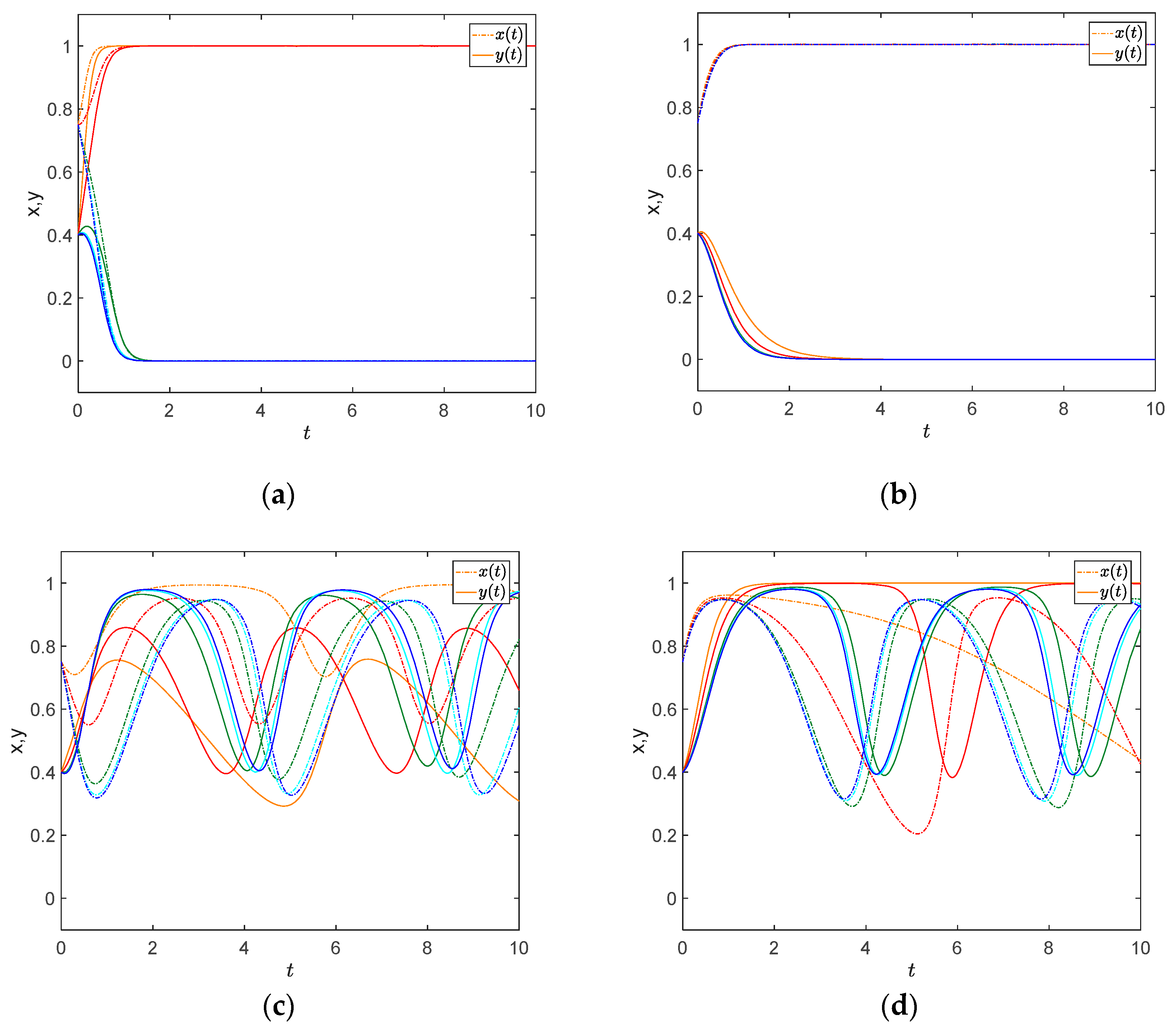
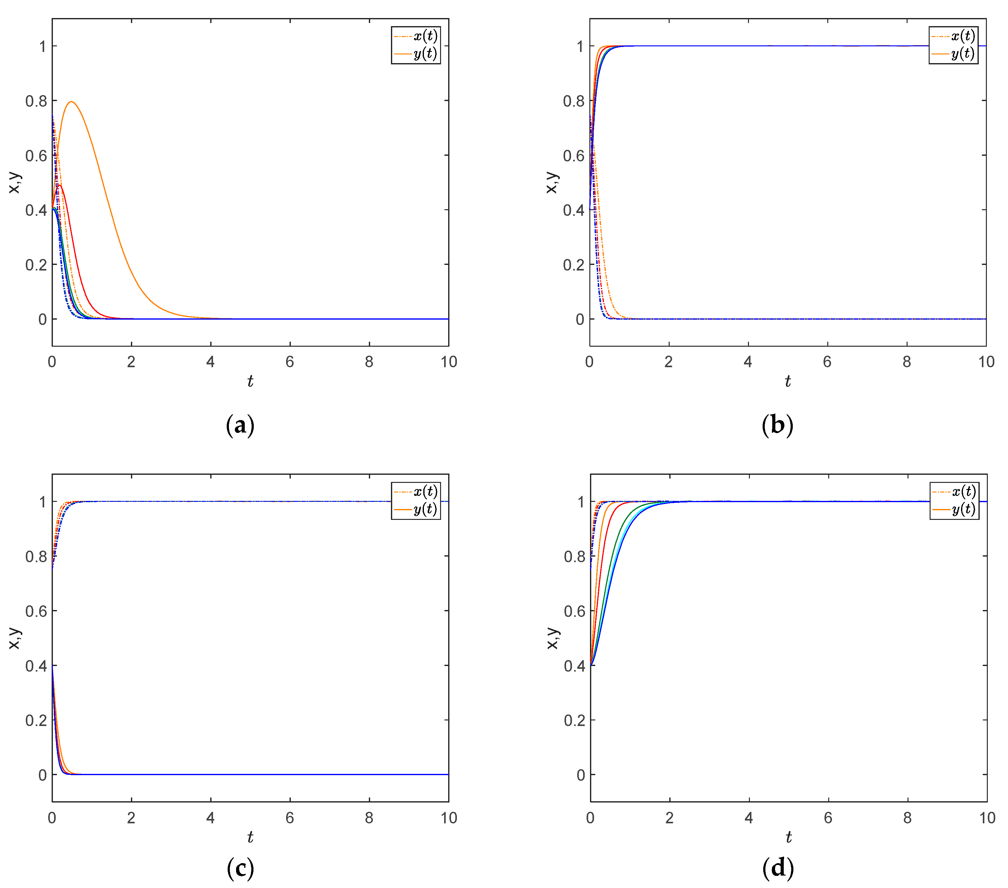
3.2. Impact of the Problem Size

In this section, we will discuss the impact of problem size with respect to the eight scenarios identified by the circled numbers shown in Table 2. To discover how problem size affects the decision making of both players, simulation analysis was carried out for the following five situations: (1) $l=l_0$, where $l_0$ is a very small value allowed by the system (shown in orange curve); (2) $l=2l_0$ (shown in red curve); (3) $l=10l_0$ (shown in green curve); (4) $l=40l_0$ (shown in light blue curve); (5) $l=400l_0$ (shown in blue curve). The dotted line stands for the changing curve of $x$ over time, and the solid line stands for that of $y$. Generally, as the direct beneficiary of the end product, the manufacturer is more willing to deal with the problem in its starting state. However, the supplier is more reluctant to deal with the problem because of fear of sharing cost in its starting state. Hence, we would set the starting point of $x$ to be bigger than 0.5 and that of $y$ to be smaller than 0.5. Moreover, in order to show more clearly in our simulation figures, we set the starting points as $x_0=0.75$ and $y_0=0.4$ in our work.

From Figure 2a, for the scenario where the ESSs of the system are $(0,0)$, $(1,1)$, the following can be observed: (1) Problem size has an effect on the final decisions of both the manufacturer and the supplier. When the size is very small, both players might choose D, but when it is large enough, their final decisions will be N. We think that this can be also easily observed in reality but verified in our simulation. (2) If the size is small enough for both players to choose D, interestingly, hesitation period appears for the supplier as the size increases, but no hesitation period for the manufacturer. We think that, as the direct beneficiary of the end product, the manufacturer would like to deal with the problem when the problem is very small without doubt. However, for the supplier, as the problem size increases, it has to share more and more cost in dealing with the problem. Thus, when the problem size is not enough to influence its payoff, it would rather not to deal with the problem, and the hesitation period arises. Therefore, the cost-sharing ratio may be in some correlation with the hesitation period when the problem size is small and both players would choose D. (3) If the size becomes so large that both players choose N. Interestingly, rather than the supplier, there is a hesitation period for the manufacturer to finally choose N, and when the size increases, the hesitation time becomes shorter. We also think that this phenomenon may have some correlation with the manufacturer as the direct beneficiary of the end product. The manufacturer would not like the problems to cause the loss of its benefit and thus hesitate to solve it. (4) The change rates for both vary only a little, from $l=40l_0$ to $l=400l_0$.

From Figure 2b, for the scenario where the ESSs of the system are $(0,1)$, $(1,0)$, the following can be observed: (1) Changes in problem size have little effect on supplier’s making decisions. (2) The change rate for the manufacturer varies considerably when the problem size changes in the range between $l=l_0$ and $l=10l_0$, but when $l$ is greater than $10l_0$, changes in problem size have little impact on the change rate. This phenomenon is greatly different from what happens in Scenario ①, as shown in Figure 2a. In order to explore the reasons, we make an attempt on the analysis of the following two examples. In the example of Boeing and its angle of attack sensor supplier of 737 project, some potential problems have already been found in the R&D of Boeing aircraft before the two crashes according to CNN. But nothing was taken to solve the problems by either Boeing or the supplier at that time. According to our model and simulation, we may speculate that the problem size was found to be very big then, and this can be seen from the later long-term grounding of the 737 project after the crashes, regardless of the huge loss. In another example of the R&D of C919, COMAC is less experienced than its supplier but show a more active attitude in processing problems than its supplier. In this situation, problem size has nothing to do with the attitudes of the manufacturer and the supplier towards processing the problem. Thus, what happens in Figure 2b is further speculated to happen in the situation of the unbalanced capacity of the manufacturer and the supplier in our work.

From Figure 2c,d we can see that for the scenarios where only the saddle point $(\frac{a_x^{*}}{b_x^{*}},\frac{a_y^{*}}{b_y^{*}})$ exists in the system, changes in problem size affect fluctuation amplitudes and frequencies, but the effect grows smaller as the size becomes larger.

From Figure 3a, for the scenario where the unique ESS $(0,0)$ exists in the system, the following can be observed: (1) The hesitation period for the manufacturer becomes shorter as the problem size increases, and when the size is very large, the manufacturer exhibits almost no hesitation time. As the direct beneficiary of the end product, the manufacturer may have some argument with the supplier about whether to process the problem before finally be persuaded not to deal with the problem. This situation happens frequently in the R&D of C919 in terms of COMAC’s lack of experience. We think that the argument is one reason for the manufacturer’s hesitation, and another reason for the manufacturer’s hesitation is considered to be that the manufacturer may think about a way to deal with the problem on its own first. This kind of situation is more likely to occur with experienced manufacturers, such as Boeing and Airbus. (2) As the problem size becomes large enough, it has little effect on the change rate for either player.

From Figure 3b, for the scenario where the unique ESS $(0,1)$ exists in the system, the following can be observed: (1) When the problem size increases, the change rate for the manufacturer becomes smaller and that for the supplier rises. (2) When the problem size is large enough, changes in its size have little influence on the change rate for either player.

From Figure 3c, for the scenario where the unique ESS $(1,0)$ exists in the system, the following can be observed: (1) When the problem size increases, the change rate for the supplier decreases and that for the manufacturer becomes greater. (2) When the problem size is large enough, changes in its size have little influence on the change rate for either player.

From Figure 3d, for the scenario where the unique ESS $(1,1)$ exists in the system, the following can be observed: (1) When the problem size increases, the change rates for both players become smaller. (2) When the problem size is large enough, changes in its size have little influence on the change rate for either player.

Therefore, what is common in Scenario ① and Scenario ③ to Scenario ⑧, where problem size may affect the final decisions of both the manufacturer and the supplier, is that when the problem size is large enough, changes in the size have little effect on the change rates associated with the decisions. According to the simulation, in the situation of the large size of the problem, the reaction periods for the manufacturer and the supplier have little to do with the change of the problem size. In the example of the 737 project, facing the huge losses caused by two air crashes, both Boeing and its supplier react almost directly on the problem of the 737 project. The problem is so big that it cannot give them enough space to think about it.

The following conclusions can then be drawn based on the above analyses.

Firstly, problem size may have little effect on the final decisions for both players when the experiences or the capacities of the manufacturer and the supplier are unbalanced. This may be due to the inexperienced player’s inability to accurately determine the problem size. Or, two players with different experiences may have disputes about the problem size. Therefore, it is essential for manufacturers and suppliers to accumulate sufficient and effective experience for the R&D of complex products.

Secondly, the existing hesitation periods in our simulation may have some correlation with the following two factors: (1) The cost-sharing ratio between the manufacturer and the supplier, and (2) the role of the manufacturer as the direct beneficiary of the end product. Thus, it is beneficial for the manufacturer to establish a reasonable and effective supplier management system. Besides, a balanced collaborative R&D system is also necessary.

Thirdly, in the situations when the problem size is very small, it is easy for both to choose processing the problem; however, when the problem size increases, both show more reluctance to deal with the problem. We believe that this is why many crashes occurred because the problems had not been effectively processed in the R&D process of the aircraft. Except for the example of what occurred on the 737 project, similar problems happened on Sukhoi Superjet 100 (SSJ100), a regional jet developed by Sukhoi, a Russian aircraft manufacturer, and its suppliers. The crash happened in May 5, 2019 due to a technical problem of SSJ100. To avoid more costs on problem processing and gain much more benefit, the manufacturer and the supplier tend to give up processing the R&D problem and risk to share the benefits, with luck, until bigger problems, like the crash of the aircraft, happen. Thus, to measure how the problem would develop in the R&D of the complex product is also a very important factor when considering the measurement of the problem size.

Fourthly, as the problem size becomes large enough, changes in its size could hardly influence the change rate for either player. The reaction periods for the manufacturer and the supplier becomes so short in this situation that we could hardly observe the change of the reactions. However, as time is so valuable in the R&D of complex products, to establish a good problem reaction system is also considered to be very important, even in the situation of the small problem.

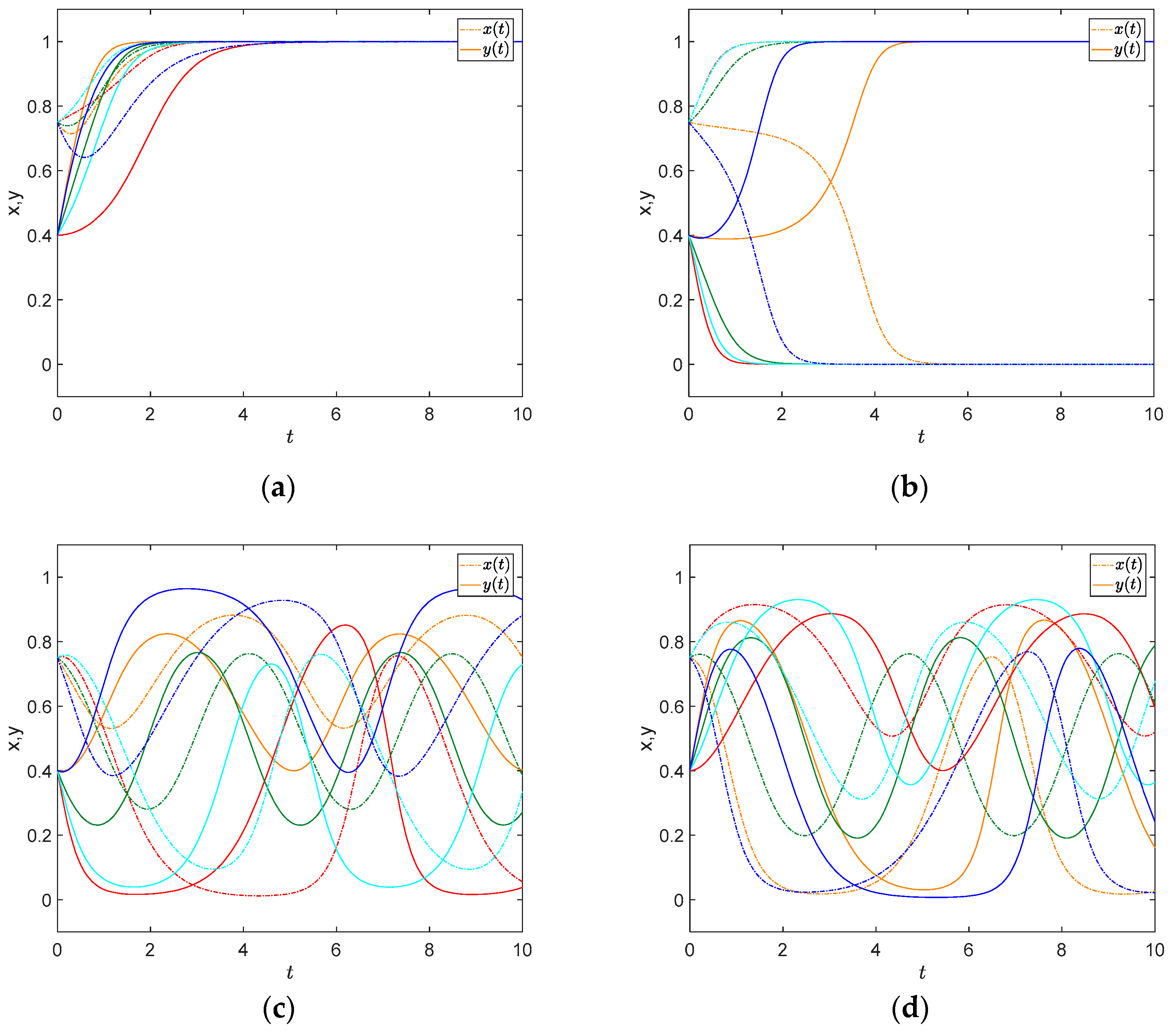
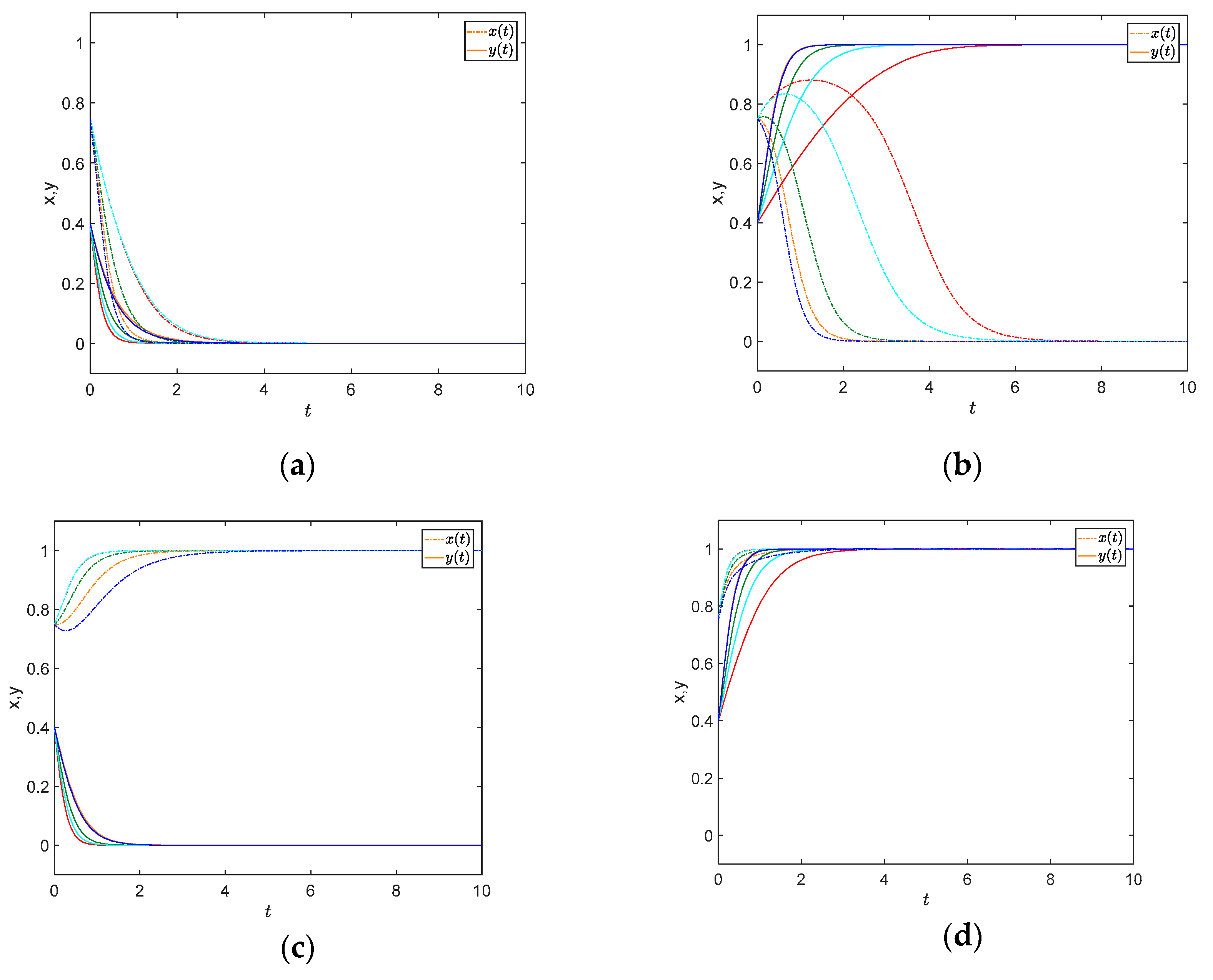
3.3. Impact of The Problem Proposing Mechanism

This section will give a discussion on the impact of the problem proposing mechanism for the eight scenarios that are numbered as shown in Table 2. To detect how the problem proposing mechanism affects the problem processing mechanism, for each scenario, we discuss the following five situations: (1) $p_m=p_s$ (shown in green curve); (2) $p_s$ going up and $p_m$ keeping unchanged on the basis of situation (1) (shown in orange curve); (3) $p_s$ going down and $p_m$ keeping unchanged on the basis of situation (1) (shown in red curve); (4) $p_m$ going up and $p_s$ keeping unchanged on the basis of situation (1) (shown in light blue curve); (5) $p_m$ going down and $p_s$ keeping unchanged on the basis of situation (1) (shown in blue curve). The dotted line stands for the changing curve of $x$ over time, and the solid line stands for that of $y$. In this section we set the starting points of $x$ and $y$ the same as in Section 3.2.

From Figure 4a, for the scenario where the ESSs of the system are $(0,0)$, $(1,1)$, the following can be observed: (1) $p_m$ and $p_s$ have no effect on the final decision of either the manufacturer or the supplier. For Boeing and its supplier, they have almost the same R&D experiences. Thus, their assessments of whether to process a problem are almost the same. Besides, their abilities to identify problems and their evaluations of whether to propose a problem are almost the same. We think that it is this kind of situation when the problem proposing mechanism has little correlation with the problem processing mechanism. (2) The supplier might exhibit a hesitation period, especially when p_s is large enough or $p_m$ is small enough, and when $p_s$ drops or $p_m$ goes up, the probability can go straight to 1 rather than first decreasing. This happens frequently in a relationship with an inexperienced manufacturer like COMAC. The manufacturer is less experienced in dealing with a problem and evaluating the risk of a problem. Two forms of the supplier’s hesitations are considered as below. The supplier may have to think of a way to cooperate with the manufacturer to deal with the problem first until they verify that the problem is invalid. On the other hand, the supplier may argue with the manufacturer as the supplier would be unwilling to share the risk of processing the problem and would rather choose N. (3) For the manufacturer, the increase rate decreases as $p_s$ becomes smaller, and it increases as $p_m$ becomes smaller.

From Figure 4b, for the scenario where the ESSs of the system are $(0,1)$, $(1,0)$, the following can be observed: (1) Changes in $p_m$ or $p_s$ can lead to different final decisions, and when $p_m$ decreases or $p_s$ grows larger, the ESS will transfer from $(1,0)$ to $(0,1)$. In this situation, the probabilities of making decisions for both of them change slowly at first and then directly to the target values. This is completely different from what happens in Scenario ①. In the example of the R&D of C919, the less experienced COMAC would be more likely to propose a problem, and it would also show more willingness to process the problem than its supplier. Thus, we contribute this to the factor of the imbalance of the capacities between the manufacturer and the supplier. We have also noticed that, in this kind of situation, the reaction period is very long. The manufacturer and the supplier may have to spend time examining the existing validity of the proposed problem. (2) If the ESS is $(1,0)$, the change rates for both players increase as $p_m$ increases or $p_s$ decreases.

From Figure 4c,d we can see that for the scenarios where only the saddle point $(\frac{a_x^{*}}{b_x^{*}},\frac{a_y^{*}}{b_y^{*}})$ exists in the system, both $p_m$ and $p_s$ affect fluctuation amplitudes and frequencies.

From Figure 5a, for the scenario where the unique ESS $(0,0)$ exists in the system, when $p_m$ increases or $p_s$ decreases, the change rate for the manufacturer increases while that for the supplier declines.

From Figure 5b, for the scenario where the unique ESS $(0,1)$ exists in the system, the following can be observed: (1) When $p_m$ increases or $p_s$ decreases, a hesitation period appears for the supplier to make a decision. This may happen in the situation when the supplier is primarily responsible for the problem but the manufacturer is experienced in detection of the problem. The supplier would think of a way to avoid D until they have to deal with the problem under some kind of pressure policy, such as the supplier management provisions made by experienced Boeing. (2) When $p_m$ becomes smaller or $p_s$ grows larger, the change rates for both players increase.

From Figure 5c, for the scenario where the unique ESS $(1,0)$ exists in the system, the following can be observed: (1) When $p_m$ declines or $p_s$ grows larger, a hesitation period appears for the supplier to make a decision. This may happen in the situation when the manufacturer is less experienced, like COMAC, but have to try its best to process every problem, even those proposed by the supplier. The supplier may argue with the manufacturer first about the problem processing responsibility after proposing the problem. (2) When $p_m$ increases or $p_s$ decreases, the change rates for both players increase.

From Figure 5d, for the scenario where the unique ESS $(1,1)$ exists in the system, when $p_m$ becomes smaller or $p_s$ becomes larger, the change rate for the manufacturer increases while that for the supplier declines.

Therefore, according to the observations on the decision change rates for the manufacturer and the supplier in Scenario ① to Scenario ⑧, we can get that, to some extent, when the manufacturer demonstrates more willingness to propose the problem and bear the risk, or when the supplier shows greater reluctance to do so, surprisingly, it becomes more difficult for the manufacturer to decide to deal with the problem, but easier for the supplier. With this conclusion, we can give some analysis of the examples of the R&D of the C919 and 737 projects. For the inexperienced COMAC, it may be more likely to propose problems and less experienced in dealing with the problems. But for COMAC’s supplier, it would be more experienced in helping deal with the R&D problems than COMAC as long as the supplier verifies the risk of the proposed problem. Nevertheless, in the R&D of 737, experienced Boeing would rather exert pressure on its supplier about the problems.

Based on all of the above observations, we can then draw the following conclusions.

Firstly, the problem proposing mechanism would hardly influence the final decisions of the manufacturer and the supplier when their capabilities are balanced, which is different from what is explored in the examination of the impact of the problem size. The attempt to establish a balanced collaborative R&D system is effective for the whole supply chain. Thus, as the leader of the R&D process and the direct beneficiary of the end product, the manufacturer should try to make an effective supplier management system.

Secondly, the existing hesitation periods in our simulation about the impact of the problem proposing mechanism may perform in two forms: (1) Argument with the manufacturer, and (2) verification of the reliability of the problem. But both forms are speculated to have correlation with the experience accumulation of the manufacturer in our work. In addition, the accumulation of experience is beneficial for both the manufacturer itself and the supplier, especially in proposing valid problems. This would save time to a large extent, which is extremely important in the R&D of complex products.

Thirdly, the problem proposing mechanism has some correlation with the decision change rates about the problem process mechanism, which is another performing way of the problem reaction periods. We already know that time is precious for the R&D of complex products. Thus, more detailed investigation of the problem processing mechanism is very important for the manufacturer to manage suppliers rationally and organize the R&D process effectively.

4. Discussion

This paper presents an evolutionary game analysis of the impacts of the problem size and the problem proposing mechanism with respect to the processing mechanism of unpredicted problems in a newly-established M-S collaborative system, consisting of one main manufacturer and one supplier. We supposed that, in the problem processing mechanism, both the manufacturer and the supplier could have two strategies, to deal with the problem and not to deal with the problem. They have to make decisions in common without knowing completely about the information of one another in such a newly-established collaboration relationship. Our study contributes to the research literature, with practical implications for the manufacturer and the supplier in the collaboration of R&D of complex products. The main implications of our research conclusions are discussed in the following sections.

4.1. Theoretical Implication

This paper contributes to the collaboration supply chain literature by expanding our understanding of the long-term relationship between the manufacturer and the supplier and the problem processing mechanism under the control of contract. First, this paper sheds light on the importance of the research on the new M-S collaboration system. Prior research have been done on the basis of that the manufacturer and the supplier have been in a long-term relationship between each other [14,24]. However, with the demand of social development, more and more new relationships between the manufacturers and the suppliers are established. In such a newly-established system, we found that both players are not very familiar with each other. They could not know, completely, about each other’s abilities, attitudes, and the environment of their entire supply chain. It will be hard for both of them to make decisions precisely in the R&D process. Thus, evolutionary game theory is applied here, which is reasonable and practical.

Inspired by the issues of air crashes triggered by Boeing 737 MAX 8, and the delayed schedule of C919, we found that in a newly-established M-S collaboration system, unpredicted problems would arise without any advance contract, which is worth focusing on. Prior research focuses on the problem processing mechanism with contracts [15,23]. This paper investigated the problem processing mechanism without consideration of the contracts, and paid more attention to the decision-making behaviors of the manufacturer and the supplier instead. Hu et al. [27] suggested the behaviors that one player deals with the problem solely, both choose to deal with problem, and neither choose to deal with the problem as the research settings. We specified these actions as possible values between 0 and 1, and detected the changing trajectory of these decision probabilities, which is much more figurative in the exploration of the unpredicted problem processing mechanism.

Prior research has shown the influence of the problem size on the profits of the manufacturer and the supplier [36,40]. We assumed the inversely proportional relationship between the problem size and the conversion incomes that are correlated with the problem processing mechanism. We found, in this assumption, that both players are much more willing to deal with the problem according to the observation of simulation. This phenomenon is obvious in practice but has been verified by the model and simulation. Thus, the assumption is reasonable.

Results show that if the problem size changes in an interval with larger values, it may have little effect on the problem processing mechanism, while the problem proposing mechanism always does. Both the problem size and the probability of proposing the problem influence the stability of the decision making when no evolutionary stable strategy exists, because they significantly affect the fluctuation amplitudes and frequencies of the system evolution curves. What is contrary to instinct is the observation that the main manufacturer finds it more difficult than the supplier to make a final decision, when the manufacturer is more likely to propose the problem and bear the risk while the supplier is reluctant to do so. These findings should inspire action with respect to these two factors when the two players find it difficult to make decisions (e.g., control the evaluation of the problem size during attempts to propose the problem).

4.2. Managerial Implication

Our study provides the manufacturer and the supplier in the R&D of complex products with important implications of how to achieve successful collaboration performance in a newly-established M-S system, especially when facing unpredicted problems without contracts beforehand.

Firstly, it is beneficial for the whole supply chain that both sides propose to solve or not to solve the problem together. At the beginning of the collaborative relationship, an equal and transparent negotiation mechanism should be established between the main manufacturer and the supplier. When unpredicted problems arise, they should have a comprehensive evaluation of the problem size through negotiation, and work together to propose solutions.

Secondly, before the manufacturer and the supplier determine the solution to the problem, both the problem size and the problem proposing mechanism have impacts on the decision-making of both sides. In terms of manufacturers hoping to promote the supplier solving the problem, manufacturers should try to communicate to reduce the problem size to some degree, such as changing the product quality goal planning [46]. Additionally, the supplier should cooperate with the manufacturer to put forward problem-solving strategies, collaboratively, as much as possible from the perspective of overall supply-chain revenue and long-term R&D, social benefits, people’s lives, and property security. Besides, according to the conclusion in Section 3.2, we have found that when the problem size is large enough, changes in the size have little effect on the change rates associated with the decisions. However, through what happened in the 737 project, we can get the conclusion that if the problem is big enough to threaten people’s lives, the manufacturer and the supplier should agree on not dealing with the problem but, instead, recalling the end product. Otherwise, the result would not be simply measured by size.

Thirdly, it would be fortunate for the manufacturer to see that, when the manufacturer discovers and proposes the problem, the supplier will be very willing to solve the problem even if the manufacturer is not able to do so. Thus, from the perspective of management, the manufacturer should try to play a role as a leader and persuade the supplier to be its follower in the R&D process, like Boeing and its supplier.

Last but not least, the hesitation period found in Section 3.2 and in Section 3.3 is worth paying attention to here. Combined with the simulation conclusions and the analysis of the examples of the C919 and 737 projects, we find that the accumulation of experience and a pressure policy is very important for the manufacturer in managing its suppler.

4.3. Limitations and Future Research Directions

As we have found, the experience of the manufacturer is an important effect on the attitudes of both the manufacturer and the supplier toward processing the problem. But the hesitation period exists actually as a form of contradiction between the manufacturer and the supplier. Thus, the balance between the experience and the attitude should be taken into extended research that is practical and reasonable. Additionally, we derived the conclusion of Section 3.3 that if one player propose the problem, it would share much more risk in proposing the problem as well as processing the problem. Therefore, another extended consideration of our work should also focus on the suitable cost-sharing ratio to make both players willing to solve the problem at the same time, which is also an important factor when considering the hesitation period during exploration of the impact of the problem size in Section 3.2.

Future study of the problem processing mechanism should be conducted with the goal of explaining the reasons for this result of the comparison analysis, between the probabilities of proposing a problem and processing the problem. It will be very interesting to consider what will happen if the consumer is added as a third player in the model. Here, some new problems may arise, for example, consumer demand will play as a factor in affecting the attitudes of the manufacturer and the supplier towards processing the problem. In addition, while we consider the strategies the manufacturer and the supplier choose, the factor of the consumer assessment of the product quality could lead to additional insights.

Moreover, as the idea of M-S mode has also achieved some considerable success in other fields besides the complex product R&D in recent years, such as waste proposal [47], medicine [48], internet retailing [49], and so on, we can also get some implications on the unpredicted problem processing mechanism in a new M-S collaborative system when considering the management of these fields.

References

1. Lambert, A.J.D. Optimal disassembly of complex products. Int. J. Prod. Res. 1997, 35, 2509–2524. [Google Scholar] [CrossRef] [Green Version]
2. Lewis, C. A Case Study in the Use of Computer-Based Training in Statistical Process Control. J. Oper. Res. Soc. 1986, 37, 669–675. [Google Scholar] [CrossRef]
3. Delbridge, R.; Oliver, N. Narrowing the gap? Stock turns in the Japanese and Western car industries. Int. J. Prod. Res. 1991, 29, 2083–2095. [Google Scholar] [CrossRef]
4. Paknejad, M.J.; Nasri, F.; Affisco, J.F. Lead-time variability reduction in stochastic inventory models. Eur. J. Oper. Res. 1992, 62, 311–322. [Google Scholar] [CrossRef]
5. Akai, K.; Sakamoto, K.; Nishino, N.; Kageyama, K. Game Theoretic Analysis of Exclusive Contract for Carbon Fiber Reinforced Plastic in the Aviation Industry. Procedia CIRP 2016, 41, 1043–1048. [Google Scholar] [CrossRef] [Green Version]
6. Golmohammadi, A.; Taghavi, M.; Farivar, S.; Azad, N. Three strategies for engaging a buyer in supplier development efforts. Int. J. Prod. Econ. 2018, 206, 1–14. [Google Scholar] [CrossRef]
7. Baptista, S.; Barbosa-Póvoa, A.P.; Escudero, L.F.; Gomes, M.I.; Pizarro, C. On risk management of a two-stage stochastic mixed 0–1 model for the closed-loop supply chain design problem. Eur. J. Oper. Res. 2019, 274, 91–107. [Google Scholar] [CrossRef]
8. Chan, C.K.; Fang, F.; Langevin, A. Single-vendor multi-buyer supply chain coordination with stochastic demand. Int. J. Prod. Econ. 2018, 206, 110–133. [Google Scholar] [CrossRef]
9. Chintapalli, P.; Disney, S.M.; Tang, C.S. Coordinating Supply Chains via Advance-Order Discounts, Minimum Order Quantities, and Delegations. Prod. Oper. Manag. 2017, 26, 2175–2186. [Google Scholar] [CrossRef] [Green Version]
10. Wlazlak, P.; Säfsten, K.; Hilletofth, P. Original equipment manufacturer (OEM)-supplier integration to prepare for production ramp-up. J. Manuf. Technol. Manag. 2019, 30, 506–530. [Google Scholar] [CrossRef]
11. Erfurth, T.; Bendul, J. Integration of global manufacturing networks and supply chains: A cross case comparison of six global automotive manufacturers. Int. J. Prod. Res. 2018, 56, 7008–7030. [Google Scholar] [CrossRef]
12. Nosoohi, I.; Nookabadi, A.S. Outsource planning with asymmetric supply cost information through a menu of option contracts. Int. Trans. Oper. Res. 2019, 26, 1422–1450. [Google Scholar] [CrossRef]
13. Dwaikat, N.Y.; Money, A.H.; Behashti, H.M.; Salehi-Sangari, E. How does information sharing affect first-tier suppliers’ flexibility? Evidence from the automotive industry in Sweden. Prod. Plan. Control 2018, 29, 289–300. [Google Scholar] [CrossRef]
14. Zhang, M.; Guo, H.; Huo, B.; Zhao, X.; Huang, J. Linking supply chain quality integration with mass customization and product modularity. Int. J. Prod. Res. 2019, 207, 227–235. [Google Scholar] [CrossRef]
15. Patra, P.; Kumar, U.D.; Nowicki, D.R.; Randall, W.S. Effective management of performance-based contracts for sustainment dominant systems. Int. J. Prod. Res. 2019, 208, 369–382. [Google Scholar] [CrossRef]
16. Tang, O.; Musa, S.N. Identifying risk issues and research advancements in supply chain risk management. Int. J. Prod. Res. 2011, 133, 25–34. [Google Scholar] [CrossRef] [Green Version]
17. Gintis, H. Game Theory Evolving: A Problem-Centered Introduction to Modeling Strategic Behavior; Princeton University Press: Princeton, NJ, USA, 2000. [Google Scholar]
18. Strull, G. The coming challenge of lsi. In Proceedings of the Aerospace & Electronic Systems and Communications Technology Groups National Telemetering Conference, Amsterdam, The Nederland, 28–29 April 1969; p. 327. [Google Scholar]
19. Tang, C.S.; Yang, S.A.; Wu, J. Sourcing from suppliers with financial constraints and performance risk. Manuf. Serv. Oper. Manag. 2017, 20, 70–84. [Google Scholar] [CrossRef]
20. Li, S.; Zhao, X.; Huo, B. Supply chain coordination and innovativeness: A social contagion and learning perspective. Int. J. Prod. Res. 2018, 205, 47–61. [Google Scholar] [CrossRef]
21. Liu, Z.; Wang, J. Supply chain network equilibrium with strategic supplier investment: A real options perspective. Int. J. Prod. Res. 2019, 208, 184–198. [Google Scholar] [CrossRef]
22. Zhang, C.; Fang, D.; Yang, X.; Zhang, X. Push and pull strategies by component suppliers when OEMs can produce the component in-house: The roles of branding in a supply chain. Ind. Market. Manag. 2018, 72, 99–111. [Google Scholar] [CrossRef]
23. Hu, B.; Qi, A. Optimal procurement mechanisms for assembly. Manuf. Serv. Oper. Manag. 2018, 20, 655–666. [Google Scholar] [CrossRef]
24. Wu, X.; Zhou, Y. Buyer-specific versus uniform pricing in a closed-loop supply chain with third-party remanufacturing. Eur. J. Oper. Res. 2019, 273, 548–560. [Google Scholar] [CrossRef]
25. He, J.; Ma, C.; Pan, K. Capacity investment in supply chain with risk averse supplier under risk diversification contract. Transp. Res. Part E Logist. Transp. Rev. 2017, 106, 255–275. [Google Scholar] [CrossRef]
26. Nikoofal, M.E.; Gümüş, M. Quality at the source or at the end? Managing supplier quality under information asymmetry. Manuf. Serv. Oper. Manag. 2018, 20, 498–516. [Google Scholar] [CrossRef]
27. Hu, J.; Hu, Q.; Xia, Y. Who should invest in cost reduction in supply chains? Int. J. Prod. Res. 2019, 207, 1–18. [Google Scholar] [CrossRef]
28. Nakkas, A.; Xu, Y. The Impact of Valuation Heterogeneity on Equilibrium Prices in Supply Chain Networks. Prod. Oper. Manag. 2019, 28, 241–257. [Google Scholar] [CrossRef]
29. Braziotis, C.; Tannock, J.D.; Bourlakis, M. Strategic and operational considerations for the Extended Enterprise: Insights from the aerospace industry. Prod. Plan. Control 2017, 28, 267–280. [Google Scholar] [CrossRef]
30. Tong, X.; Chen, J.; Zhu, Q.; Cheng, T.C.E. Technical assistance, inspection regime, and corporate social responsibility performance: A behavioural perspective. Int. J. Prod. Res. 2018, 206, 59–69. [Google Scholar] [CrossRef]
31. Bai, C.; Sarkis, J. Honoring complexity in sustainable supply chain research: A rough set theoretic approach (SI: ResMeth). Prod. Plan. Control 2018, 29, 1367–1384. [Google Scholar] [CrossRef]
32. Li, X.; Chen, J.; Ai, X. Contract design in a cross-sales supply chain with demand information asymmetry. Eur. J. Oper. Res. 2019, 275, 939–956. [Google Scholar] [CrossRef]
33. Zhuo, W.; Shao, L.; Yang, H. Mean-variance analysis of option contracts in a two-echelon supply chain. Eur. J. Oper. Res. 2018, 271, 535–547. [Google Scholar] [CrossRef]
34. Huang, Q.; Yang, S.; Shi, V.; Zhang, Y. Strategic decentralization under sequential channel structure and quality choices. Int. J. Prod. Res. 2018, 206, 70–78. [Google Scholar] [CrossRef]
35. He, Q.; Wang, N.; Yang, Z.; He, Z.; Jiang, B. Competitive collection under channel inconvenience in closed-loop supply chain. Eur. J. Oper. Res. 2019, 275, 155–166. [Google Scholar] [CrossRef]
36. Levner, E.; Ptuskin, A. Entropy-based model for the ripple effect: Managing environmental risks in supply chains. Int. J. Prod. Res. 2018, 56, 2539–2551. [Google Scholar] [CrossRef]
37. Awasthi, A.; Chauhan, S.S.; Goyal, S.K.; Proth, J.M. Supplier selection problem for a single manufacturing unit under stochastic demand. Int. J. Prod. Res. 2009, 117, 229–233. [Google Scholar] [CrossRef]
38. Giri, B.C.; Bardhan, S. Sub-supply chain coordination in a three-layer chain under demand uncertainty and random yield in production. Int. J. Prod. Res. 2017, 191, 66–73. [Google Scholar] [CrossRef]
39. Yeung, W.K.; Choi, T.M.; Cheng, T.C.E. Supply chain scheduling and coordination with dual delivery modes and inventory storage cost. Int. J. Prod. Res. 2011, 132, 223–229. [Google Scholar] [CrossRef]
40. Aljazzar, S.M.; Jaber, M.Y.; Moussawi-Haidar, L. Coordination of a three-level supply chain (supplier–manufacturer–retailer) with permissible delay in payments. Appl. Math. Model. 2016, 40, 9594–9614. [Google Scholar] [CrossRef]
41. Xiao, T.; Chen, G. Wholesale pricing and evolutionarily stable strategies of retailers with imperfectly observable objective. Eur. J. Oper. Res. 2009, 196, 1190–1201. [Google Scholar] [CrossRef]
42. Yi, Y.; Yang, H. Wholesale pricing and evolutionary stable strategies of retailers under network externality. Eur. J. Oper. Res. 2017, 259, 37–47. [Google Scholar] [CrossRef]
43. Wang, L.; Zheng, J. Research on low-carbon diffusion considering the game among enterprises in the complex network context. J. Clean. Prod. 2019, 210, 1–11. [Google Scholar] [CrossRef]
44. Weibull, J.W. Evolutionary Game Theory; The MIT Press: Cambridge, MA, USA, 1995. [Google Scholar]
45. Friedman, D. Evolutionary games in economics. Econometrica 1991, 59, 637–666. [Google Scholar] [CrossRef]
46. Trautrims, A.; MacCarthy, B.L.; Okade, C. Building an innovation-based supplier portfolio: The use of patent analysis in strategic supplier selection in the automotive sector. Int. J. Prod. Res. 2017, 194, 228–236. [Google Scholar] [CrossRef] [Green Version]
47. Dinis-Carvalho, J.; Moreira, F.; Bragança, S.; Costa, E.; Alves, A.; Sousa, R. Waste identification diagrams. Prod. Plan. Control 2015, 26, 235–247. [Google Scholar]
48. Chick, S.E.; Hasija, S.; Nasiry, J. Information elicitation and influenza vaccine production. Oper. Res. 2016, 65, 75–96. [Google Scholar] [CrossRef]
49. Ibrahim, M.F. Integration of three echelon supply chain (supplier-manufacturer-distributor-drop shipper) with permissible delay in payment and penalty contract. In IOP Conference Series: Materials Science and Engineering; IOP Publishing: Bristol, UK, 2018; Volume 337, p. 012027. [Google Scholar]
Figure 1. Conceptual research model.
Mathematics 07 00588 g001
Figure 2. Evolution curves of the system (I) with different problem sizes in the scenarios in which the saddle point s p (We abbreviate the saddle point ( a x * b x * , a y * b y * ) as s p for format convenience.) exists. (a) Scenario ①; (b) Scenario ②; (c) Scenario ③ and (d) Scenario ④.
Mathematics 07 00588 g002
Figure 3. Evolution curves of the system (I) with different problem sizes in the scenarios in which the saddle point s p does not exist. (a) Scenario ⑤; (b) Scenario ⑥; (c) Scenario ⑦ and (d) Scenario ⑧.
Mathematics 07 00588 g003
Figure 4. Evolution curves of the system (I) with different proposing probabilities in the scenarios in which the saddle point s p exists. (a) Scenario ①; (b) Scenario ②; (c) Scenario ③ and (d) Scenario ④.
Mathematics 07 00588 g004
Figure 5. Evolution curves of the system (I) with different proposing probabilities in the scenarios in which the saddle point s p does not exist. (a) Scenario ⑤; (b) Scenario ⑥; (c) Scenario ⑦ and (d) Scenario ⑧.
Mathematics 07 00588 g005