Solutions of Direct and Inverse Even-Order Sturm-Liouville Problems Using Magnus Expansion

Abstract

In this paper Lie group method in combination with Magnus expansion is utilized to develop a universal method applicable to solving a Sturm–Liouville problem (SLP) of any order with arbitrary boundary conditions. It is shown that the method has ability to solve direct regular (and some singular) SLPs of even orders (tested for up to eight), with a mix of (including non-separable and finite singular endpoints) boundary conditions, accurately and efficiently. The present technique is successfully applied to overcome the difficulties in finding suitable sets of eigenvalues so that the inverse SLP problem can be effectively solved. The inverse SLP algorithm proposed by Barcilon (1974) is utilized in combination with the Magnus method so that a direct SLP of any (even) order and an inverse SLP of order two can be solved effectively.

1. Introduction

Direct and inverse eigenvalue problems (EVP) of linear differential operators play an important role in all vibration problems in engineering and physics [1]. The theory of direct Sturm–Liouville problems (SLP) started around the 1830s in the independent works of Sturm and Liouville.The inverse Sturm–Liouville theory originated in 1929 [2].

In this paper, we consider the $2m$th order, nonsingular, self-adjoint eigenvalue problem:

$$\begin{array}{c}{(-1)}^m{(p_m(x)y^{(m)})}^{(m)}+{(-1)}^{m-1}{(p_{m-1}(x)y^{(m-1)})}^{(m-1)}\\ +\dots +{(p_2(x)y^{″})}^{″}-{(p_1(x)y^{\prime })}^{\prime }+p_0(x)y=\lambda w(x)y,a<x<b\end{array}$$

(1)

along with y satisfying some general, separated boundary conditions at a and b (see Equation (2)). Usually, the functions $p_k,(0\le k\le m)$, and $w(x)$ are continuous on the finite closed interval $[a,b]$, and $p_m$ has continuous derivative. Further assumptions A1–A4 are placed on the coefficient functions in Section 2.1. For Equation (1), the direct eigenvalue problems is concerned with determining the $\lambda$ given the coefficient information $p_k$, $(0\le k\le m)$, and the inverse eigenvalue problem is concerned with reconstructing the unknown coefficient functions $p_k$, $(0\le k\le m)$ from the knowledge of suitable spectral data satisfying the equation.

There is a variety of numerical solutions for the simplest case of Equation (1) known as the direct Sturm–Liouville problem with $m=1$, the most notable ones being Finite difference method (FDM) [3], Numerov’s method (NM) [4], Finite element method (FEM) [5], Modified Numerov’s method (MNM) [6], FEM with trigonometric hat functions using Simpson’s rule (FEMS) and using trapezoidal rule (FEMT) [7], Lie-Group methods (LGM) [8], MATSLISE [9], Magnus integrators (MI) [10], and Homotopy Perturbation Method (HPM)  [11].

For a discussion on numerical methods for inverse SLP, refer to Freiling and Yurko [12]. McLaughlin [13] provided an overview of analytical methods for second- and fourth-order inverse problems. For the inverse SLP, some available methods are iterative solution (IS) [14] and Numerov’s method (NM) [15].

Slightly fewer techniques are available for the direct eigenvalue problem of case $m=2$ known as fourth-order Sturm–Liouville problem (FSLP). For example, Adomian decomposition method (ADM) [16], Chebyshev spectral collocation method (CSCM) [17], Homotopy Perturbation Method (HPM) [11], homotopy analysis method (HAM) [18], Differential quadrature method (DQM) and Boubaker polynomials expansion scheme (BPES) [19], Chebychev method (CM)  [20], Spectral parameter power series (SPPS) [21], Chebyshev differentiation matrices (CDM) [22], variational iteration method (VIM) [23], Matrix methods (MM) [24], and Lie Group method [25] are the prominent techniques available.

Among others Barcilon [26], and McLaughlin [27,28] proposed numerical algorithms for solving the inverse FSLP.

Several methods are available for $m=3$, or Sixth-order SLP (SSLP). They are shooting method [29], Chebyshev spectral collocation method (CSCM) [17], Adomian decomposition method (ADM) [30], and Chebyshev polynomials (CP) [31].

However, as the order of the direct problem increases, it becomes much harder to solve and also the accuracy of the eigenvalues decreases with the index since only a small portion of numerical eigenvalues are reliable [32].

All of the above-mentioned methods are applicable only to a particular order of the SLP and specific set(s) of boundary conditions. In contrast, in this paper, the Lie group method in combination with the Magnus expansion is utilized to construct a method applicable to solving any order of SLP with arbitrary boundary conditions, which was initially applied for solving SLP by Moan [8] and Ledoux et al. [10] and FSLP by Mirzaei [25]. The proposed method is universal in the sense that it can be applied to solve a SLP of any (even) order with different types of boundary conditions (including some singular) subject to computational feasibility inherent to large matrix computations.

The inverse problem is much harder as restrictions on the spectral data should be placed to ensure the uniqueness. Barcilon [33] proved that, in general, $m+1$ spectra associated with $m+1$ distinct “admissible” boundary conditions are required to determine $p_m$’s uniquely (with $p_m=w=1$). Later, McLaughlin and Rundell [34] proved that the measurement of a particular eigenvalue for an infinite set of different boundary conditions is sufficient to determine the unknown potential. Both these theorems an infinite number of accurate eigenvalue measurements, which are hard to obtain in practice as the higher eigenvalues are usually more expensive to compute than lower ones [35]. However, the present technique can be applied to address some of the above difficulties in finding suitable set(s) of eigenvalues so that the inverse problem can be effectively solved.

Section 2 describes the method constructed using the Lie group method in combination with the Magnus expansion and Section 3 provides some numerical examples of direct Sturm–Liouville problems of different orders $m=1,2,3,4$ with a variety of (including one singular) boundary conditions. Furthermore, the efficiency and accuracy of the proposed technique is illustrated, using Example 1. Section 4 presents two examples of Inverse SLP of order two with a symmetric and a non-symmetric potential. Finally, Section 5 concludes with discussion and a summary.

2. Materials and Methods

2.1. Notations

In this paper, Equation (1) is considered under the assumptions:

A1: 

All coefficient functions are real valued.

A2: 

Interval $(a,b)$ is finite.

A3: 

The coefficient functions $p_k$, $(0\le k\le m-1)$, w and $1/p_m$ are in $L^1(a,b)$.

A4: 

Infima of $p_m$ and w are both positive.

(The last two assumptions, A3 and A4, are relaxed in Example 3.) By Greenberg and Marletta [29], provided the above assumptions are true, one gets:

R1: 

The eigenvalues are bounded below.

R2: 

The eigenvalues can be ordered: ${\lambda }_0\le {\lambda }_1\le {\lambda }_2\le \dots$.

R3: 

${lim}_{k\to \infty }{\lambda }_k=+\infty$.

Defining quasi-derivatives:

$$\begin{array}{cc}\hfill u_k& =y^{(k-1)},1\le k\le m,\hfill \\ \hfill v_1& ={(-1)}^m{p}_m{y}^{(m)},\hfill \\ \hfill v_2& ={(-1)}^m{(p_m{y}^{(m)})}^{\prime }+{(-1)}^{m-1}(p_{m-1}{y}^{(m-1)}),\hfill \\ & ⋮\hfill \\ \hfill v_k& ={(-1)}^m{(p_m{y}^{(m)})}^{(k-1)}+{(-1)}^{m-1}{(p_{m-1}{y}^{(m-1)})}^{(k-2)}+\dots +{(-1)}^{m-k+1}(p_{m-1}{y}^{(m-k+1)}),\hfill \\ & ⋮\hfill \\ \hfill v_2& =p_2{y}^{″}-{(p_3{y}^{\prime \prime \prime })}^{\prime }+{(p_4{y}^{(4)})}^{″}+\dots +{(-1)}^{m-2}{(p_m{y}^{(m)})}^{(m-2)},\hfill \\ & ⋮\hfill \\ \hfill v_m& ={(-1)}^{m-1}{(p_m{y}^{(m)})}^{(m-1)}+\dots -{(p_3{y}^{\prime \prime \prime })}^{″}+{(p_2{y}^{″})}^{\prime }-p_1{y}^{\prime },\hfill \end{array}$$

the general, separated, self-adjoint boundary conditions can be written in the form [29]:

$$\begin{array}{cc}\hfill A_{1}u(a)+A_{2}v(a)=0,& B_{1}u(b)+B_{2}v(b)=0,\hfill \end{array}$$

(2)

where

• $A_1,A_2,B_1,B_2$ are $m\times m$ real matrices;
• $A_1{A}_2^T=A_2{A}_1^T$ and $B_1{B}_2^T=B_2{B}_1^T$; and
• $m\times 2m$ matrices $(A_1:A_2)$ and $(B_1:B_2)$ have rank m.

Equation (1) in the matrix form is:

$$\begin{array}{cc}\hfill U^{\prime }=G(x)U& \hfill \end{array}$$

(3)

$$\begin{array}{cc}\hfill AU(a)+BU(b)& =0\hfill \end{array}$$

(4)

with

$$\begin{array}{cc}\hfill G(x)& ={\left(\begin{array}{cccccccccc}0& 1& 0& 0& 0& 0& 0& 0& 0& 0\\ 0& 0& 1& 0& 0& 0& 0& 0& 0& 0\\ 0& 0& 0& \ddots & 0& 0& 0& 0& 0& 0\\ 0& 0& 0& 0& 1& 0& 0& 0& 0& 0\\ 0& 0& 0& 0& 0& 1/p_m(x)& 0& 0& 0& 0\\ 0& 0& 0& 0& p_{m-1}(x)& 0& 1& 0& 0& 0\\ 0& 0& 0& 0& 0& 0& 1& 0& 0\\ 0& 0& p_2(x)& 0& 0& 0& 0& 0& \ddots & 0\\ 0& p_1(x)& 0& 0& 0& 0& 0& 0& 0& 1\\ \lambda w(x)-p_0(x)& 0& 0& 0& 0& 0& 0& 0& 0& 0\end{array}\right)}_{2m\times 2m}\hfill \end{array}$$

(5)

$$\begin{array}{cc}\hfill U& =[u_1,u_2,\dots ,u_m,v_1,v_2,\dots ,v_m],\hfill \\ \hfill A& =\left(\begin{array}{cc}{A}_1& A_2\\ 0_m& 0_m\end{array}\right),B=\left(\begin{array}{cc}{0}_m& 0_m\\ B_1& B_2\end{array}\right).\hfill \end{array}$$

2.2. Lie Algebra

The Lie group $(G,·)$ was introduced by Lie [36] as a differentiable manifold with the algebraic structure of a group. The tangent space at identity is called the Lie algebra of G and denoted by $\mathbf{g}$. A binary operation $[·,·]:\mathbf{g}\times \mathbf{g}\to \mathbf{g}$ is called a Lie bracket. Let $x,y\in \mathbf{g}$, then the Lie bracket $[x,y]$ is defined as:

$$\begin{array}{cc}\hfill [x,y]& =xy-yx.\hfill \end{array}$$

(6)

Special Lie group is defined as

$$\begin{array}{c}\hfill SL(F,n)=\{y\in F^{n\times n},det(y)=1\}.\end{array}$$

(7)

A system of linear ordinary differential equations on $SL(F,n)$ has the form [37]:

$$\begin{array}{cc}\hfill y^{\prime }=G(x)y,& tr(G(x))=0\iff det(y)=1.\hfill \end{array}$$

(8)

Letting $U(x)=Y(x)U(a)$, where $U(a)$ represents the initial data, $Y(x)$ satisfies the differential equation

$$\begin{array}{cc}\hfill Y^{\prime }(x)& =G(x)Y(x),Y(a)=I\hfill \end{array}$$

(9)

where I stands for the $n-$dimensional identity matrix [38]. Since $tr(G(x))=0$, we have $detY(x)=1$, so that Equation (8) is on the Lie Group $SL({\mathbb{R}}^4,4)$, hence can be solved by the Magnus expansion. Let $Y(x)$ be a solution of Equation (9) for $x\ge a$; the solution of the system in Equation (3) with initial condition $U(a)$ is

$$\begin{array}{cc}\hfill U(x)& =Y(x)U(a).\hfill \end{array}$$

Thus, $U(b)=Y(b)U(a)$ and using boundary conditions in Equation (4):

$$\begin{array}{cc}\hfill AU(a)+BY(b)U(a)=0& \Rightarrow [A+BY(b)]U(a)=0.\hfill \end{array}$$

Here, $U(a)\ne 0$. Hence, the eigenvalues $\lambda$ of the SLP in Equation (1) are the roots of the characteristic equation:

$$\begin{array}{cc}\hfill F(\lambda )& =det(A+BY(b))=0.\hfill \end{array}$$

(10)

As the problem in Equation (1) is self-adjoint, the roots of Equation (10) are simple [14], hence can be calculated using the bisection method or any other root finding method. Although an explicit expression for $F(\lambda )$ cannot be found, we can find the roots by computing $F(\lambda )$ for a real number $\lambda$. Besides, one can plot the function $F(\lambda )$ to get an idea of the locations of the roots, and to specify a smaller bracket for the bisection method, thus increasing the efficiency of the method. However, the slow convergence and high computational time requirements make it impossible to use the bisection method, especially when it comes to higher-order SLPs. As the explicit form of F (and its derivatives) is unknown, a Newton-like method cannot apply. To overcome these difficulties, we propose an alternative root finding method in the following paragraph.

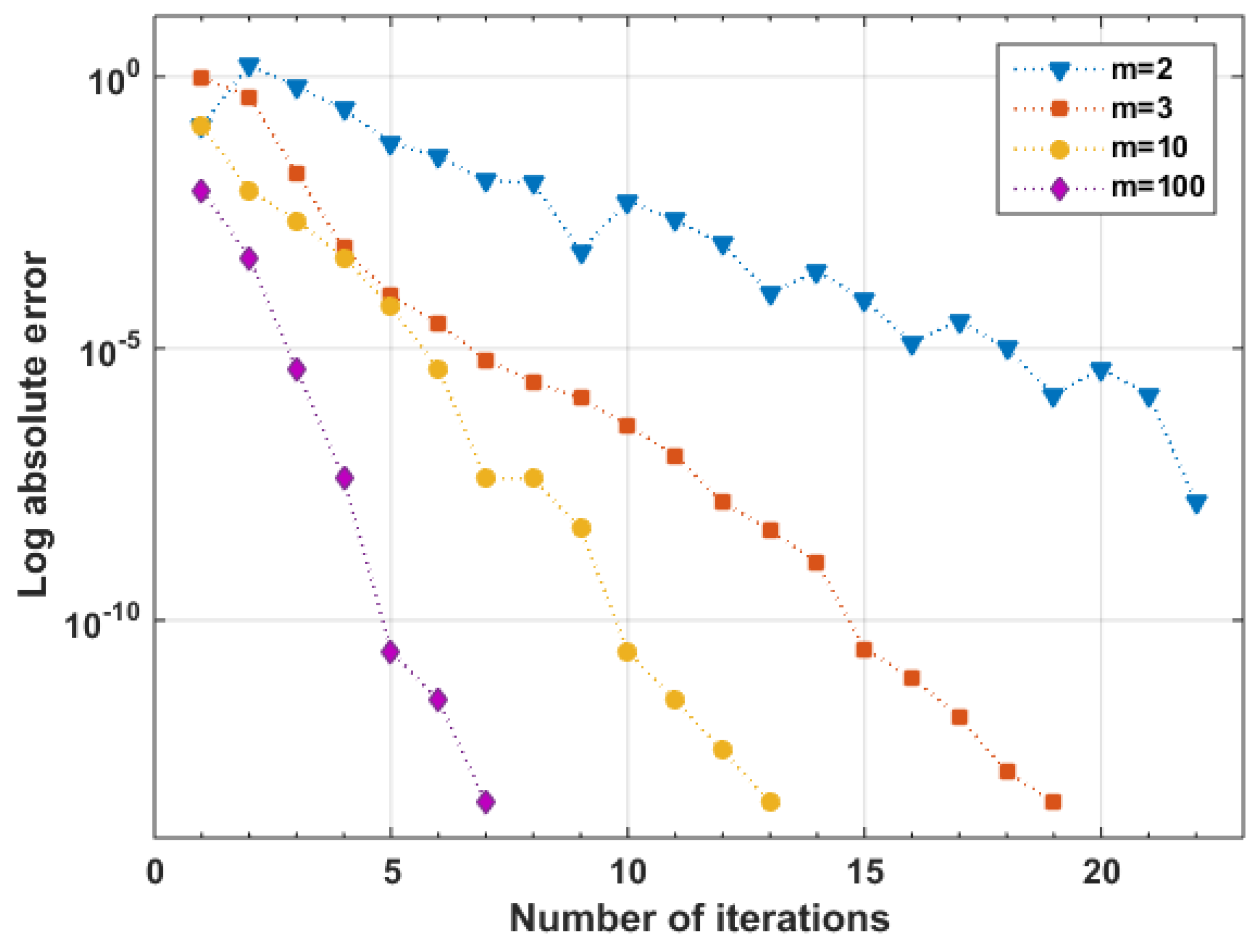
2.3. Multisection Method

A new root finding method, named “Multisection method”—a variant of the bisection method—is proposed, which can converge to the desired root faster. The idea is to divide the root interval into m subsections ($m=2$ being the bisection method) and locate the sign changing interval. Then, this interval is again refined into m subsections and the sign changing interval is located. This continues until the desired accuracy or the maximum number of iterations is reached (See Example A1 in Appendix A, which illustrates the usage and the performance of multisection method.)

This method overcomes drawbacks in the bisection method, yet provides a simple and faster, derivative-free solution to the root-finding problem. This method is able to find even multiple roots in an interval, and, given a sufficiently small subsection length, it is able to find roots that are cluster closer to each other (see Example 4). Unlike the bisection method, this method does not require the bracketing interval to have different signs at the endpoints. In the present paper, the input to this method is a set of function values, as it does not require specifying the explicit functional form of F, which is another advantage of this method. Due to the faster convergence of the multisection method (even at the risk of more computational cost), it can be used to find the eigenvalues (or roots) of the characteristic function.

2.4. Magnus Expansion

Magnus [39] proposed a solution to Equation (8) as

$$\begin{array}{cc}\hfill y(x)& =exp\mathsf{\Omega }(x)y(a),\hfill \end{array}$$

(11)

and a series expansion for the exponent

$$\begin{array}{cc}\hfill \mathsf{\Omega }(x)& =\sum _{k=1}^{\infty }{\mathsf{\Omega }}_k(x),\hfill \end{array}$$

(12)

which is called the Magnus expansion. Its first term can be written as

$$\begin{array}{cc}\hfill {\mathsf{\Omega }}_1(x)& ={\int }_0^{x}G(t_1)d{t}_1\hfill \\ \hfill {\mathsf{\Omega }}_2(x)& =\frac{1}{2}{\int }_0^{x}d{t}_1{\int }_0^{t_2}d{t}_2[G(t_1),G(t_2)]\hfill \\ \hfill {\mathsf{\Omega }}_3(x)& =\frac{1}{6}{\int }_0^{x}d{t}_1{\int }_0^{t_1}d{t}_2{\int }_0^{t_2}d{t}_3[G(t_1),[G(t_2),G(t_3)]]+[G(t_3),[G(t_2),G(t_1)]]\hfill \\ \hfill ⋮& =⋮\hfill \end{array}$$

where $[A,B]\equiv AB-BA$ is the matrix commutator of A and B.

2.5. Numerical Procedure

The Magnus series only converges locally, hence, to calculate $\mathsf{\Omega }$, the interval $[a,b]$ should be divided into N steps such that the Magnus series converges in each subinterval $[x_{n-1},x_n]$, $n=1,\dots ,N$, with $x_N=b$.

Then, the solution at $x_N$ is represented by

$$\begin{array}{cc}\hfill Y(x_N)& =\prod _{n=1}^{N}exp(\mathsf{\Omega }(x_{n-1},x_n))Y_0,\hfill \end{array}$$

(13)

and the series $\mathsf{\Omega }(x_{n-1},x_n)$ has to be appropriately truncated.

The three steps in the procedure are:

E1: 

$\mathsf{\Omega }$ series is truncated at an appropriate order: For achieving an integration method of order $2s(s>1)$ only terms up to ${\mathsf{\Omega }}_{2s-2}$ in the $\mathsf{\Omega }$ series are required [38].

E2: 

The multivariate integrals in the truncated series ${\mathsf{\Omega }}^{\left[p\right]}={\sum }_{i=1}^p{\mathsf{\Omega }}_p$ are replaced by conveniently chosen approximations: if their exact evaluation is not possible or is computationally expensive, a numerical quadrature may be used instead. Suppose that $b_i,c_i,(i=1,\dots ,k)$ are the weights and nodes of a particular quadrature rule, say X of order p, respectively. Then,

$$\begin{array}{cc}\hfill G(0)& ={\int }_{t_n}^{t_n+h}G(t)dt=h\sum _{i=1}^k{b}_i{G}_i+\mathcal{O}(h^{p+1}),\hfill \end{array}$$

with $G_i\equiv G(t_n+c_{i}h)$. By Jódar and Marletta [40], systems with matrices of general size require a $\lambda -$dependent step size restriction of the form $h\le \mathcal{O}(|\lambda {|}^{-1/4})$ in order to be defined.

E3: 

The exponential of the matrix ${\mathsf{\Omega }}^{\left[p\right]}$ has to be computed. This is the most expensive step of the method. For this, Matlab function expm() is used, which provides the value for machine accuracy.

The algorithm then provides an approximation for $Y(x_{n+1})$ starting from $Y_n\approx Y(x_n)$, with $x_{n+1}=x_n+h$.

In the present paper, $\mathsf{\Omega }$ is truncated using a sixth-order Magnus series and the integrals are approximated using the three-point Gaussian integration method [41]. ${\mathsf{\Omega }}^{\left[6\right]}$ is obtained in the following equations. Let,

$$\begin{array}{cc}\hfill P_1& =hG(c_{1}h),P_2=hG(c_{2}h),P_2=hG(c_{3}h),\hfill \\ \hfill Q_1& =P_2,Q_2=\frac{\sqrt{15}}{3}(P_3-P_1),Q_3=\frac{10}{3}(P_3-2P_2+P_1),\hfill \\ \hfill R_1& =[Q_1,Q_2],R_2=[Q_1,2Q_3+R_1],R_3=[-20Q_1-Q_3+R_1,Q_2-\frac{1}{60}{R}_2].\hfill \end{array}$$

Then,

$$\begin{array}{cc}\hfill {\mathsf{\Omega }}^{\left[6\right]}(h)& =Q_1+\frac{1}{12}{Q}_3+\frac{1}{240}{R}_3,\hfill \end{array}$$

(14)

where $c_1=\frac{1}{2}-\frac{\sqrt{15}}{10}$, $c_2=\frac{1}{2}$, $c_3=\frac{1}{2}+\frac{\sqrt{15}}{10}$ are the nodes of Gaussian quadrature.

2.6. Inverse SLP Algorithm

The Magnus method’s ability to handle various types of boundary conditions, adaptability to extend to higher-order problems, and accuracy with regard to higher index eigenvalues naturally allow it to be useful in generating suitable spectra for constructing and testing different inverse SLPs.

The iterative solution presented by Barcilon [14] was selected as the inverse SLP algorithm for two reasons: First, there is no evidence of actual implementation of Barcilon’s algorithm in the literature. Second, other numerical methods available for the inverse problem are not amenable to generalization for higher order equations or systems.

The following is the Barcilon’s algorithm in brief:

Consider the Sturm–Liouville problem

$$\begin{array}{cc}\hfill y^{″}+(\sigma -q(x))y& =0,x\in (-1,1)y(-1)=y(1)=0,\hfill \end{array}$$

(15)

for a symmetric and normalized potential $q(x)$, i.e.,

$$\begin{array}{cc}\hfill q(-x)& =q(x)\mathrm{and}{\int }_{-1}^{1}q(x)dx=0.\hfill \end{array}$$

(16)

Then, the spectrum ${\{{\sigma }_n\}}_1^{\infty }$ uniquely determines the symmetric potential $q(x)$ [42]. The eigenvalue problem in Equation (15) is equivalent to the following pair of Sturm–Liouville problems:

$$\begin{array}{cc}\hfill u^{″}+(\lambda -q(x))u& =0,x\in (0,1)u(0)=u(1)=0,\hfill \end{array}$$

(17)

$$\begin{array}{cc}\hfill v^{″}+(\mu -q(x))v& =0,x\in (0,1)v^{\prime }(0)=v(1)=0.\hfill \end{array}$$

(18)

In addition, the two spectra ${\{{\lambda }_n\}}_1^{\infty }$ and ${\{{\mu }_n\}}_1^{\infty }$ are interlaced,

$$0<{\mu }_1<{\lambda }_1<{\mu }_2<{\lambda }_2<{\mu }_3<\dots .$$

(19)

Letting,

$$\begin{array}{cc}\hfill w_{2n}(x)=u_n^2(x),& {\nu }_{2n}=4{\lambda }_n\hfill \\ \hfill w_{2n-1}(x)=v_n^2(x),& {\nu }_{2n-1}=4{\mu }_n\hfill \end{array}$$

(20)

Equations (17) and (18) are combined into:

$$\begin{array}{cc}\hfill w^{‴}-4q{w}^{\prime }-2q^{\prime }w=-\nu w^{\prime },& w^{\prime }(0)=w(1)=w^{\prime }(1)=0.\hfill \end{array}$$

(21)

Equation (21) is not self-adjoint and its adjoint is given by:

$$\begin{array}{cc}\hfill {\omega }^{‴}-4q{\omega }^{\prime }-2q^{\prime }\omega =-\nu {\omega }^{\prime },& \omega (0)={\omega }^{″}(0)=\omega (1)=0.\hfill \end{array}$$

(22)

Then, the inverse SLP procedure presented in Algorithm 1 can be used to recover the unknown potential q.

For a symmetric potential, a fixed set of eigenfunctions can be used in the updating Equation (24) for ${\widehat{w}}_n(x)$, for example, eigenfunctions for the case $q\equiv 0$ [14]. This is possible because,

“if $q\in L^2([a,b])$, the kth eigenvalue ${\lambda }_k(q,a,b)$ behaves asymptotically as

$$\begin{array}{cc}\hfill {\lambda }_k(q,a,b)& ={\lambda }_k(0,a,b)+\overline{q}+{\delta }_k(q,a,b),\hfill \end{array}$$

(23)

where ${\lambda }_k(0,a,b)$ is the kth eigenvalue of the SLP with the same BCs and zero potential, $\overline{q}$ is the mean value of q and ${\delta }_k(q,a,b)$ is the remainder for smooth potential. Moreover, the information that the given spectrum provides about the variation of the unknown potential are contained in the terms ${\delta }_k(q,a,b)$ and, in view of their behaviour, the first eigenvalues are the most important for the reconstruction of q.”

([43] p. 2)

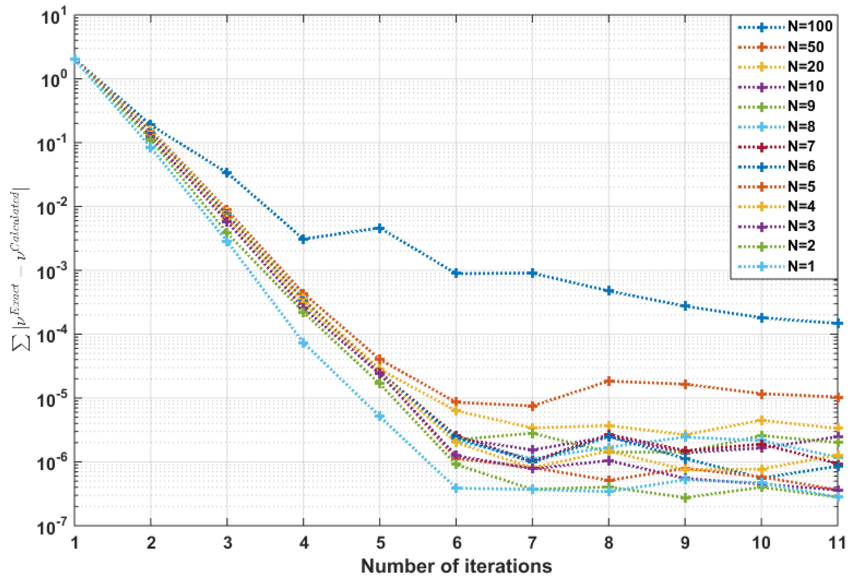
This implies that the required set can be restricted to the first few eigenvalues. In fact, when the number of input eigenvalues increases, the error also increases, which can be attributed to the approximation errors in the higher index eigenvalues (see Figure 7).

Implementation details of the steps of Algorithm 1 are as follows:

Line (Data:) 

Input eigenvalue sequence is limited to $N=10$ to get a finite sequence. Using the Magnus method on Equations (17) and (18), the truncated eigenvalue sequences ${\{{\lambda }_n\}}_1^N$, ${\{{\mu }_n\}}_1^N$ are obtained and, using Equation (20), they are combined to obtain ${\left\{{\widehat{\nu }}_n\right\}}_1^{2N}$.

Line (Result:) 

The output is a finite vector of function values: $q_0,q_1,\dots ,q_n$, where n is the number of subdivisions in the $x-$axis.

Line (1) 

Initial guess $q^{(0)}$ is set to $q\equiv 0$.

Line (2) 

By setting $q=0$ in Equations (17) and (18), the following expressions are easily obtained: ${\{u_n^{(0)}\}}_1^{\infty }={\{sin(n\pi x)\}}_1^{\infty }$, ${\{{\lambda }_n^{(0)}\}}_1^{\infty }={\{{(n\pi )}^2\}}_1^{\infty }$, ${\{v_n^{(0)}\}}_1^{\infty }={\{cos(n-1/2)\pi x\}}_1^{\infty }$, ${\{{\mu }_n^{(0)}\}}_1^{\infty }={\{{((n-1/2)\pi )}^2\}}_1^{\infty }$, ${\{w_n^{(0)}\}}_1^{\infty }={\{cos(\sqrt{{\nu }_n^{(0)}}\pi x)\}}_1^{\infty }$, ${\{{\omega }_n^{(0)}\}}_1^{\infty }={\{sin(\sqrt{{\nu }_n^{(0)}}\pi x)\}}_1^{\infty }$, ${\{{\nu }_n^{(0)}\}}_1^{\infty }={\{{\lambda }_n^{(0)}\}}_1^{\infty }\bigcup {\{{\mu }_n^{(0)}\}}_1^{\infty }$. For the rest of the algorithm, the eigenfunctions ${\left\{w_n^{(k)}(x),{\omega }_n^{(k)}(x)\right\}}_1^{2N}$ are kept fixed at ${\left\{w_n^{(0)}(x),{\omega }_n^{(0)}(x)\right\}}_1^{2N}$.

Line (3) 

The optimal while loop condition: ${\widehat{\nu }}_n\ne {\nu }_n^{(k-1)},n=1,2,\dots$ may never reach due to various errors in the numerical procedure, and is relaxed to ${\sum }_{n=1}^{2N}|{\widehat{\nu }}_n-{\nu }_n^{(k-1)}|<tol$, and/or $k<kMAX$ where $tol$ is a fixed tolerance and $kMAX$ is a maximum number of iterations.

Line (4) 

The required derivatives and integrals in Equation (24) are approximated using the Matlab built-in functions gradient() and trapz(), respectively. Furthermore, the Matlab built-in function griddedInterpolant() with linear interpolation method is used to obtain an explicit functional form of q from the set of points $q_0,q_1,\dots ,q_n$. This is necessary because, in the next step, the explicit form of q should be the input to the Magnus method (which allows evaluating $q(x)$ at an arbitrary point). Only one of the EVPs (Equation (21) or (22)), needs to be solved using the Magnus method since only the eigenvalue sequence ${\left\{{\nu }_n^{(k)}\right\}}_1^{2N}$ is needed (as the eigenfunctions are kept fixed) in the subsequent iterations.

Algorithm 1: Solving inverse SLP.

3. Results of Direct Sturm–Liouville Problems

In this section, some numerical examples of Sturm–Liouville problems of different orders are presented. Furthermore, the efficiency and accuracy of the proposed technique outlined in the previous section is investigated, numerically. Two examples are presented in the next section, illustrating the Magnus method’s usefulness in solving inverse SLPs.

Here, we made use of the MATLAB 2014 package to code the three algorithms, namely: multi-section method (Listing S1), the Magnus method for solving SLP (Listing S2), and Barcilon’s method for solving inverse SLP (Listing S3). The codes were executed on an Intel ^® Core ™ i3 CPU with power 2.40 GHz, equipped with 8 GB RAM (see Supplementary Materials).

For the numerical results (unless otherwise specified), the parameter values were: $m=100$, $n=500$, and $L=5$ where n is the number of subdivisions in the interval $[a,b]$ and m is the number of subdivisions in the interval $[{\lambda }_0,{\lambda }^{*}]$, ${\lambda }^{*}$ being the maximum eigenvalue searching, and L is the number of multisection steps used to calculate each eigenvalue in the characteristic function.

The performance of the Magnus method was measured by the absolute error $E_k$, which is defined as

$$\begin{array}{cc}\hfill E_k& =\left|{\lambda }_k^{(Exact)}-{\lambda }_k^{(Magnus)}\right|,k=1,2,\dots \hfill \end{array}$$

(26)

where ${\lambda }_k^{(Magnus)}$ indicates the kth eigenvalue obtained by the Magnus method and ${\lambda }_k^{(Exact)}$ is the kth exact eigenvalue and the relative error ${ϵ}_k$ which is defined as

$$\begin{array}{cc}\hfill {ϵ}_k& =\left|\frac{{\lambda }_k^{(Exact)}-{\lambda }_k^{(Magnus)}}{{\lambda }_k^{(Exact)}}\right|,k=1,2,\dots .\hfill \end{array}$$

(27)

There are several parameters in the Magnus method, which affect the performance and the accuracy of the method:

• eigenvalue index: k or eigenvalue: ${\lambda }_k$
• number of subdivisions in $\lambda$: m
• number of subdivisions in x: n
• number of multisection iterations: L

The performance was measured by the computation time used. Here, the Matlab function timeit() was used. timeit measures the time required to run a function by calling the specified function multiple times, and computing the median of the measurements. It provides a robust measurement of the time required for function execution and the function provides a more vigorous estimate [44]. The accuracy was measured using the absolute and relative errors as defined in Equations (26) and (27), respectively. Example 1 illustrates the affect of these variables on a SLP.

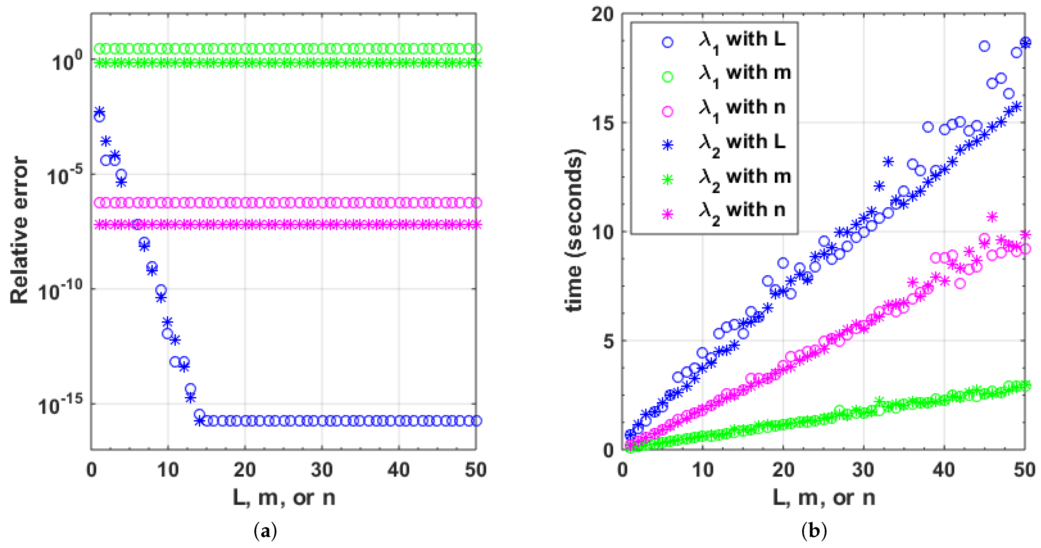
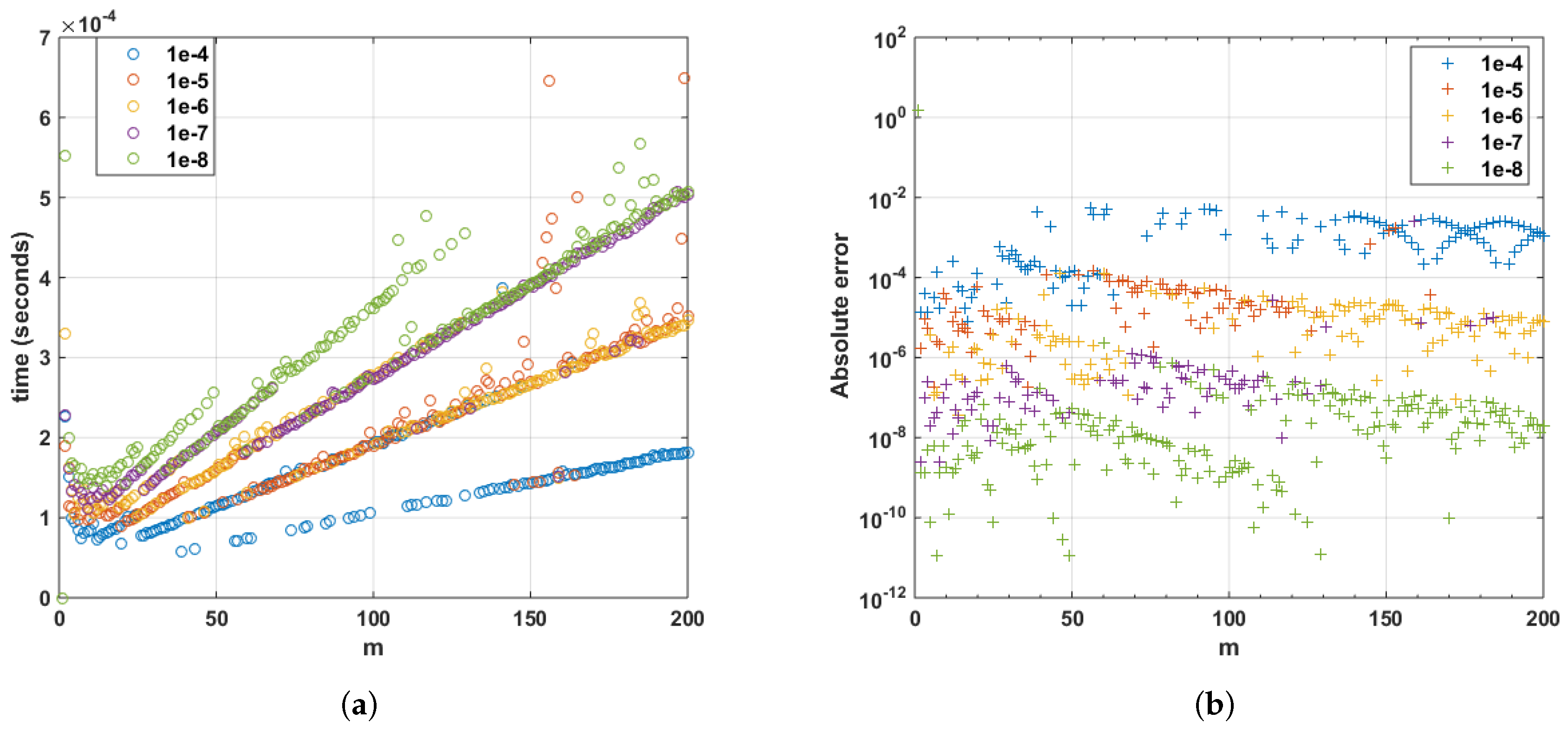
Example 1.

Consider the eigenvalue problem:

$$\begin{array}{cc}\hfill -y^{″}=\lambda y,& 0<x<1,y(0)=y(1)=0,\hfill \end{array}$$

(28)

having the exact eigenvalues ${\lambda }_k={(k\pi )}^2$, $k=1,2,\dots .$

In Figure 1a, the absolute error is increasing (as the eigenvalues are increasing quadratically), however, the relative error is (independent of λ) gradually decreasing as $\lambda \to \infty$.This shows the Magnus method’s ability to find higher index eigenvalues with less relative error. (see

Table A1. Profile summary of the slp function generated by Matlab with $m=10$, $n=10$, and $L=5$ for finding the eigenvalue in: (A) the interval $[0,10]$ for $y^{″}+\lambda y=0,y(0)=y(1)=0$; and (B) the interval $[0,2]$ for $y^{″}+{(x+0.1)}^{-2}y=\lambda y,y(0)=y(\pi )=0$. * Self time is the time spent in a function excluding the time spent in its child functions. Self time also includes overhead resulting from the process of profiling. All time values are in seconds.

Function Name	Calls	Total Time		Self Time *
		A	B	A	B
slp	1	2.442 s	2.461 s	0.028 s	0.031 s
Omega	660	2.323 s	2.292 s	0.024 s	0.030 s
R3	660	2.163 s	2.200 s	0.056 s	0.032 s
G	44,880	1.454 s	1.480 s	0.948 s	1.014 s
R2	1320	1.336 s	1.404 s	0.040 s	0.063 s
R1	3960	1.114 s	1.307 s	0.096 s	0.095 s
Q2	9240	0.843 s	0.900 s	0.140 s	0.124 s
Q3	4620	0.736 s	0.548 s	0.096 s	0.078 s
G2	17,160	0.711 s	0.653 s	0.140 s	0.110 s
G1	13,860	0.602 s	0.516 s	0.104 s	0.078 s
Q1	12,540	0.527 s	0.623 s	0.076 s	0.048 s
G3	13,860	0.481 s	0.654 s	0.096 s	0.156 s
p	44,880	0.216 s	0.171 s	0.216 s	0.171 s
w	44,880	0.180 s	0.141 s	0.180 s	0.141 s
q	44,880	0.110 s	0.155 s	0.110 s	0.155 s
expm	660	0.091 s	0.139 s	0.008 s	0.031 s
expm>PadeApproximantOfDegree	660	0.067 s	0.108 s	0.067 s	0.092 s
expm>expmchk	660	0.016 s	0.000 s	0.016 s	0.000 s
expm>getPadeCoefficients	660	0.000 s	0.016 s	0.000 s	0.016 s

in Appendix A for a detailed analysis of the code). In addition, the computation time is very slowly increasing linearly with the index of the eigenvalue (Figure 1b). As expected, accuracy and computation time increase with $m-$the number of subdivisions of λ and $L-$the number of multisection iteration steps (Figure 2). After around $L=15$, the error no longer improves, thus it is sufficient to stop at 15 iterations.

As Figure 2b shows, the computation time increases with the number of subdivisions of x: $n-$, but there is no change in the error (Figure 2a). This is obvious, since in Equation (28) all coefficient functions are constant, hence G is independent of x and the number of subdivisions n.

Example 2

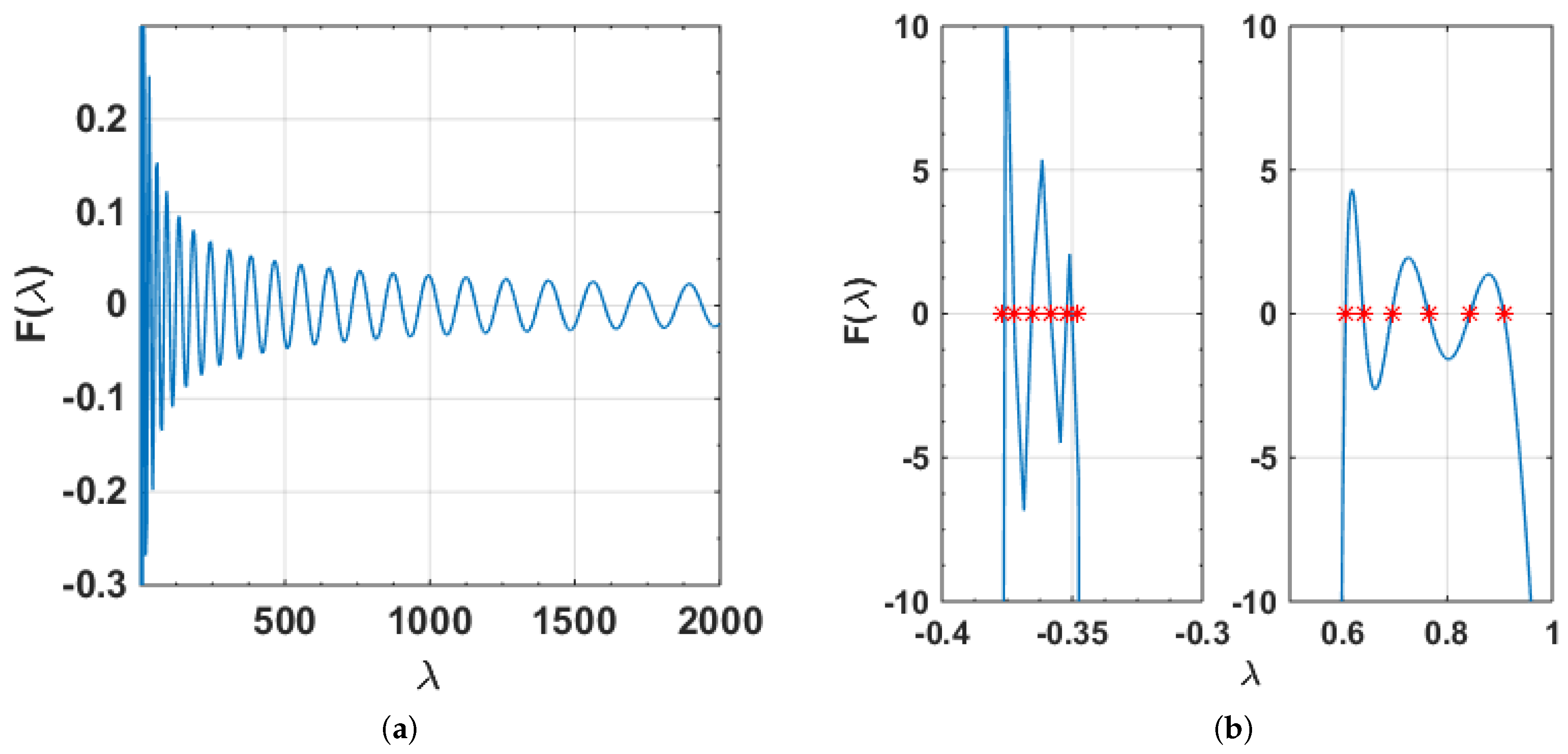
(SL Regular problem). This is an almost singular eigenvalue problem due to Paine et al. [3].

$$\begin{array}{cc}\hfill -y^{″}+{(x+0.1)}^{-2}y=\lambda y,& 0<x<\pi ,y(0)=y(\pi )=0.\hfill \end{array}$$

(29)

Table 1. First four eigenvalues of $-y^{″}+{(x+0.1)}^{-2}y=\lambda y$, $0<x<\pi$, $y(0)=y(\pi )=0$.

k	Eigenvalue
	${\mathit{\lambda }}_{\mathit{k}}$ [6], Table 4	Magnus
1	$1.5198658E+00$	$1.5198658206340E+00$
2	$4.9433098E+00$	$4.9433098197780E+00$
3	$1.0284663E+01$	$1.0284662639575E+01$
4	$1.7559958E+01$	$1.7559957737891E+01$

and

Table 2. Relative errors for the first four eigenvalues of $-y^{″}+{(x+0.1)}^{-2}y=\lambda y$, $0<x<\pi$, $y(0)=y(\pi )=0$. (Minimum relative error for each eigenvalue is in bold.)

k	Relative Error
	Magnus	FDM [3]	NM [4]	FEM [5]	MNM [6]	FEMT [7]	FEMS [7]	LGM [8]
1	$1.21E-08$	$\mathbf{0.00}\mathit{E}+\mathbf{00}$	$2.63E-06$	$1.91E-04$	$3.95E-06$	$1.32E-04$	$1.41E-03$	$2.74E-11$
2	$4.00E-09$	$8.09E-05$	$4.86E-06$	$3.03E-04$	$8.50E-06$	$2.16E-04$	$2.02E-04$	$\mathbf{2.27}\mathit{E}-\mathbf{11}$
3	$3.50E-08$	$8.75E-05$	$7.10E-06$	$3.51E-04$	$8.75E-06$	$2.78E-04$	$2.37E-04$	$\mathbf{5.26}\mathit{E}-\mathbf{11}$
4	$1.49E-08$	$9.68E-05$	$9.23E-06$	$3.59E-04$	$1.73E-05$	$3.17E-04$	$2.55E-04$	$\mathbf{1.15}\mathit{E}-\mathbf{09}$

list the first four eigenvalues of this problem and compare the relative errors with FDM ([3], Table 4), NM ([4], Table 3), FEM ([5], Table 3), MNM ([6], Table 5), FEMT and FEMS ([7], Table 2), and LGM ([8], Table 4) methods. The Magnus method exhibits good relative errors compared with the other methods.

Figure 3a shows the characteristic function for this problem. It can be seen that the roots (eigenvalues) are simple and also the eigenvalues are further apart as the index increases.

Example 3

(Singular SLP). The Magnus method is robust and can handle even singular Sturm–Liouville Problems. For example, consider the Bessel equation of order $\frac{1}{2}$ ([45], Test problem 19):

$$\begin{array}{cc}\hfill x{y}^{″}+\frac{1}{4x}y=\lambda xy,& 0<x<1,y(1)=0.\hfill \end{array}$$

(30)

Here, $p(0)=0$ and the exact eigenvalues are ${\lambda }_k={(k\pi )}^2$. The endpoint $a=0$ is singular and a limit-circle non-oscillatory (LCN) point (Note that Assumptions A3 and A4 mentioned in Section 2.1 no longer hold). Taking Friedrich’s BCs, $f=1,g=lnx$, and writing the boundary condition coefficients as:

$$\begin{array}{cc}\hfill \left(\begin{array}{cc}1& log(0)\\ 1& log(1)\end{array}\right)\left(\begin{array}{cc}y(0)& y(1)\\ y^{\prime }(0)& y^{\prime }(1)\end{array}\right)& =\left(\begin{array}{c}0\\ 0\end{array}\right)\hfill \end{array}$$

the eigenvalues can be easily obtained as: ${\lambda }_1=9.864557319999999$, ${\lambda }_2=39.458190680000001$, ${\lambda }_3=88.780786309999996,$ and so on.

Example 4.

This example—a version of the Mathieu equation—is also due to (Pryce [45], Test problem 5).

$$\begin{array}{cc}\hfill y^{″}+(cosx)y=\lambda y,& 0<x<40,y(0)=y(40)=0.\hfill \end{array}$$

(31)

Here, the lower eigenvalues form clusters of 6 (see Figure 3b). Using a sufficiently small step size (<0.004: the minimum difference between two consecutive eigenvalues) for the subdivision in $\lambda -$dimension, the Magnus method is able to find even the lower eigenvalues with an accuracy comparable to Matslise’s (see

Table 3. The first 17 eigenvalues and errors for the version of the Mathieu equation (Equation (31)) using Matslise and Magnus method.

k	Matslise [9]	Magnus	Absolute Difference
1	$-3.76845881566946E-01$	$-3.7684593940E-01$	$5.78330540124128E-08$
2	$-3.72222021386702E-01$	$-3.7222207135E-01$	$4.99632979988895E-08$
3	$-3.65517698755253E-01$	$-3.6551773700E-01$	$3.82447470359537E-08$
4	$-3.58145409533808E-01$	$-3.5814543445E-01$	$2.49161919985141E-08$
5	$-3.51818307563677E-01$	$-3.5181832065E-01$	$1.30863230252132E-08$
6	$-3.48153086495489E-01$	$-3.4815309260E-01$	$6.10451100779841E-09$
7	$6.06260772683456E-01$	$6.0626073600E-01$	$3.66834560505680E-08$
8	$6.39995069435221E-01$	$6.3999503360E-01$	$3.58352210128032E-08$
9	$6.94009291118601E-01$	$6.9400929280E-01$	$1.68139902001485E-09$
10	$7.64487943746816E-01$	$7.6448803840E-01$	$9.46531840684273E-08$
11	$8.43278584575029E-01$	$8.4327879680E-01$	$2.12224970930208E-07$
12	$9.07400354525007E-01$	$9.0740065280E-01$	$2.98274993038028E-07$
13	$1.27292510798947E+00$	$1.2729246720E+00$	$4.35989469860232E-07$
14	$1.38181949226729E+00$	$1.3818194944E+00$	$2.13271000859550E-09$
15	$1.52597349120834E+00$	$1.5259736064E+00$	$1.15191659988412E-07$
16	$1.69586866996862E+00$	$1.6958688256E+00$	$1.55631380005516E-07$
17	$1.88425137561091E+00$	$1.8842516480E+00$	$2.72389089950309E-07$

).

Example 5

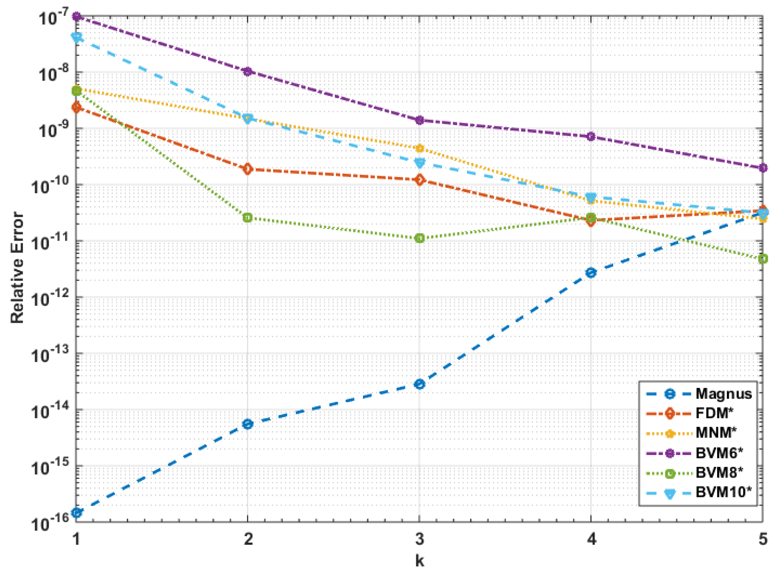
(FSLP: Simple BCs). This example is due to (Rattana and Böckmann [24], Example 1):

$$\begin{array}{cc}\hfill y^{(4)}+y& =\lambda y,y(0)=y^{″}(0)=y(1)=y^{″}(1)=0.\hfill \end{array}$$

(32)

By Schueller [46], exact eigenvalues are: ${\lambda }_k={(k\pi )}^4+1,k=1,2,\dots$.

From the results in

Table 4. The first five eigenvalues for $y^{(4)}+y=\lambda y$, $y(0)=y^{″}(0)=y(1)=y^{″}(1)=0$.

k	Eigenvalue
	${\mathit{\lambda }}_{\mathit{k}}$	Magnus
1	$9.84090910340024E+01$	$9.84090910340024E+01$
2	$1.55954545654404E+03$	$1.55954545654403E+03$
3	$7.89113637375420E+03$	$7.89113637375442E+03$
4	$2.49377273047046E+04$	$2.49377273046367E+04$
5	$6.08816818962515E+04$	$6.08816818943245E+04$

and

Table 5. The relative errors of the first five eigenvalues for $y^{(4)}+y=\lambda y$, $y(0)=y^{″}(0)=y(1)=y^{″}(1)=0$. Relative errors for all the methods except Magnus method are calculated from the eigenvalues reported in ([24], Table 5). * denotes the methods with correction terms. (Minimum relative error for each eigenvalue is in bold.)

k	Relative Error
	Magnus	FDM *	MNM *	BVM6 *	BVM8 *	BVM10 *
1	$\mathbf{1.44}\mathit{E}-\mathbf{16}$	$2.38E-09$	$5.11E-09$	$9.73E-08$	$4.71E-09$	$4.14E-08$
2	$\mathbf{5.54}\mathit{E}-\mathbf{15}$	$1.88E-10$	$1.49E-09$	$1.04E-08$	$2.57E-11$	$1.52E-09$
3	$\mathbf{2.84}\mathit{E}-\mathbf{14}$	$1.22E-10$	$4.43E-10$	$1.40E-09$	$1.10E-11$	$2.47E-10$
4	$\mathbf{2.72}\mathit{E}-\mathbf{12}$	$2.31E-11$	$5.16E-11$	$7.11E-10$	$2.60E-11$	$6.07E-11$
5	$3.17E-11$	$3.44E-11$	$2.45E-11$	$1.96E-10$	$\mathbf{4.73}\mathit{E}-\mathbf{12}$	$3.15E-11$

and Figure 4, it is clear that the Magnus method is more accurate. However, unlike the other methods, the accuracy decreases with the index of the eigenvalue due to the increasing magnitude of the eigenvalue. In contrast, for the second-order SLP using the Magnus method, the relative error decreases with the index (Figure 1a).

Example 6

(FSLP: General BCs). This example involving more general boundary conditions was taken from ([24], Example 4) to illustrate the Magnus method’s versatility.

$$\begin{array}{cc}& y^{(4)}+(sin(x)+2)y=\lambda y,\hfill \\ y(0)-y^{\prime }(0)\hfill & =0,y(0)-y^{″}(0)=0,\hfill \\ y(1)-y^{\prime }(1)\hfill & =0,y(1)-y^{″}(1)=0.\hfill \end{array}$$

(33)

As Rattana and Böckmann [24], (pp. 153) claimed, the exact eigenvalues of this problem could not be computed and there is no other method except matrix methods (MM) proposed by them to approximate the eigenvalues.

Table 6. The first five eigenvalues of FSLP in Equation (33). * Eigenvalues (except for the Magnus method) were computed using the codes provided by F. Fischer, PhD student at the Potsdam University, Germany. For each eigenvalue computed using Magnus method, the closest ones by other methods are in bold.

k	Magnus	FDM *	MNM *	BVM6 *	BVM8 *	BVM10 *
1	$3.5224017568E+00$	$3.444790E+00$	$2.604110E+00$	$\mathbf{3.522380}\mathit{E}+\mathbf{00}$	$\mathbf{3.522380}\mathit{E}+\mathbf{00}$	$\mathbf{3.522380}\mathit{E}+\mathbf{00}$
2	$5.0300125581E+02$	$5.025637E+02$	$5.017770E+02$	$5.029616E+02$	$\mathbf{5.029632}\mathit{E}+\mathbf{02}$	$5.029627E+02$
3	$3.8059852148E+03$	$3.804507E+03$	$3.804414E+03$	$3.805476E+03$	$\mathbf{3.805498}\mathit{E}+\mathbf{03}$	$3.805491E+03$
4	$1.4620083327E+04$	$1.461435E+04$	$\mathbf{1.461949}\mathit{E}+\mathbf{04}$	$1.461735E+04$	$1.461746E+04$	$1.461743E+04$
5	$3.9946254570E+04$	$3.992330E+04$	$\mathbf{3.995076}\mathit{E}+\mathbf{04}$	$3.993665E+04$	$3.993704E+04$	$3.993692E+04$

lists the first five eigenvalues of the problem and it can be seen that the values by the Magnus method are comparable with values computed by matrix methods. Figure 4 we shows that the BVM8 method with correction terms performs better than the other methods considered (except Magnus) in that example. Table 6 clearly shows that Magnus method’s values are closer to the BVM8’s values for this example.

Example 7.

This example illustrates Magnus method’s superiority over some of the other existing methods. This problem describes the free lateral vibration of a uniform clamped-hinged beam (CH) [17]:

$$\begin{array}{cc}\hfill y^{(4)}& =\lambda y,y(0)=y^{\prime }(0)=y(1)=y^{″}(1)=0.\hfill \end{array}$$

(34)

From [17], Equation (45), the eigenvalues are the solutions of the equation:

$$\begin{array}{cc}\hfill tanh\sqrt[4]{\lambda }& =tan\sqrt[4]{\lambda }.\hfill \end{array}$$

(35)

As

Table 7. The first five eigenvalues of the problem in Equation (34).

k	Eigenvalue
	${\mathit{\lambda }}_{\mathit{k}}$	Magnus
1	$2.377210675300E+02$	$2.377210675300E+02$
2	$2.496487437860E+03$	$2.496487437860E+03$
3	$1.086758221698E+04$	$1.086758221697E+04$
4	$3.178009645408E+04$	$3.178009645380E+04$
5	$7.400084934916E+04$	$7.400084934040E+04$

and

Table 8. Relative error of the first five eigenvalues for the problem in Equation (34). (Minimum relative error for each eigenvalue is in bold.)

k	Relative Error
	Magnus	CSCM [17]	ADM [16]	HAM [18]	PDQ [19]	FDQ [19]	CM [20]	CDM [22]	VIM [23]	SPSS [21]
1	$4.6E-12$	$2.4E-6$	$4.7E-12$	$\mathbf{0.0}\mathit{E}+\mathbf{00}$	$7.6E-9$	$3.2E-9$	$4.7E-12$	$2.0E-09$	$6.7E-11$	$4.6E-12$
2	$1.4E-12$	$9.8E-6$	$4.4E-12$	$4.0E-12$	$4.4E-8$	$4.8E-8$	$3.0E-12$	$7.9E-10$	$4.0E-10$	$\mathbf{1.2}\mathit{E}-\mathbf{12}$
3	$1.2E-12$	$9.3E-6$	$1.0E-06$	$\mathbf{9.2}\mathit{E}-\mathbf{13}$	$1.7E-8$	$2.2E-8$	$5.1E-12$	$2.3E-10$	$1.8E-09$	$2.1E-12$
4	$8.8E-12$	$9.3E-6$	$9.6E-03$	$\mathbf{6.0}\mathit{E}-\mathbf{12}$	$2.4E-8$	$1.7E-8$	$8.6E-09$	$2.0E-11$	$2.0E-09$	$4.2E-11$
5	$1.2E-10$	$9.3E-6$	-	$\mathbf{3.5}\mathit{E}-\mathbf{11}$	$3.0E-8$	$1.9E-8$	-	$7.5E-11$	$3.5E-09$	$2.3E-10$

point out, the Magnus method has a comparable relative error to the other methods considered (CSCM ([17], Table 4), ADM [16], HAM [18], PDQ and FDQ ([19], Table 1), CM ([20], Tables 1 and 2), CDM ([22], Table 2), VIM ([23], Table 2), and SPSS [21]) with respect to the first five eigenvalues.

More examples on Magnus methods for FSLP can be found in Mirzaei [25].

Example 8

(SSLP).

$$\begin{array}{cc}\hfill -y^{(6)}& =\lambda y,0<x<\pi ,y(0)=y^{″}(0)=y^{(4)}(0)=y(\pi )=y^{″}(\pi )=y^{(4)}(\pi )=0.\hfill \end{array}$$

(36)

This example is due to Greenberg and Marletta [29] (Problem (1)), having exact eigenvalues: ${\lambda }_k=k^6$, $k=$ 1,2, …

Again, as shown in

Table 9. Eigenvalues and relative error for the problem in Equation (36). (Minimum relative error for each eigenvalue is in bold.)

k	Eigenvalue		Relative Error
	Exact	Magnus	Magnus	Shooting [29]	ADM [30]	CP [31]	VIM [23]
1	$1.00000E+00$	$9.99999999999844E-01$	$1.56E-13$	$2.00E-07$	$\mathbf{0.00}\mathit{E}+\mathbf{00}$	$\mathbf{0.00}\mathit{E}+\mathbf{00}$	$5.50E-09$
2	$6.40000E+01$	$6.40000000000014E+01$	$2.20E-14$	$1.72E-07$	$\mathbf{0.00}\mathit{E}+\mathbf{00}$	$\mathbf{0.00}\mathit{E}+\mathbf{00}$	$7.32E-09$
3	$7.29000E+02$	$7.28999999999632E+02$	$5.05E-13$	-	$\mathbf{0.00}\mathit{E}+\mathbf{00}$	$\mathbf{0.00}\mathit{E}+\mathbf{00}$	$5.88E-09$
4	$4.09600E+03$	$4.09599999998837E+03$	$2.84E-12$	$1.71E-07$	$\mathbf{0.00}\mathit{E}+\mathbf{00}$	$\mathbf{0.00}\mathit{E}+\mathbf{00}$	$1.61E-08$
5	$1.56250E+04$	$1.56249999999687E+04$	$2.00E-12$	-	$1.28E-13$	$\mathbf{6.40}\mathit{E}-\mathbf{15}$	$2.82E-09$
6	$4.66560E+04$	$4.66559999797840E+04$	$4.33E-10$	$1.71E-07$	$1.00E-08$	$\mathbf{2.18}\mathit{E}-\mathbf{15}$	$4.62E-09$
7	$1.17649E+05$	$1.17648998941287E+05$	$9.00E-09$	-	$1.34E-04$	$\mathbf{6.50}\mathit{E}-\mathbf{11}$	$2.94E-08$
8	$2.62144E+05$	$2.62143988377187E+05$	$4.43E-08$	$1.53E-07$	$1.24E-01$	-	$\mathbf{9.50}\mathit{E}-\mathbf{09}$
9	$5.31441E+05$	$5.31440822457814E+05$	$3.34E-07$	-	-	-	$\mathbf{1.25}\mathit{E}-\mathbf{07}$
10	$1.00000E+06$	$1.00000000400001E+06$	$\mathbf{4.00}\mathit{E}-\mathbf{09}$	$1.70E-07$

, the Magnus method shows excellent accuracy with regard to this sixth-order SLP compared to other methods, namely Shooting method ([29], Table 1), ADM ([30], Table 2), CP ([31], Table 2), and VIM ([23], Table 3).

To the authors’ best knowledge, there exists no algorithms for solving eighth-order SLP in the literature. However, the proposed Magnus method can be successfully applied with literally no modification to the algorithm. Only the matrix G has to be modified using Equation (36).

Example 9

(Eighth-order Sturm–Liouville problem). Squaring the fourth-order SLP:

$$\begin{array}{cc}\hfill y^{(4)}& =\lambda y,y(0)=y^{″}(0)=y(1)=y^{″}(1)=0,\hfill \end{array}$$

(37)

with exact eigenvalues ${\lambda }_k={(k\pi )}^4,k=1,2,\dots$, the following eighth-order SLP is obtained:

$$\begin{array}{cc}\hfill y^{(8)}& ={\lambda }^{2}y,y(0)=y^{″}(0)=y^{(4)}(0)=y^{(6)}(0)=y(1)=y^{″}(1)=y^{(4)}(1)=y^{(6)}(1)=0,\hfill \end{array}$$

(38)

with exact eigenvalues ${\lambda }_k^2={(k\pi )}^8,k=$1,2, ….

The first five eigenvalues have good accuracy, although the error is steadily increasing with the index of the eigenvalue (see

Table 10. Eigenvalues and relative errors for the problem in Equation (38) using $m=100$, $n=100$, and $L=10$.

k	Eigenvalue		Relative Error
	${\mathit{\lambda }}_{\mathit{k}}$	Magnus
1	$9.48853101607057E+03$	$9.48853101607059E+03$	$1.91704005653253E-15$
2	$2.42906394011407E+06$	$2.42906394011394E+06$	$5.21434895376847E-14$
3	$6.22542519964390E+07$	$6.22542519964604E+07$	$3.43361538321867E-13$
4	$6.21840368669201E+08$	$6.21840368667400E+08$	$2.89626411740934E-12$
5	$3.70645742815257E+09$	$3.70645742800000E+09$	$4.11625897732872E-11$

). This is because the error also depends on the magnitude of the eigenvalue.

Specifically, the error in a pth-order method grows as $\mathcal{O}(h^{p+1}{\lambda }^{p/2-1})$, and thus one expects poor approximations for large eigenvalues [38].

It is clear that Magnus method has the potential to find the first eigenvalues of a SLP of arbitrary (even) order with good accuracy.

In addition, it is observed for the EVPs with constant coefficients (hence, constant and mostly sparse G matrix) the errors are smaller ($n=2$: Example 1; $n=4$: Examples 5 and 7; $n=6$: Example 8; and $n=8$: Example 9) irrespective of the order. However, when G is no longer a constant, the error is not as good even for the SLP of order two (see Example 2). This can be attributed to the matrix exponent calculation step and can be improved by using a more accurate method in place of the expm() function.

4. Results of Inverse Sturm–Liouville Problems

Example 10

(Symmetric potential). Consider the EVP

$$\begin{array}{cc}\hfill u^{″}+(\lambda -q(x))u& =0,x\in (0,1)\hfill \end{array}$$

Suppose $q(x)=cos(\pi x)$, which is symmetric and normalized. The truncated eigenvalue sequences at $N=10$, for Dirichlet boundary conditions (DDBCs): $u(0)=u(1)=0$ and Dirichlet– Neumann boundary conditions (DNBCs): $v^{\prime }(0)=v(1)=0$ are calculated using the Magnus method (using a tolerance $1E-13$), and combined into ${\left\{{\widehat{\nu }}_n\right\}}_1^{2N}$. This is the input to the algorithm. Now, using an initial guess, say $q=0$, the eigenvalue sequences for DDBCs and DNBCs are calculated again using the Magnus method and the sequence ${\left\{{\nu }_n^{(0)}\right\}}_1^{2N}$ is constructed. Then, q is updated using Equations (24) and (25). This cycle is repeated again. The iteration stops when the desired accuracy is reached.

Figure 5 and Figure 6 show the exact and reconstructed potential q and the log absolute errors in the reconstructed potential and the eigenvalue sequences, respectively. The supremum norm difference between the reconstructed q and the actual q is $8.229454025521221E-05$. It is clear that the error is larger at the end-points than in the middle. At the mid-point, $q(x)$ is 0 and, from Equation (23), this implies a minimum error (see Figure 6a). The supremum norm difference between the reconstructed eigenvalues and the actual ones is $1.302601049246732E-07$. In addition, after about 15 iterations, the differences in the two sets of eigenvalues no longer improves, and only oscillates, implying that more iterations may try to overfit (Figure 6b).

For this potential, as the number of eigenvalues increases the error also increases, due to the errors in approximating higher index eigenvalues (see Figure 7). This agrees with Aceto et al. [43] who claimed that the first eigenvalues are the most important for the reconstruction of a symmetric, zero-mean potential q, thus the required set should be restricted to the first few eigenvalues. In addition, after about six iterations, the error no longer improves, and even increases for some values of N. Thus, it is advisable to stop the iteration procedure by checking the error.

Example 11

(Non-symmetric potential). For a second example, consider $q(x)=x-0.5$, which is non-symmetric but normalized. Figure 5 and Figure 6 show the exact and reconstructed potential q and the log absolute errors in the reconstructed potential and the reconstructed eigenvalue sequence, respectively. The supremum norm difference between the reconstructed q and the actual q is 0.016647548176497. Although not as good as for the symmetric potential, this can be improved if the exact eigenvalues for the exact potential (here, we are calculating them using the Magnus method) are known. The supremum norm difference between the reconstructed eigenvalues sequence and the actual ones is 0.004796140075996. Similar to previous example, the error is larger at the end-points than in the middle (Figure 6a).

According to Andrew [15], there are three major sources of error with the inverse problem:

E4: 

attempting to compute q using only a finite (and often quite small) number of eigenvalues, even though the complete infinite set is required for the determination of q;

E5: 

only approximations of the eigenvalues are available and errors in the given eigenvalues may be especially serious for higher eigenvalues; and

E6: 

all errors in the numerical solution of the direct problem cause errors in the solution of the inverse problem.

The last one is the only error source that is affected by the choice of numerical method and which can be reduced by using a high accuracy method such as the Magnus method.

5. Discussion and Conclusions

There are several places where approximation errors occur in the Magnus method. For the direct problem, they are (see Section 2.5 also):

E1: 

truncation of the Magnus series

E2: 

calculation of multivariate integrals

E3: 

computing the matrix exponent

In the case of the inverse problem (see also Section 4) they are:

E4: 

using a finite number of eigenvalues

E5: 

using approximate eigenvalues

E6: 

errors in the direct problem

E7: 

computing the explicit form of q by an interpolation method

E8: 

approximating derivatives and integrals using numerical methods

Thus, the accumulated error would be high for the direct and inverse SLPs. For the direct SLP, we can address E1 by using a higher order Magnus method, E2 by using higher order quadrature methods, and E3 by using a more accurate method from the methods proposed by Moler and Van Loan [47]. For the inverse SLP, E4 is no longer a problem as Aceto et al. [43] argued that the first eigenvalues are the most important for the reconstruction of the unknown potential. E5 and E6 can also be reduced by reducing the errors in the direct problem (E1–E3). E8 can be eliminated by using exact derivatives and integrals when possible. Thus, it turn outs that the error in the inverse problem solely depends on the errors in the direct problem and E7 (interpolating q from a set of points).

By construction, the Magnus method leads to a global error of order $\mathcal{O}(h^p)$ if a pth-order Magnus method is applied, yet it turns out that the error also depends on the magnitude of the eigenvalue. Specifically, the error in a pth-order method grows as $\mathcal{O}(h^{p+1}{\lambda }^{p/2-1})$, and thus one expects poor approximations for larger eigenvalues [38]. This method has the disadvantage that the cost of integration, while increasing very slowly as a function of $\lambda$, wouls be $\mathcal{O}\left({\left(\begin{array}{c}2n\\ n\end{array}\right)}^2\right)$ for a problem arising from a $2n$th-order Sturm–Liouville problem [40].

The Magnus method was tested with finite interval SLPs of even orders (up to eight) along with regular and a finite singular endpoint BC, and good accuracy with regard to first few eigenvalues was obtained. One limitation of the Magnus method is that, although it is more accurate and efficient with constant coefficient BVPs irrespective of the order, when G is no longer a constant, the error is large even for the SLP of order 2. This needs to be addressed in a future work, as this would in turn effect the performance of the inverse SLP algorithm. It is an open problem whether this method can be extended to solve other types of EVPs such as different finite singular endpoints, infinite intervals, and multiple eigenvalues.

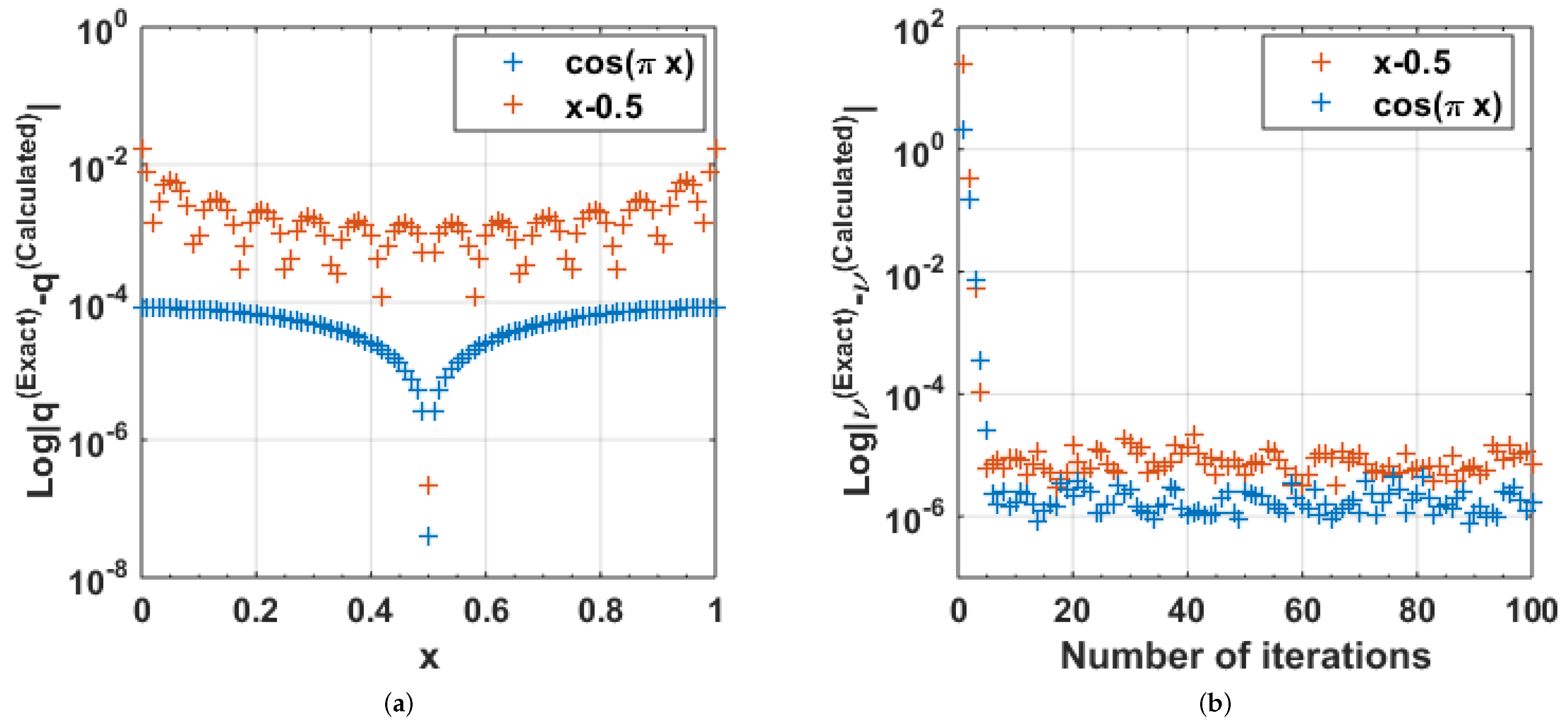
The present inverse SLP algorithm is less accurate with non-symmetric potentials, and it also should be improved to handle non-normalized, and/or non-smooth potentials. In a future work, the algorithm for inverse SLP may be modified to include general finite interval problems (i.e., problems in the domain $(a,b)$) for different sets of BCs (provided the spectra are interlaced), infinite BCS, and different classes of potential functions, such as non-smooth, discontinuous, oscillating, etc. In addition, a more suitable interpolation method for reconstructing q may be examined. Furthermore, Barcilon [26] generalized the inverse SLP algorithm presented in [14] to higher-order problems. This can be utilized in combination with Magnus method so that a direct or inverse SLP of any (even) order can be solved effectively.

In conclusion, the Magnus method is able to deal with general the kind of boundary conditions, since the boundary conditions are presented in a matrix form. Here, it is shown that the proposed technique has the ability to solve regular Sturm–Liouville problems of any even order, efficiently. By Ledoux et al. [10], a modified Magnus method can be used with Lobatto points to improve the error. Although in theory, this method can be used for solving higher order SLPs; for it to be effective in practice, the various errors in the approximation steps should be addressed adequately.

References

1. Lanczos, C. An Iteration Method for the Solution of the Eigenvalue Problem of Linear Differential and Integral Operators; United States Government Press Office: Los Angeles, CA, USA, 1950.
2. Ambarzumian, V. Über eine frage der eigenwerttheorie. Zeitschrift für Physik A Hadrons and Nuclei 1929, 53, 690–695. [Google Scholar]
3. Paine, J.W.; de Hoog, F.R.; Anderssen, R.S. On the correction of finite difference eigenvalue approximations for Sturm-Liouville problems. Computing 1981, 26, 123–139. [Google Scholar] [CrossRef]
4. Andrew, A.L.; Paine, J.W. Correction of Numerov’s eigenvalue estimates. Num. Math. 1985, 47, 289–300. [Google Scholar] [CrossRef]
5. Andrew, A.L.; Paine, J.W. Correction of finite element estimates for Sturm-Liouville eigenvalues. Num. Math. 1986, 50, 205–215. [Google Scholar] [CrossRef]
6. Vanden Berghe, G.; De Meyer, H. A modified Numerov method for higher Sturm-Liouville eigenvalues. Int. J. Comput. Math. 1990, 37, 63–77. [Google Scholar] [CrossRef]
7. Berghe, G.V.; De Meyer, H. A finite-element estimate with trigonometric hat functions for Sturm–Liouville eigenvalues. J. Comput. Appl. Math. 1994, 53, 389–396. [Google Scholar] [CrossRef]
8. Moan, P.C. Efficient Approximation of Sturm-Liouville Problems Using Lie-Group Methods; Report–DAMPT NA; Department of Applied Mathematics & Theoretical Physics, University of Cambridge: Cambridge, UK, 1998. [Google Scholar]
9. Ledoux, V.; Daele, M.V.; Berghe, G.V. MATSLISE: A MATLAB package for the numerical solution of Sturm-Liouville and Schrödinger equations. ACM Trans. Math. Softw. 2005, 31, 532–554. [Google Scholar] [CrossRef]
10. Ledoux, V.; Daele, M.V.; Berghe, G.V. Efficient numerical solution of the one-dimensional Schrodinger eigenvalue problem using Magnus integrators. IMA J. Numer. Anal. 2009, 30, 751–776. [Google Scholar] [CrossRef]
11. Atay, M.T.; Kartal, S. Computation of Eigenvalues of Sturm-Liouville Problems using Homotopy Perturbation Method. Int. J. Nonlinear Sci. Numer. Simul. 2010, 11, 105–112. [Google Scholar]
12. Freiling, G.; Yurko, V.A. Inverse Sturm-Liouville Problems and Their Applications; NOVA Science Publishers: New York, NY, USA, 2001. [Google Scholar]
13. McLaughlin, J.R. Analytical methods for recovering coefficients in differential equations from spectral data. SIAM Rev. 1986, 28, 53–72. [Google Scholar] [CrossRef]
14. Barcilon, V. Iterative solution of the inverse Sturm-Liouville problem. J. Math. Phys. 1974, 15, 429–436. [Google Scholar] [CrossRef]
15. Andrew, A.L. Numerov’s method for inverse Sturm–Liouville problems. Inverse Probl. 2005, 21, 223–238. [Google Scholar] [CrossRef]
16. Attili, B.S.; Lesnic, D. An efficient method for computing eigenelements of Sturm-Liouville fourth-order boundary value problems. Appl. Math. Comput. 2006, 182, 1247–1254. [Google Scholar] [CrossRef]
17. Mai-Duy, N. An effective spectral collocation method for the direct solution of high-order ODEs. Commun. Numer. Methods Eng. 2006, 22, 627–642. [Google Scholar] [CrossRef]
18. Abbasbandy, S.; Shirzadi, A. A new application of the homotopy analysis method: Solving the Sturm–Liouville problems. Commun. Nonlinear Sci. Numer. Simul. 2011, 16, 112–126. [Google Scholar] [CrossRef]
19. Yücel, U.; Boubaker, K. Differential quadrature method (DQM) and Boubaker polynomials expansion scheme (BPES) for efficient computation of the eigenvalues of fourth-order Sturm–Liouville problems. Appl. Math. Model. 2012, 36, 158–167. [Google Scholar] [CrossRef]
20. El-Gamel, M.; Sameeh, M. An Efficient Technique for Finding the Eigenvalues of Fourth-Order Sturm-Liouville Problems. Appl. Math. 2012, 3, 920–925. [Google Scholar] [CrossRef] [Green Version]
21. Khmelnytskaya, K.V.; Kravchenko, V.V.; Baldenebro-Obeso, J.A. Spectral parameter power series for fourth-order Sturm–Liouville problems. Appl. Math. Comput. 2012, 219, 3610–3624. [Google Scholar] [CrossRef]
22. Taher, A.S.; Malek, A.; Momeni-Masuleh, S. Chebyshev differentiation matrices for efficient computation of the eigenvalues of fourth-order Sturm–Liouville problems. Appl. Math. Model. 2013, 37, 4634–4642. [Google Scholar] [CrossRef]
23. Taher, A.H.S.; Malek, A. An efficient algorithm for solving high order Sturm-Liouville problems using variational iteration method. Fixed Point Theory 2013, 14, 193–210. [Google Scholar]
24. Rattana, A.; Böckmann, C. Matrix methods for computing eigenvalues of Sturm–Liouville problems of order four. J. Comput. Appl. Math. 2013, 249, 144–156. [Google Scholar] [CrossRef]
25. Mirzaei, H. Computing the eigenvalues of fourth order Sturm-Liouville problems with Lie Group method. Iran. J. Numer. Anal. Optim. 2017, 7, 1–12. [Google Scholar] [CrossRef]
26. Barcilon, V. On the solution of inverse eigenvalue problems of high orders. Geophys. J. Int. 1974, 39, 143–154. [Google Scholar] [CrossRef]
27. McLaughlin, J.R. An Inverse Eigenvalue Problem of Order Four. SIAM J. Math. Anal. 1976, 7, 646–661. [Google Scholar] [CrossRef]
28. McLaughlin, J.R. An Inverse Eigenvalue Problem of Order Four—An Infinite Case. SIAM J. Math. Anal. 1978, 9, 395–413. [Google Scholar] [CrossRef]
29. Greenberg, L.; Marletta, M. Oscillation Theory and Numerical Solution of Sixth Order Sturm–Liouville Problems. SIAM J. Numer. Anal. 1998, 35, 2070–2098. [Google Scholar] [CrossRef]
30. Lesnic, D.; Attili, B.S. An efficient method for sixth-order Sturm-Liouville problems. Int. J. Sci. Technol. 2007, 2, 109–114. [Google Scholar]
31. Allame, M.; Ghasemi, H.; Kajani, M.T. An appropriate method for eigenvalues approximation of sixth-order Sturm-Liouville problems by using integral operation matrix over the Chebyshev polynomials. In AIP Conference Proceedings; AIP Publishing: College Park, MD, USA, 2015; Volume 1684, p. 090001. [Google Scholar]
32. Zhang, Z. How Many Numerical Eigenvalues Can We Trust? J. Sci. Comput. 2015, 65, 455–466. [Google Scholar] [CrossRef]
33. Barcilon, V. On the uniqueness of inverse eigenvalue problems. Geophys. J. R. Astron. Soc. 1974, 38, 287–298. [Google Scholar] [CrossRef]
34. McLaughlin, J.R.; Rundell, W. A uniqueness theorem for an inverse Sturm–Liouville problem. J. Math. Phys. 1987, 28, 1471–1472. [Google Scholar] [CrossRef]
35. Bailey, P.B.; Gordon, M.K.; Shampine, L.F. Automatic solution of the Sturm-Liouville problem. ACM Trans. Math. Softw. 1978, 4, 193–208. [Google Scholar] [CrossRef]
36. Lie, S. Theorie der Transformationsgruppen; Ripol Classic: Moscow, Russia, 1970; Volume 1. [Google Scholar]
37. Iserles, A.; Norsett, S. On the solution of linear differential equations in Lie groups. Philos. Trans. R. Soc. Lond. Ser. A Math. Phys. Eng. Sci. 1999, 357, 983–1019. [Google Scholar] [CrossRef] [Green Version]
38. Blanes, S.; Casas, F.; Oteo, J.; Ros, J. The Magnus expansion and some of its applications. Phys. Rep. 2009, 470, 151–238. [Google Scholar] [CrossRef] [Green Version]
39. Magnus, W. On the exponential solution of differential equations for a linear operator. Commun. Pure Appl. Math. 1954, 7, 649–673. [Google Scholar] [CrossRef]
40. Jódar, L.; Marletta, M. Solving ODEs arising from non-selfadjoint Hamiltonian eigenproblems. Adv. Comput. Math. 2000, 13, 231–256. [Google Scholar] [CrossRef]
41. Iserles, A. Magnus expansions and beyond. Comb. Phys. 2008, 539, 171–186. [Google Scholar] [CrossRef]
42. Borg, G. Eine Umkehrung der Sturm-Liouvilleschen Eigenwertaufgabe: Bestimmung der Differentialgleichung durch die Eigenwerte. Acta Math. 1946, 78, 1–96. [Google Scholar] [CrossRef]
43. Aceto, L.; Ghelardoni, P.; Magherini, C. Boundary value methods for the reconstruction of Sturm–Liouville potentials. Appl. Math. Comput. 2012, 219, 2960–2974. [Google Scholar] [CrossRef]
44. McKeeman, B. MATLAB Performance Measurement—File Exchange—MATLAB Central; MathWorks: Natick, MA, USA, 2008. [Google Scholar]
45. Pryce, J.D. A Test Package for Sturm-Liouville Solvers. ACM Trans. Math. Softw. 1999, 25, 21–57. [Google Scholar] [CrossRef]
46. Schueller, A. Eigenvalue Asymptotics for Self-Adjoint, Fourth-Order, Ordinary Differential Operators. Ph.D. Thesis, University of Kentucky, Lexington, KY, USA, 1997. [Google Scholar]
47. Moler, C.; Van Loan, C. Nineteen dubious ways to compute the exponential of a matrix, twenty-five years later. SIAM Rev. 2003, 45, 3–49. [Google Scholar] [CrossRef]
Figure 1. (a) Log absolute error (red) and log relative error (magenta); and (b) computing time (in seconds) (blue circles) and linear trend line (orange dashed line) for the first 100 eigenvalues using Magnus method for the problem y = λ y , 0 < x < 1 , y ( 0 ) = y ( 1 ) = 0 .
Mathematics 07 00544 g001
Figure 2. (a) Relative error; and (b) computation time (in seconds) for the first two eigenvalues λ 1 (∘) and λ 2 ( * ) of the problem y = λ y , 0 < x < 1 , y ( 0 ) = y ( 1 ) = 0 using Magnus method: for m = 10 , L = 5 , and n = 1 , , 50 (magenta); for n = 10 , m = 10 , and L = 1 , , 50 (blue); for n = 10 , L = 1 , and m = 1 , , 50 (green).
Mathematics 07 00544 g002
Figure 3. (a) Characteristic function of y + ( x + 0.1 ) 2 y = λ y , 0 < x < π , y ( 0 ) = y ( π ) = 0 . (b) Parts of the characteristic equation (blue) and first 12 eigenvalues (red) for the version of Mathieu Equation (31).
Mathematics 07 00544 g003
Figure 4. Log relative error of the first five eigenvalues of the problem in Equation (32).
Mathematics 07 00544 g004
Figure 5. Exact and reconstructed potentials q ( x ) = cos ( π x ) and q ( x ) = x 0.5 .
Mathematics 07 00544 g005
Figure 6. (a) Log absolute error in the reconstructed q; and (b) log absolute error sum of the difference of the eigenvalue sequences { ν ^ n } and { ν n ( k 1 ) } for reconstructing the potentials q ( x ) = cos ( π x ) (blue) and q ( x ) = x 0.5 (red).
Mathematics 07 00544 g006
Figure 7. Sum of the absolute errors in the reconstructed eigenvalues: | ν E x a c t ν C a l c u l a t e d | using the Magnus method vs. the iteration number, using eigenvalue sets of sizes N = 1 , , 10 , 20 , 50 , 100 for reconstructing the potential q ( x ) = cos ( π x ) .
Mathematics 07 00544 g007