1. Introduction
Economic model predictive control (EMPC) that integrates optimization of process economics with process control has attracted significant attention over the last decade (e.g., [
1,
2,
3]). Unlike the traditional two-layered real-time optimization (RTO) that continuously optimizes process set-points in the upper level and applies a tracking model predictive controller or a proportional-integral-derivative controller in the lower layer, EMPC operates the system in a time-varying fashion (off steady-state) by dynamically optimizing an economic cost function accounting for stability constraints in one layer. Many research works have been done on EMPC in terms of closed-loop stability, economic optimality, model uncertainty and process operational safety (e.g., [
4,
5,
6]). However, to achieve a desired closed-loop performance under EMPC, it is acknowledged that a reliable process model that can predict the future state evolution accurately is a key requirement. To that end, multiple linear state-space models have been used within EMPC to capture the nonlinear dynamics in the operating region in [
7]. Additionally, a well-conditioned polynomial nonlinear state-space model has been used in [
8] to approximate the actual (first-principles) nonlinear process model (normally substituting of the actual nonlinear process) for EMPC. Given the recent interest in machine learning modeling and particularly its usage in solving nonlinear regression problems ([
9,
10]), in this work, we will derive a nonlinear data-driven process model for EMPC by taking advantage of machine learning techniques.
Machine learning has been widely used in a variety of engineering problems such as classification, pattern recognition, and numerical prediction. Among machine learning methods, neural networks have shown great success in regression problems. With the rapid development of neural network libraries and application programming interfaces e.g., Tensorflow [
11], Caffe [
12], Keras [
13], etc.), building a neural network has presently become intuitive and straightforward. Additionally, neural network-based modeling outperforms other data-driven modeling methods due to its ability to implicitly detect complex nonlinearities and the availability of multiple training algorithms ([
14]). Neural network has undergone several phases in which different theoretical approaches led to increasing understanding of its power and limitations. For example, in the 1980s, the first RNN (i.e., Hopfield networks) was created for pattern recognition ([
15]). At that time, implementing a neural network with many layers for complex systems was a technical challenge [
16]. Subsequently, deep learning was proposed to alleviate the problems of vanishing gradient in RNNs, which provided a new perspective to the machine learning field [
17]. Compared to feedfoward neural networks, RNN is able to memorize previous information in the network and thus, can be applied to model a nonlinear dynamical system from time-series data. However, since the majority of research is focused on validating the identified system, it is not clear how RNN models can be incorporated in EMPC with guaranteed closed-loop stability.
In addition, ensemble learning, a machine learning paradigm that trains multiple models for the same problem, is gaining increasing attention in recent years ([
18,
19]). By taking advantage of multiple learning algorithms or various training datasets, ensemble learning provides better predictive performance than a single machine learning model. However, the consequent challenge for implementations of ensemble regression models in process control is how to solve the ensemble of RNNs efficiently and in a timely fashion. Although reducing the computation time of neural network training process is always an important research topic in machine learning community, process engineers are more concerned about the real-time implementation of neural networks in process control systems. To address computational implementation issues, parallel computing ([
20]) is employed to solve multiple RNN models simultaneously in EMPC.
Motivated by the above, a Lyapunov-based EMPC method using an ensemble of RNN models is developed in this work. Specifically, in
Section 2, the notation, the class of nonlinear systems considered and the stabilizability assumptions are introduced. In
Section 3, the class of RNN models and the learning algorithm are provided. Then, ensemble learning is used to obtain multiple RNN models based on a
k-fold cross validation, while parallel computing is used to improve computational efficiency. Subsequently, in
Section 4, the Lyapunov-based EMPC that incorporates an RNN ensemble is formulated to guarantee the boundedness of the state in the closed-loop stability region accounting for sufficiently small modeling error, sampling time and bounded disturbances. In the last section, the proposed LEMPC method is applied to a chemical process example to demonstrate its guaranteed closed-loop stability and economic optimality properties.
3. Recurrent Neural Network
In this work, we develop a nonlinear recurrent neural network (RNN) model with the following form:
where
is the RNN state vector and
is the manipulated input vector.
is a vector of both the network state
and the input
u, where
is the nonlinear activation function (e.g., a sigmoid function
).
A is a diagonal matrix, i.e.,
, and
is a coefficient matrix
with
,
.
and
are constants, where
is assumed to be positive such that each state
is bounded-input bounded-state stable.
is the weight connecting the
jth input to the
ith neuron where
and
. Since the RNN model of Equation (
4) is affine in the manipulated inputs
u, the RNN model can also be represented in a similar form of Equation (
1) by
, where
and
are derived from coefficients
A and
in Equation (
4). Similarly,
and
are assumed to be sufficiently smooth vector and matrix functions of dimensions
and
, respectively.
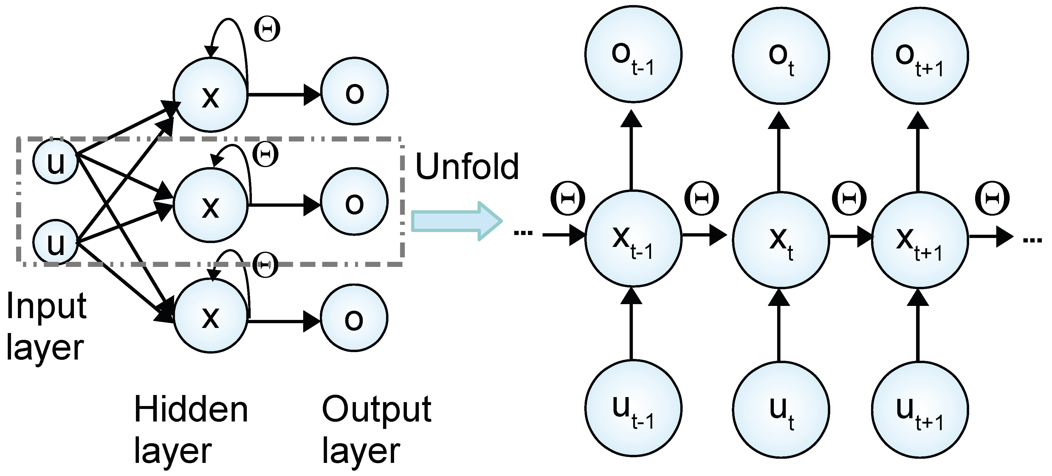
It is shown in
Figure 1 that RNNs possess a certain type of memory by introducing feedback loops in the hidden layer such that the states information derived from earlier inputs remains in the network. Additionally, if we unfold one of the RNN states in time as shown in
Figure 1, the manipulated input vector
and the previous state vector
are fed into the current state
with the weight matrix
, where
,
, and
are all internal states of an RNN model.
Due to the capability of capturing nonlinear dynamic behavior and the universal approximation theorem ([
22,
23]) demonstrating that the RNN model with sufficient neurons is able to approximate any dynamic nonlinear system on compact subsets of the state-space for finite time, the RNN model of Equation (
4) is used to approximate the continuous-time nonlinear system of Equation (
1) in this work.
3.1. RNN Learning Algorithm
The RNN learning algorithm is developed to obtain the optimal weight matrix
, under which the modeling error between the nominal system of Equation (
1) (i.e.,
) and the the RNN model of Equation (
4) is minimized. The modeling error
under
is assumed to be nonzero since the obtained RNN model may not perfectly approximate the nominal system of Equation (
1) due to insufficient number of nodes or layers. Additionally, the modeling error
is bounded (i.e.,
,
) since the RNN model of Equation (
4) is developed based on the dataset generated within
where
and
are bounded. The weight vector
of the RNN model of Equation (
4) is also bounded by
, with
to prevent the weights from drifting to infinity. Throughout the manuscript, we will use
to represent the state of the nonlinear system of Equation (
1) and
to represent the state of the RNN model of Equation (
4).
According to the definition of the modeling error
, the nominal system of Equation (
1) (i.e.,
) can be written in the following form:
where the optimal weight vector
is obtained as follows:
where
is the number of data samples used for training. Consider the state error
. Based on Equations (
4) and (
5), the time-derivative of the state error is derived as follows:
where
is the error between the current weight vector
and the unknown optimal weight vector
. The weight vector
is updated by the following equation:
where the learning rate
is a positive real number. Based on the learning law of Equation (
8), the following theorem is established to demonstrate that the state error
e remains bounded and is constrained by the modeling error
.
Theorem 1. Consider the RNN model of Equation (4) with the weights updating law of Equation (8). In the presence of a nonzero modeling error ν, the state error and the weight error are bounded, and there exist and such that the following inequality holds: Proof. We first define a Lyapunov function
and prove the boundedness of
and
by showing that
is bounded. Specifically, using Equations (
7) and (
8) and the fact that
, the time-derivative of
is first derived as follows:
In the presence of modeling error
, it is observed that
does not hold for all times. Therefore, let
and
, where
represents the maximum eigenvalue of
. The following inequality is further derived based on Equation (
10):
Since the weight vector is bounded by
, it is derived that
. According to the definitions of
and
, it follows that
. Therefore, for all
,
holds. This implies that
is bounded, and thus,
and
are bounded as well. Additionally, from Equation (
10), it is readily shown that the following equations hold:
From Equation (
12),
is obtained as follows:
where
is the minimum value of
,
. Let
and
. The following inequality is derived:
The above inequality shows that the state error
e is bounded and is proportional to the modeling error
between the RNN model of Equation (
4) and the nominal system of Equation (
1) (i.e.,
). Furthermore, if there exists a constant
such that
is bounded (i.e.,
), then it follows that
. Therefore,
converges to zero asymptotically since
is a uniformly continuous function implied by the boundedness of its derivative
. □
3.2. Ensemble of RNN Models
In this section, an RNN model is initially developed to approximate the nonlinear system of Equation (
1) within an operating region. Based on that, the ensemble learning using the aforementioned RNN learning algorithm is used with a
k-fold cross validation to improve prediction accuracy of RNN models.
3.2.1. Development of RNN Models
The development of RNN models consists of two steps: data generation and training process. In general, the dataset for training an RNN model is a collection of sampled data from industrial processes, laboratory experiments, or simulations of a given system. There are many high-quality training datasets, for example, the collection of databases from the UCI Machine Learning Repository [
24] that is widely used by the researchers in machine learning community. In this work, we use the simulation data of the nominal system of Equation (
1) (i.e.,
) as the training and validation datasets for the RNN model of Equation (
4). Specifically, to generate the dataset that captures the system dynamics for
and
, open-loop simulations are first conducted for initial conditions
with the constrained input vector
. It should be mentioned that the continuous system of Equation (
1) is simulated in a sample-and-hold fashion (i.e., the input is a piecewise constant function, i.e.,
,
, where
and
is the sampling period). Then, the nominal system of Equation (
1) is integrated via explicit Euler method with a sufficiently small integration time step
. The dataset is generated with the following steps: (1) The targeted region
and the range of inputs
are first discretized with sufficiently small intervals. (2) Open-loop simulations of the nominal system of Equation (
1) are performed in a sample-and-hold fashion with various initial states
and inputs
to obtain a large number of state trajectories for a fixed length of time to sweep over all the values that
can take. It is noted that data points are collected at every integration time step
instead of every sampling step
to obtain intermediate states as many as possible in order to approximate a continuous system of Equation (
1). (3) Then, the obtained state trajectories are separated into many time-series data samples with the length of
, which represents the prediction period for RNN models. In other words, the RNN model is developed to predict future states over
, where all the data points between
and
are treated as the internal states of the RNN model with the time interval of
(i.e., the time interval between two consecutive states
and
for the unfolded RNN shown in
Figure 1 is equal to
). (4) The dataset is partitioned into training, validation and testing datasets.
Next, the RNN model is developed based on the dataset generated from open-loop simulations via an application program interface (API), i.e., Keras ([
13]). To guarantee that the RNN model of Equation (
4) achieves good performance in a neighborhood around the origin and has the same equilibrium point as the nonlinear system of Equation (
1), the modeling error is further required to be bounded by
during the training process. Before starting an RNN training process, the number of layers and nodes used, the optimizer, and the type of loss function need to be specified at the beginning. Specifically, in our work, the number of layers and nodes for RNNs are determined through a grid search and the adaptive moment estimation method (i.e., Adam in Keras) is used as RNN optimizer. The loss function is the mean absolute percentage error between predicted states
and actual states
x from training data. Additionally, to prevent RNNs from over-training, the early stopping criteria is employed to terminate the training process before the maximum number of epochs is reached if the following two conditions are satisfied: (1) The modeling error is below its threshold. (2) The performance on the validation dataset stops improving.
Remark 2. It is noted that original data samples from open-loop simulations are shortened to a fixed length, , in the step 3 of data generation above. Through this data preprocessing step, the dataset is applicable for developing an RNN with the prediction period , which is chosen to be an integer multiple of the sampling period Δ such that the RNN model of Equation (4) is able to predict future states for at least one sampling period. One of the advantages of introducing step 2 and step 3 is that a new dataset can be conveniently generated for an RNN with a different prediction period while the original dataset in step 2 only needs to be created once. Remark 3. Unlike feedforward neural networks (FNN) that take state measurement and manipulated inputs at time to predict the state at only, RNNs use all the intermediate states between and to predict the state trajectory over this prediction period. In other words, all the internal states with the time step are used as one of the inputs (the other one is the manipulated input u) to the RNN (shown in Figure 1) over during the training process. Therefore, besides the final predicted state , all the internal states before can be predicted and exported (if needed) by RNNs. Additionally, it is important to mention that since the time interval for RNN internal states is chosen to be the sufficiently small integration time step that is used to simulate the continuous-time nonlinear system of Equation (1), the obtained RNN model can be regarded as a good representation for the continuous-time RNN model of Equation (4). Remark 4. Data quality plays an important role in data-driven modeling techniques including RNN modeling. In case a good RNN model is initially not available due to poor data quality, the RNN model can be improved via on-line update through real-time process state measurements. Additionally, if the real-time process measurements are of poor quality, for example, noisy measurements, a data preprocessing step can be employed before training an RNN. Overall, creating a good dataset remains an important issue in RNN modeling; in the chemical reactor example in Section 5 the data is generated from open-loop simulations. Remark 5. The RNN models considered in our work involve the use of nonlinear terms in the dynamic model (this can be thought of as a nonlinear process gain , multiplying the input), which allows capturing gain sign change in the different regions in the operating state-space if it occurs. This issue does not occur in the operating region of the chemical reactor example considered in Section 5. The reader may refer to [25] for an approach to neural network modeling that captures gain change. 3.2.2. Ensemble Learning
Ensemble learning is a machine learning process that combines multiple learning algorithms to obtain better prediction performance ([
26]) in terms of reduced variability and improved generalization performance. The reasons that ensemble regression models are able to improve prediction performance are given in [
10,
26]. In this work, homogeneous ensemble regression models are constructed following the RNN learning algorithm in
Section 3.1 and a
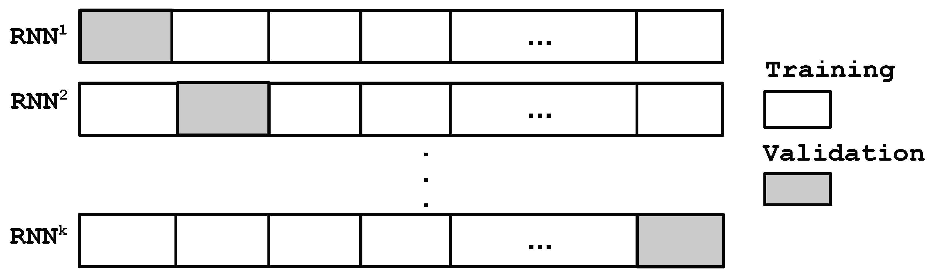
k-fold cross validation. Specifically, as shown in
Figure 2, the dataset is initially separated into
k folds with the same size, where
folds are used for training and the remaining one is used for validation. By choosing a different subset as the validation dataset every time, a total number of
k different RNNs can be obtained. Subsequently, the final prediction results of an ensemble of RNN models is calculated using the stacking method that averages the predictions of multiple RNN models. It is noted that besides the stacking method, other ensemble-based algorithms such as Boosting and Bagging [
19] can also be applied to improve the overall prediction performance within the targeted operating region.
3.2.3. Parallel Computing
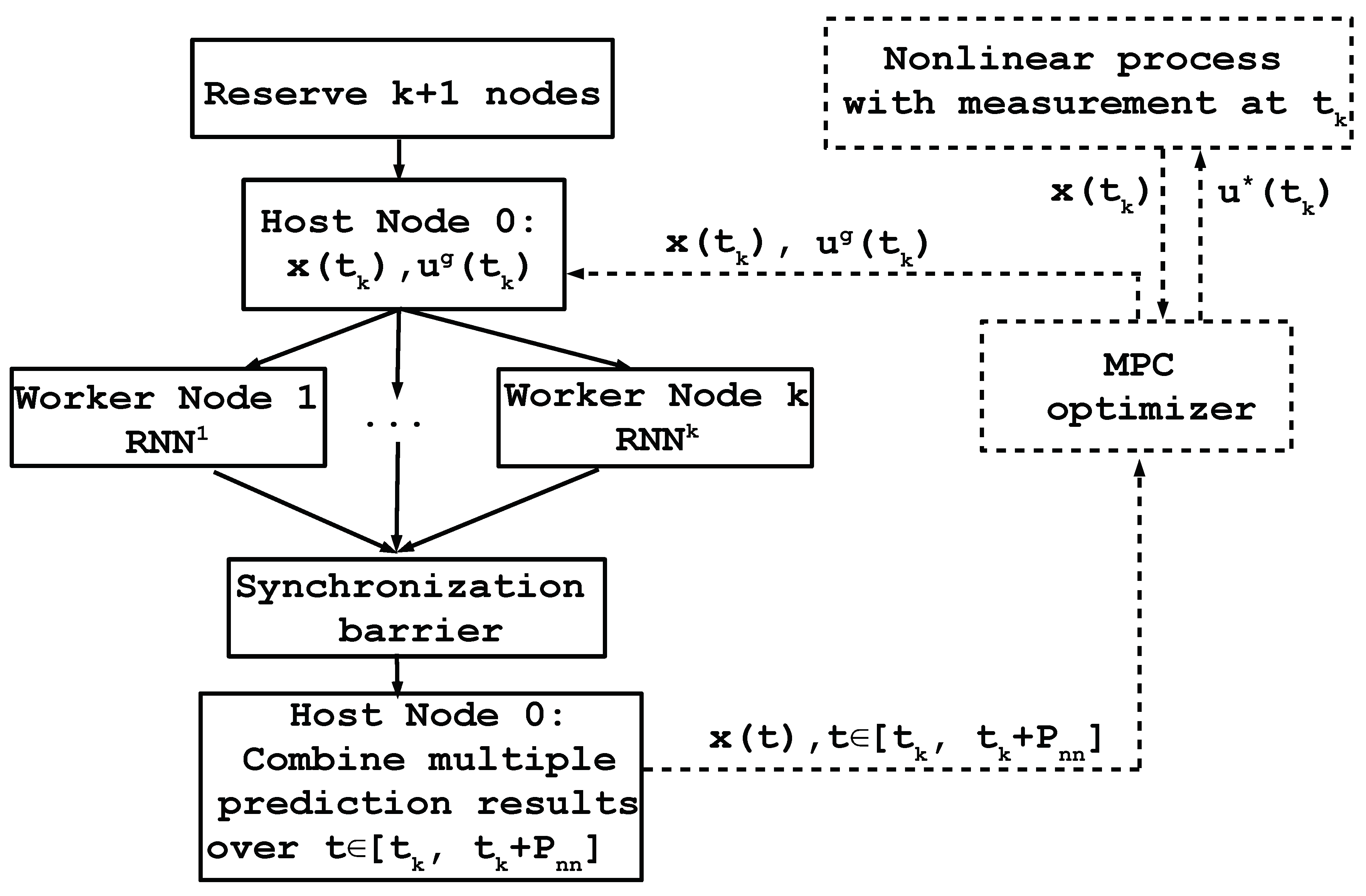
Parallel computing is a type of computation in which the execution of multiple processes or of the computational tasks are carried out simultaneously. Since the final prediction results in ensemble learning are obtained by combining the results of individual RNN models that are independent from each other, the computational tasks for all RNN models can be operated in parallel to improve computational efficiency. The algorithm for parallel computation of an ensemble of
k RNN models is shown in
Figure 3. The blocks on the left demonstrate the state prediction using parallel computing and the dashed blocks on the right represent the actual nonlinear system of Equation (
1) and the model-based controller that will be discussed in the next section. Specifically, we first reserve
nodes, where node 0 is the host node and the rest are worker nodes. The host node is used to exchange information while the worker nodes are mainly used for computation. Each worker node is assigned with a corresponding RNN model for prediction. At time
, the model-based controller receives the state measurement
and sends it to the host node 0 along with the manipulated inputs
(i.e., the guess of control actions over the prediction horizon). The host node broadcasts
and
to all worker nodes such that all RNN models share the same input vector. Prediction of RNN models are carried out in all worker nodes simultaneously. It is noted that a synchronization barrier is placed before the ensemble combiner in node 0 to ensure that all the computation tasks in worker nodes are completed. Lastly, the host node combines prediction results from multiple RNN models to obtain predicted states over
and sends them to the model-based controller. The optimal control actions
is calculated by the optimizer solver in model-based controller by taking various guesses of control actions
, and will be sent to the nonlinear process of Equation (
1) to be applied for the next sampling period. The above process is repeated as the horizon of the nonlinear process of Equation (
1) is rolled one sampling period forward each time.
5. Application to a Chemical Process Example
A chemical process example is used to illustrate the application of LEMPC using an ensemble of RNN models, under which the state of the closed-loop system is maintained within the stability region in state-space for all times. We consider a well-mixed, non-isothermal continuous stirred tank reactor (CSTR), in which an irreversible second-order exothermic reaction takes place. Specifically, the reaction transforms a reactant
A to a product
B (
). The inlet temperature, the inlet concentration of
A, and the feed volumetric flow rate of the reactor are
,
and
F, respectively. Additionally, the CSTR is equipped with a heating jacket to supply or remove heat at a rate
Q. The following material and energy balance equations are used to represent the CSTR dynamic model:
where
V is the volume of the reacting liquid in the reactor,
is the reactant
A concentration in the reactor,
Q is the heat input rate and
T is the temperature of the reactor. The feed volumetric flow rate and temperature are
F and
, respectively. The feed concentration of reactant
A is
. The reacting liquid has a constant heat capacity of
and density of
.
is the pre-exponential constant,
is the enthalpy of reaction,
R is the ideal gas constant, and
E is the activation energy. Process parameter values are listed in
Table 1.
The CSTR is initially operated at the unstable steady-state , and . In this example, the two manipulated inputs are the heat input rate, , and the inlet concentration of species A, , respectively. Additionally, the manipulated inputs are subject to the following constraints: and . The states and the inputs of the system of Equation (33) are represented by and , respectively. Therefore, the unstable steady-state of the system of Equation (33) is at the origin of the state-space, (i.e., ).
The control objective of the LEMPC of Equation (19) is to maximize the production rate of
B in the CSTR by manipulating the inlet concentration
and the heat input rate
, while maintaining the closed-loop state trajectories in the stability region
for all times under LEMPC. The objective function of the LEMPC optimizes the production rate of
B as follows:
To simulate the dynamic model of Equation (33) numerically, the explicit Euler method is used with an integration time step of
. The Python module of the IPOPT software package [
27], named PyIpopt, is used to solve the nonlinear optimization problem of the LEMPC of Equation (19) with a sampling period
. Additionally, a Message Passing Interface (MPI) for the Python programming language, named
MPI4Py ([
28]), is incorporated in the LEMPC optimization problem to execute multiple RNN predictions of Equation (
19b) concurrently in independent computing processes.
Extensive open-loop simulations for the CSTR system of Equation (33) are initially conducted to generate the dataset for RNN models. The control Lyapunov function
is designed with the following positive definite
P matrix:
Two hidden recurrent layers consisting of 96 and 64 recurrent units, respectively, are used in the RNN model. Additionally, a 10-fold cross validation are used to construct an ensemble of RNN models for the LEMPC of Equation (19). The closed-loop stability region
with
and a subset
with
for the CSTR system are characterized based on the obtained RNN models and the stabilizing controller
. To demonstrate the effectiveness of the proposed LEMPC of Equation (19), a linear state-space model (i.e.,
with
and
) is also identified following the system identification method in [
29], and is added into the following performance comparison under the ensemble of RNN models and the first-principles model of Equation (33).
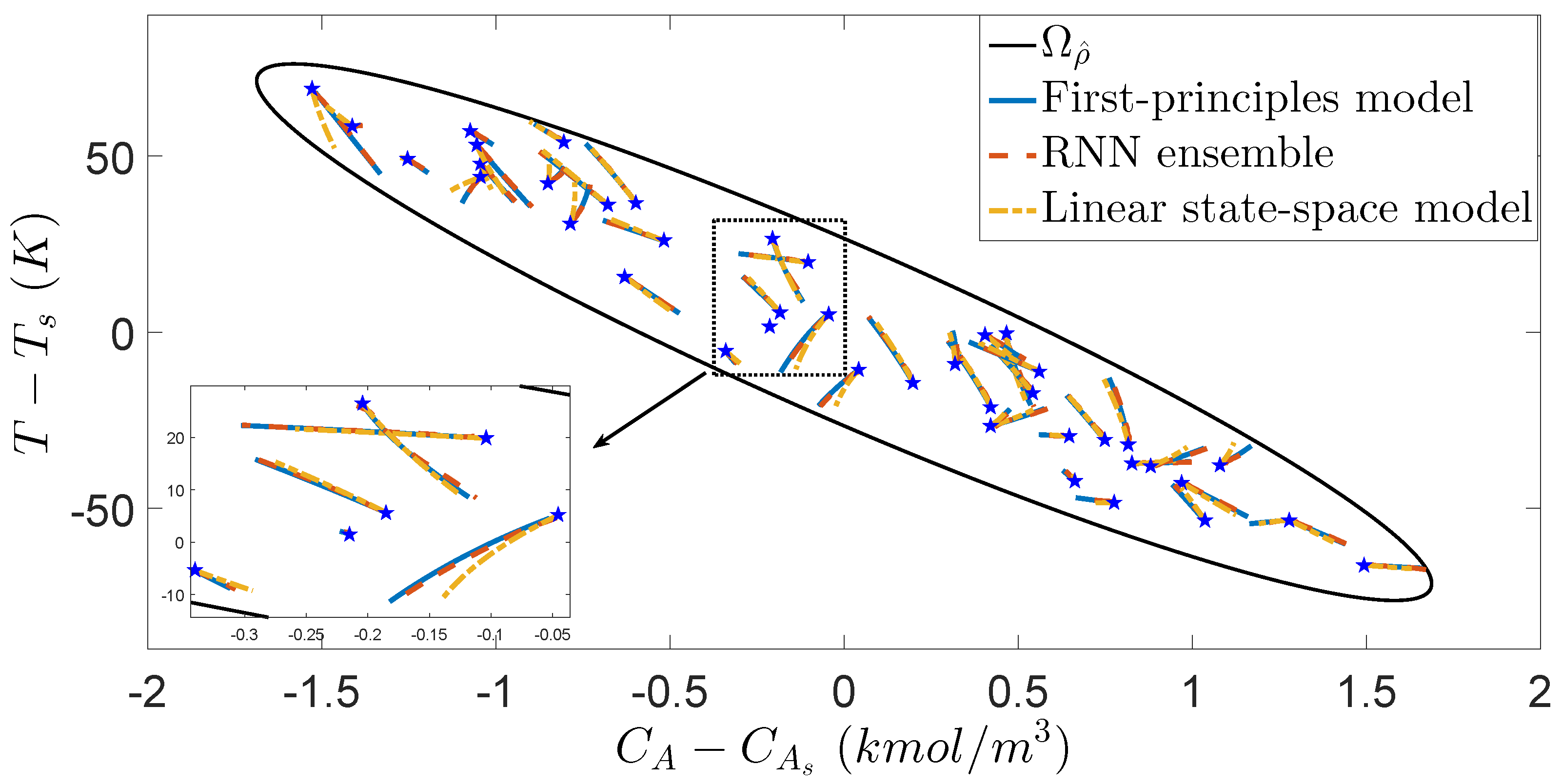
The open-loop simulation studies are first carried out for the first-principles model of Equation (33), an RNN model ensemble, and the linear state-space model, respectively. The optimal number of RNN models used in the ensemble is determined to be five from extensive simulation tests due to its best performance in terms of closeness to the trajectories under the first-principles model. As shown in
Figure 5, starting from various initial conditions in
, the state trajectories under the RNN model ensemble almost overlap those under the first-principles model using the same input sequences, while the state trajectories under the linear state-space model show considerable deviation, especially in the top and bottom regions of
. From
Figure 5, it is demonstrated that the RNN model ensemble is a good representation for the first-principles model of Equation (33) in that it successfully captures the CSTR nonlinear dynamics everywhere in
.
Subsequently, the closed-loop simulation of the nominal CSTR system (i.e.,
) under the first-principles model of Equation (33), the ensemble of RNN models, and the linear state-space model, respectively, are shown in
Figure 6. The following material constraint is used in the LEMPC of Equation (19) to make the averaged reactant material available within the entire operating period
to be its steady-state value,
(i.e., the averaged reactant material in deviation form,
, is equal to 0).
In
Figure 6, it is shown that for the initial condition (0,0), the state trajectory under the ensemble of RNN models is close to that under the first-principles model, and both state trajectories are bounded in
in the absence of disturbances. However, it is observed that the state trajectory under the linear state-space model ultimately leaves
due to its large model mismatch. This implies that a more conservative set
needs to be characterized for the state spaced model to guarantee the boundedness of state in the stability region
.
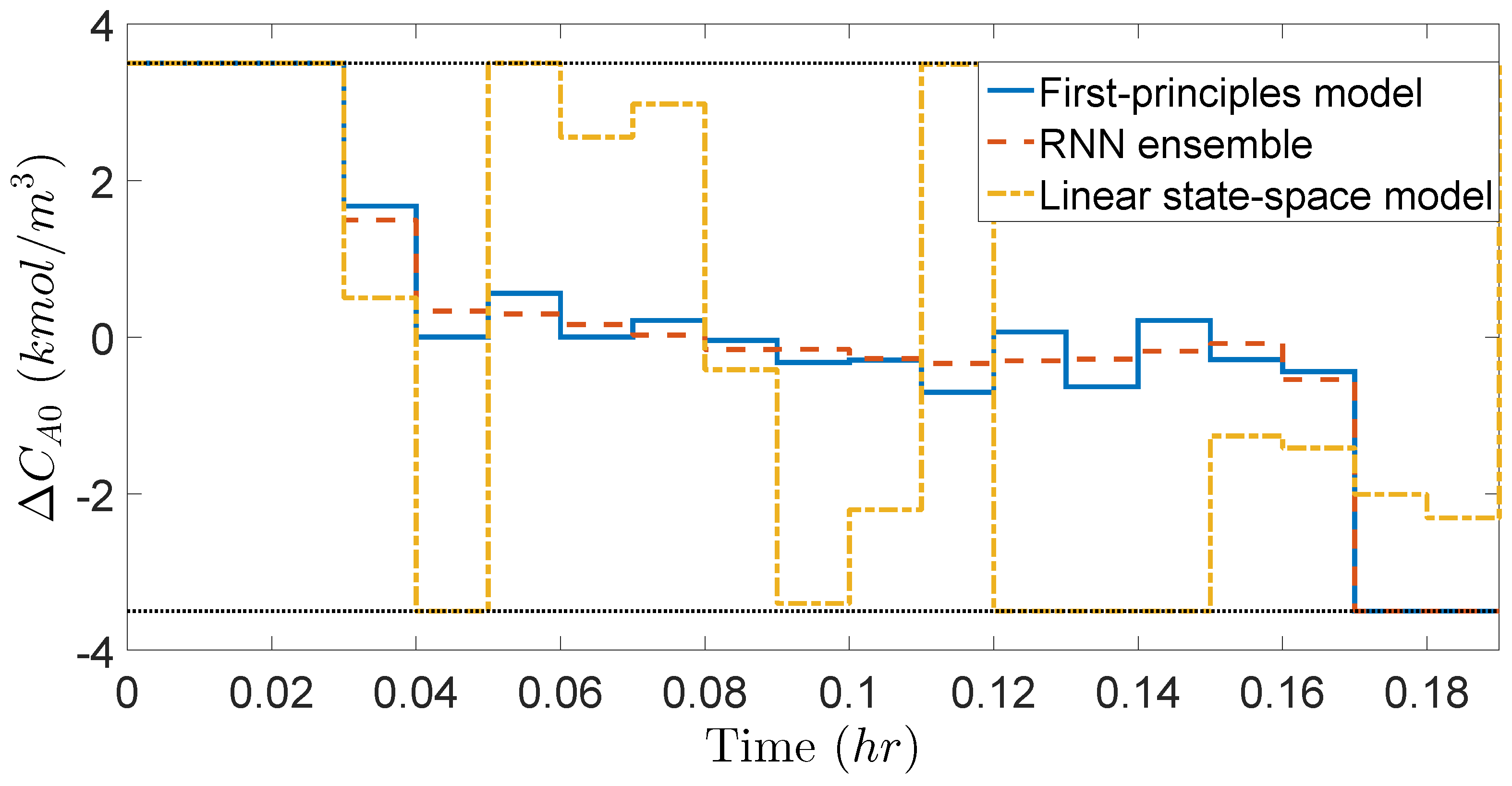
Additionally,
Figure 7 and
Figure 8 show the manipulated inputs profiles in deviation from the steady-state values. It is shown that the manipulated inputs are bounded within the input constraints for all times. Moreover, the material constraint of Equation (
36) is satisfied as it is shown in
Figure 7 that the LEMPC using the first-principles model and the RNN model ensemble both consume the maximum allowable
at the first few sampling steps, and thus have to lower the consumption of
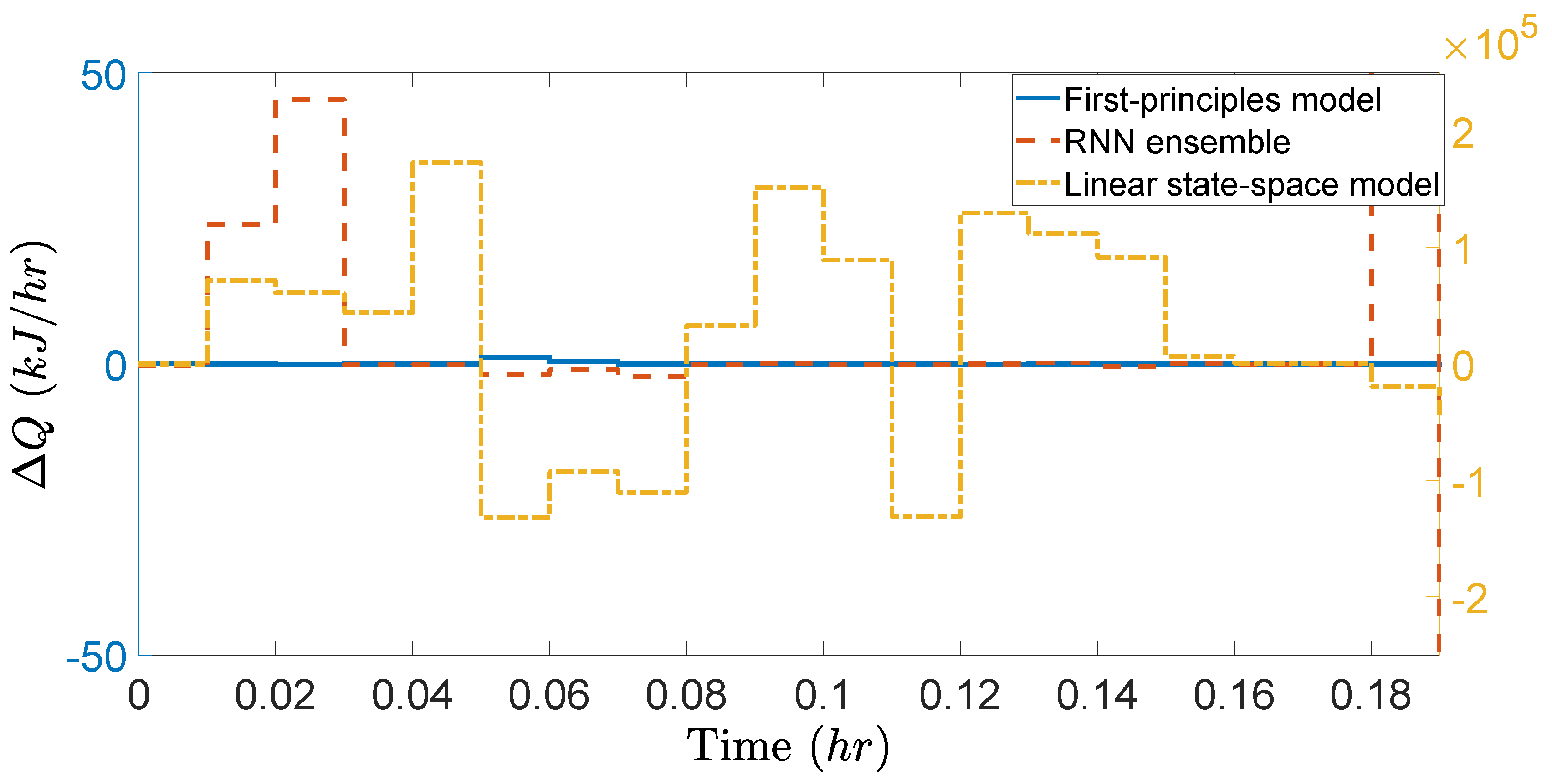
near the end of operating period. The LEMPC using the linear state-space model also satisfies the material constraint, but shows persistent oscillation due to model mismatch. Additionally, in
Figure 8, it is shown that the consumption of
under the RNN ensemble is close to that under the first-principles model (both correspond to left
y-axis) since their closed-loop trajectories shown in
Figure 6 are similar. However,
shows large oscillation under the LEMPC using the linear state-space model (right
y-axis) since the closed-loop trajectory in
Figure 6 leaves
, and thus, the contractive constraint of Equation (
19f) is activated frequently.
To demonstrate that the closed-loop system under LEMPC achieves high process economics than the steady-state operation using the same amount reactant , we calculate the accumulated economic benefits over the entire operating period = 0.2 h, which are , , and for the steady-state operation, the LEMPC under an ensemble of RNN models, and the LEMPC under the first-principles model, respectively. Therefore, it is demonstrated that both closed-loop stability and economic optimality are achieved under the proposed LEMPC using an ensemble of RNN models.


