Abstract
We obtain a list of simple classes of singularities of function germs with respect to the quasi m-boundary equivalence relation, with . The results obtained in this paper are a natural extension of Zakalyukin’s work on the new non-standard equivalent relation. In spite of the rather artificial nature of the definitions, the quasi relations have very natural applications in symplectic geometry. In particular, they are used to classify singularities of Lagrangian projections equipped with a submanifold. The main method that is used in the classification is the standard Moser’s homotopy technique. In addition, we adopt the version of Arnold’s spectral sequence method, which is described in Lemma 2. Our main results are Theorem 4 on the classification of simple quasi classes, and Theorem 5 on the classification of Lagrangian submanifolds with smooth varieties. The brief description of the main results is given in the next section.
MSC:
58K05.58K40.53A15
1. Introduction
In [1], Vladimir Zakalyukin classified function germs with respect to a new non-standard equivalence relation, which he named quasi boundary equivalence. The aim of the relation is to preserve only the positions of critical points of functions defined on a space along a smooth hypersurface. Using Zakalyukin’s idea, a similar quasi equivalence relation was introduced in which case the smooth hypersurface was replaced by an arbitrary one, called a border, in particular, when the border is a cylinder over a corner (a union of two transversal intersecting smooth hypersurfaces) or a cuspidal edge, as considered in [2,3], respectively. In the present paper, we study an even more general setting and consider an arbitrary algebraic variety of any dimension, which will be called a semi-border, and the respective relation will be named quasi semi-border equivalence. In the definition of the quasi border equivalence relation in [3], it was assumed that the border was stratified set and the stratification satisfied the Whitney Condition A. Therefore, in many cases, we will be able to establish similar results to that in [1,2,3] for semi-borders that satisfy such conditions. In particular, two function germs are pseudo semi-border equivalent, if there is a diffeomorphism acting as a change of variables, taking one germ to the other and satisfying the following condition: if one of these functions has a critical point at the semi-borders, then its image (or respectively the inverse image) also belongs to the semi-borders. After a natural modification, this equivalence relation behaves well when functions depend on parameters. The modified definition is called quasi semi-border equivalence.
As an example, we generalize the results in [1] and classify quasi simple function germs , in local coordinates , on semi-borders being submanifolds of codimension . Therefore, We will set , and the quasi semi-border equivalence will be also called the quasi m-boundary.
The quasi singularities have very natural applications related to singularities of Lagrangian projections (mappings). In fact, Arnold’s classical boundary class of functions, which depends on n parameters, corresponds to projection of a pair consisting of an n dimensional Lagrangian submanifold and a regular submanifold of dimension that intersects the first component transversally in complementary directions [4]. The quasi equivalence relation keeps information only on one Lagrangian submanifold of the pair and on its intersection with the second component. Therefore, the new relation is an appropriate model for applications when we deal with the notion of a Lagrangian submanifold with a smooth boundary. Therefore, we will discuss in the current paper the connection between the obtained simple classes and the singularities of Lagrangian projections in the presence of a submanifold of codimension m via the quasi semi-border miniversal deformation of a function germ , which can be constructed in the standard way.
The technique of the classification, described in Lemma 2, is valid for smooth function germs, and it is an important tool for reduction to the normal form. In fact, this lemma completes Arnold’s description, which is given for power series only, and it can be proven by induction on function germs of the Newton order of at least via similar methods to the standard ones, given in Sections 12.5–12.17 of [5]. Therefore, it is useful in cases not covered by the technique of Chapter 12 of [5], such as the case when the principal part is quasi homogeneous of specific degree d with indices corresponding to fixed coordinates, while basic fields, which are tangent to the semi-border, are not quasi homogeneous.
The paper is organized as follows. In Section 2, we introduce the main definitions of the pseudo and quasi semi-border equivalence relations, and also, we obtain auxiliary results on the quasi reduction for arbitrary semi-borders. In Section 3, we obtain the classifications of simple quasi m-boundary germs, described in the following:
Theorem 1.
Let be a simple germ with respect to the quasi m-boundary equivalence relation. Then, f is stably quasi m-boundary equivalent to one of the following simple classes:
| Notation | Normal Form | Restrictions | Codimension |
| – | |||
| – | |||
| – | |||
In Section 4, we discuss the main application of the quasi equivalence, and we describe the classifications of Lagrangian projections with a submanifold of codimension , in the following:
Theorem 2.
- 1.
- A pair , consisting of a Lagrangian submanifold and a semi-border, is stable if and only if its arbitrary generating family is versal with respect to the quasi semi-border equivalence and up to the addition of functions in parameters.
- 2.
- Let be a pair of a stable and simple Lagrangian submanifold with an m-boundary. Then, it is symplectically equivalent to the projection determined by a generating family that is a quasi m-boundary versal deformation of one of the classes from the above theorem with respect to the quasi m-border equivalence and up to the addition of functions in parameters.
Finally, in Section 5, we give a detailed discussion and conclusions, including the contribution of the paper and possible further applications.
2. Pseudo and Quasi Semi-Border Equivalence Relations
Consider a coordinate space with an algebraic variety in it. The variety will be called a semi-border, and it will usually be a cylinder; we therefore split the coordinates on into , which accommodate cylindrical directions for and in which the equations of are written. Sometimes, the notation will be used for the whole set of coordinates on , if the distinction between x and y is not significant.
We consider germs of functions , in local coordinates w as above. We denote by the ring of all such germs at the origin and by the maximal ideal in
Definition 1.
[3] Two functions are called pseudo semi-border equivalent if there exists a diffeomorphism such that , and if a critical point c of the function belongs to the border Γ, then also belongs to Γ, and vice versa, if c is a critical point of and belongs to Γ, then also belongs to Γ.
A similar definition can be introduced for germs of functions.
Remark 1.
- 1.
- The general statements below are valid for certain types of varieties. In particular, the variety Γ should be a stratified set, satisfying the Whitney Condition A. In addition, it is assumed in Definition 1 that if a critical point c is contained in a certain stratum of Γ, then its image must be contained in the same stratum. This means that the diffeomorphism does not need to preserve the variety, but it needs to shift the critical points along the components of the variety.
- 2.
- The pseudo semi-border equivalence will be just called the pseudo border if the variety is a hypersurface.
- 3.
- In contrast to the standard equivalence relation, the pseudo semi-border equivalence is not a group action due to the constraints on the set of admissible diffeomorphisms.
Definition 2.
[4] A vector field ζ on is said to be logarithmic for the germ if, when considered as a derivation , we have for all where and . The -module of such vector fields is denoted by , that is:
and it is called the stationary algebra of .
Remark 2.
If , then ζ preserves Γ and, hence, is tangent to it. Moreover, is the Lie algebra of the group of diffeomorphisms of preserving .
Assume a smooth family of function germs are pseudo semi-border equivalent to the function germ , with respect to a smooth family of germs of diffeomorphisms such that and . If we differentiate this relation with respect to t, we get the homological equation:
where all and the components of the vector field are evaluated at . Moreover, if we denote by the radical of the gradient ideal of the function , then following [1,2,3,6], we have:
Lemma 1.
The components of satisfy the following:
where .
Remark 3.
- 1.
- The details of the proof of Lemma 1 can be found in [6].
- 2.
- If for a given function in Equation (1), we can find a decomposition in the right side form, then the vector field in the -space can be integrated to generate the phase flow . Of course, we need to be sure that the germs of diffeomorphisms are defined on some neighborhood of the base point. This is usually achieved if the vector field vanishes at the base point. This method is called Moser’s homotopy method.
- 3.
- Due to the bad behavior of the radical of an ideal depending on a parameter (see [3]), we will put extra constraints on the pseudo equivalence relation. In particular, we exchange by the ideal in the equivalence definition. The new relation, described explicitly in the following definition, will be called the quasi semi-border equivalence.
Definition 3.
Two functions will be called quasi semi-border equivalent if they are pseudo semi-border equivalent and there are a family of functions and a piece-wise smooth family of diffeomorphisms both depending continuously on parameter such that the following are satisfied:
- 1.
- ,
- 2.
- , and
- 3.
- the components of the vector field generating on each segment of smoothness have the forms:
Remark 4.
- 1.
- Each one of the vector fields and their phase flow will be called admissible with respect to the family .
- 2.
- The tangent space to the quasi semi-border equivalence class of f, denoted by , has the following description:
Due to the inclusion , where is the gradient ideal of f, we have:
Property 1.
A function germ f has a finite codimension with respect to the quasi semi-border equivalence if and only if f has a finite codimension with respect to the right equivalence.
Property 2.
If a function germ f has a finite (right) multiplicity for any semi-border, then f has finite quasi semi-border multiplicity. In other words, the quasi semi-border tangent space has finite codimension over in the space of all germs.
Let be the gradient ideal of f. As f has a finite right multiplicity, then its local algebra , for some smooth functions , is finitely generated over .
This means that for any function germ , there is a decomposition of the form:
where are constants and are smooth function germs.
Now, for any , we can write:
This yields:
Notice that the square of the gradient ideal belongs to the quasi semi-border tangent space . Therefore, we see that
where . This completes the proof.
Definition 4.
Two function germs are stably quasi semi-border equivalent if they become quasi equivalent after the addition of nondegenerate quadratic forms in a suitable number of the variables .
Analogous to [5], a function germ is called simple with respect to the quasi semi-border equivalence if its neighborhood contains only a finite number of quasi classes.
For an arbitrary semi-border , the quasi classification of function germs with critical points lying outside coincides with the standard classes , and . Furthermore, the definition implies that all functions with non-critical points are equivalent. Therefore, we classify only the remaining case of function germs having critical base points on the strata of the semi-border.
2.1. Basic Techniques of the Classification
Moser’s homotopy method is the main tool that will be used to establish quasi semi-border equivalence between function germs. In addition, we will be using the following technique, which is similar to Lemma 8.1 in [2] and Lemma 2.10 in [3]. It will be used to establish quasi semi-border equivalence between function germs.
Consider a fixed and convenient Newton diagram . Denote by the ideals of function germs of the Newton order of at least with the appropriate scaling factor and . Then, equips with the Newton filtration and such that [5].
Let be a decomposition of a function germ f into its principal part of the Newton degree N and higher order terms . We assume that has a finite codimension with respect to the right equivalence.
Lemma 2.
Consider a monomial basis of the linear space . Let be all its elements of Newton degrees higher than N.
Suppose that for any :
- 1.
- There is an admissible vector field for , that is,such that:where and
- 2.
- Moreover, for any and any , the expression:belongs to .Then, any germ is quasi semi-border equivalent to a germ where .
Remark 5.
The quasi reduction of functions with the Newton principal part of infinite right equivalence codimension can be treated using the standard Arnold’s approaches.
2.2. Prenormal Forms of Quasi Classes
In many cases we can find a prenormal for a function germ with respect to the quasi equivalence for an arbitrary semi-borders. In fact, all results in the current subsection are analogous to the ones described for borders in [3], since their proofs depend only on the square of the gradient ideal of the function.
Let be a function germ of the form
where is a quadratic form in x and and .
Lemma 3.
Let be a function germ at the origin. Assume is a non-degenerate quadratic form in local coordinates x only. Then, f is quasi semi-border equivalent to where Moreover, if f is a germ in local coordinates x only, then f is quasi semi-border equivalent to .
Proof.
Note that the gradient ideal of f coincides with the maximal ideal in . Therefore, the admissible vector fields are those with components vanishing at the origin. It follows that the phase flows generated by such fields are all families of diffeomorphisms that preserve the origin. Hence, the Lemma can be proven using the standard Morse lemma. ☐
Denote by the restriction of f on . Let r and be the rank of the second differential and at the origin, respectively, and set .
Lemma 4.
(Stabilization) The function germ is quasi semi-border equivalent to a germ , where and . For quasi semi-border equivalent germs f, the respective reduced germs g are quasi semi-border equivalent.
Assume is a function germ having an isolated critical point at the origin, and let be its gradient ideal. Then,
Lemma 5.
The germ f is quasi semi-border equivalent to where , for each on the condition that the rank r of the second differential is constant.
Suppose that s is a non-negative integer, satisfying the constraint . Let , where with and be a quadratic form in x only. Then, Lemmas 4 and 5 infer the following.
Lemma 6.
The function germ is quasi semi-border equivalent to . Moreover, two germs f and g are quasi semi-border equivalent if the corresponding reduced germs and are quasi semi-border equivalent.
Remark 6.
The proofs of Lemma 4, Lemma 5, and Lemma 6 are identical to those of Lemma 2.13, Lemma 2.14, and Lemma 2.15 in [3], respectively, replacing the coordinates by . In fact, the admissible vector fields that are used in the proofs there are independent of the -module of vector fields preserving the cuspidal edge and depend only on the gradient ideal of a family of functions.
Lemmas 3 and 6 imply the following.
Lemma 7.
Let be a function germ with an isolated critical point at the origin, and let be the corank of the second differential at the origin. Then, f is quasi stably semi-border equivalent to one of the following germs.
| Notation | Normal Form | Restrictions | |
| 0 | |||
| 1 | , | ||
| , | |||
| , | |||
| , , | |||
| , |
3. Classifications of Simple Functions
We start this section by recalling the classification of simple singularities with respect to the quasi boundary equivalence relation from [1]. After that, we classify simple quasi semi-border singularities when is a submanifold of codimension m, which will be also called the m-boundary, and we set where (The cases when and are shown in Figure 1b and Figure 2a respectively) giving details of the proofs of the main results.
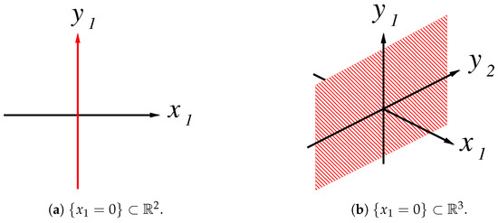
Figure 1.
The one-boundary.
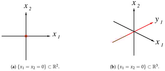
Figure 2.
The two-boundary.
Remark 7.
- 1.
- The case when the semi-border is a smooth hypersurface () was discussed in [1].
- 2.
- The quasi semi-border equivalence will be also called the quasi m-boundary for the respective type of .
- 3.
- All results are given for permutations of and .
3.1. Simple Quasi Boundary
The classification of simple quasi boundary singularities is described in the following.
Theorem 3.
[1] On the boundary , any simple quasi boundary singularity class is a class of the stabilization of one of the following two-variable germs:
| Notation | Normal Form | Restrictions | Codimension |
| k | |||
Remark 8.
- 1.
- The classes can be written in the form , and hence, it can be included in the series as
- 2.
- Corank one germs are either simple, hence they are quasi boundary equivalent to one of the germs in the above theorem, or they belong to a subset of infinite codimension in the space of all germs.
- 3.
- All germs with the quadratic part of corank greater than one are non-simple.
- 4.
- The uni-modal class is the only fencing singularity that is adjacent to .
- 5.
- The graph of low codimension adjacencies is as follows:
3.2. Simple Quasi m-Boundary Classes
Up to permutations of the coordinates , classification of simple quasi m-boundary singularities is described in the following.
Theorem 4.
Let be a simple germ with respect to the quasi m-boundary equivalence relation. Then, f is stably quasi m-boundary equivalent to one of the following simple classes:
| Notation | Normal Form | Restrictions | Codimension |
| – | |||
| – | |||
| – | |||
Remark 9.
- 1.
- In Theorem 4, .
- 2.
- The classes can be written equivalently in the forms , and hence, they can be included in the series as , where .
- 3.
- The graph of adjacencies of simple quasi m-boundary classes in low codimension is as follows:Furthermore,where , with and . Moreover, if , then:
- 4.
- The fencing class with respect to the quasi two-boundary equivalence relation is a stabilization of the following:
Notation Class Restrictions Codimension 10 11 12
To prove Theorem 4, we use the results of Section 2.2 and the following auxiliary results.
We start by describing the stationary algebra of .
Property 3.
If , then ζ has the following formula:
Proof.
The formulas are obtained by direct calculations, using Definition 2. ☐
Corollary 1.
The tangent space to the quasi semi-border equivalence class of the germ f has the following description:
Lemma 8.
The classifications of function germs in the local coordinates x only with respect to the quasi m-boundary and the standard right equivalence relations coincide.
Proof.
Indeed, if f is a function germ with a critical point at the origin in the local coordinates x only, then coincides with the ideal generated by i= 1,2,…,m over , that is Notice that vector fields with components from are all vector fields vanishing at the origin. Therefore, any family of diffeomorphisms preserving the origin is admissible, and hence, the result follows. ☐
Moreover, for an arbitrary semi-border, we have the following.
Lemma 9.
Let where in a non-degenerate quadratic form in x only and , . Then, f is quasi semi-border equivalent to:
Proof.
By Lemma 8, we can use the standard right equivalence and the versality theorem to obtain a prenormal form of with respect to the quasi semi-border equivalence. Notice that the germ f can be considered as a deformation depending on a parameter with variables x. On the other hand, Lemma 3 implies that we may write:
Set , and notice that coincide with the square of the gradient ideal of . By the versality theorem, we may consider the germ:
where are constants, as a mini-versal deformation of . This means that is induced from , and hence, f can be reduced to the form:
where and , as required. ☐
Finally, we have:
Lemma 10.
If or and f is stably m-boundary equivalent to either
, where , , , or
where , ,
then f is non-simple with respect to the quasi m-boundary equivalence relation.
Proof.
Suppose that . Then, Lemma 6 implies that f is stably m-boundary equivalent to one of the following:
0. , where , , or
1. , where , , , or
2. , where , , , or
3. , where , .
Consider the germ . By Lemma 8, we see that is non-simple.
In the next case, consider the germ . Note that deforms to:
According to Lemma 6, is stably m-boundary equivalent to , where and , which we have already shown to be non-simple. By a similar argument, we can show that is adjacent to and is adjacent to , and hence, the result follows.
The remaining cases of function germs with are adjacent to a function germ having . Therefore, they must be non-simple.
Now, let and f be stably m-boundary equivalent . Then, up to permutations of the coordinates , the germ can be reduced to the form , where , . The quadratic and cubic terms in forma subspace of dimension less than the dimension of the space of all quadratic and cubic forms in the variables x and . This means that the germ is non-simple. Finally, the germ is adjacent to , which we have already shown to be non-simple, and hence, the result follows. ☐
Proof of Theorem 4
Lemma 6 implies that any function germ is quasi m-boundary to a germ of the form , where is a quadratic form in x only and . We distinguish the following.
- If f is a function germ in x only, then Lemma 8 implies that f is quasi m-boundary equivalent to , where , and g belongs to one of Arnold’s simple classes .
- Let . Then, Lemma 7 and Lemma 10 imply that f is simple if is the non-degenerate quadratic form and , in which case, by Lemma 9, f is stably quasi m-boundary equivalent to where and . Considering the lowest non-zero terms in and , and using Lemma 2, one can easily show that is reduced to one of the following forms:
- , which can be written equivalently as:
- , which is also quasi m-boundary equivalent to:
- , , which can be written equivalently as:
- , k-odd with and or equivalently to:A general formula for all simple quasi m-boundary classes contained in is:where and . This finishes the proof of the theorem.
4. Application to Lagrangian Semi-Border Singularities
We start the section by describing the versal deformations of the simple quasi m-boundary classes, which will be used later. Then, we apply the quasi m-boundary equivalence relation, with (the case of was discussed in [1]), to determine the singularities of stable Lagrangian submanifolds having distinguished smooth isotropic varieties. Standard notions and basic definitions concerning versal deformations and Lagrangian singularities can be found in [5].
4.1. Versal Deformations of m-Boundary Classes
A quasi semi-border miniversal deformation of a function germ may be constructed in the standard way as:
where and project to a basis of .
Property 4.
Miniversal deformations of simple quasi m-boundary classes are as follows:
| Singularity | Miniversal Deformation | Restrictions |
| – | ||
| – | ||
| – | ||
4.2. Lagrangian Submanifolds with Smooth Varieties
The standard notions on symplectic geometry and Lagrangian singularities can be found in [5]. We begin by recalling the basic definitions. Then, we construct the notion of Lagrangian submanifolds with semi-borders.
Consider the standard cotangent bundle , . Then, a germ of an n-dimensional Lagrangian submanifold can be given by a generating family in variables with parameters as follows:
on the condition that the matrix has rank n.
Definition 5.
[5] Two family germs at the origin are called -equivalent if there exists a diffeomorphism and a smooth function Θ of the parameters q such that .
Recall that the classification of Lagrangian singularities is related to the classification of families of functions. In particular, if is a generating family such that the family member has a non-Morse critical point, then the set of values of the parameters corresponds to the caustic of a Lagrangian projection of a Lagrangian submanifold L. On the other hand, a Lagrangian projection is stable with respect to symplectomorphisms preserving the fibration structure if its respective generating family is versal with respect to the -equivalence group.
Following the applications of quasi boundary, quasi corner, and quasi cusp equivalence relations considered in [1,2,3], respectively, we introduce the following.
Definition 6.
A pair consisting of a Lagrangian submanifold in an ambient symplectic space M and an -dimensional isotropic (algebraic) variety with is called a Lagrangian submanifold with a semi-border
Definition 7.
The Lagrange projection of two Lagrangian submanifolds with semi-borders is called Lagrange equivalent if there exists a symplectomorphism of the ambient space M, preserving the π-bundle structure and taking one pair to the other.
The concepts of the stability and simplicity of Lagrangian submanifolds with semi-borders can be defined analogously to the standard notions.
Note that, in a neighborhood of a base point and up to a Lagrange equivalence, the projection of tangent space to L is regular onto the fiber of . Hence, we can take the coordinates p as coordinates w on the fibers of the source space of the respective generating family. Moreover, a generating family is defined up to -equivalence. Therefore, if we have two Lagrange equivalent pairs , then we can choose a generating family for one pair in coordinates and the generating family for the other pair in the new coordinates ( such that the projection of and to the p-coordinate and -coordinate subspaces, respectively, coincides.
Rename the coordinates p by w and q by . Let be the collection of polynomial equations, which defines the semi-border , . Then, the pairs are given by the generating families such that the semi-border corresponds to the critical points of with respect to variables w lying on the set . This construction implies that if two pairs are Lagrange equivalent, then the corresponding generating families are pseudo semi-border equivalence, up to the addition of functions that depend on the parameters. The equivalence of generating families will be called the quasi semi-border +-equivalence.
Moreover, if the semi-border is an -dimensional submanifold , then the following holds.
Property 5.
Let , be a family of equivalent pairs of Lagrangian submanifolds with a semi-border. Then, the respective generating families are quasi semi-border equivalent, up to the addition of functions that depend on the parameters.
The classification of simple quasi m-boundary classes and Proposition 5 infer the following result.
Theorem 5.
- 1.
- A pair , consisting of a Lagrangian submanifold and a semi-border, is stable if and only if its arbitrary generating family is versal with respect to the quasi semi-border equivalence and up to the addition of functions in the parameters.
- 2.
- Let be a pair of stable and simple Lagrangian submanifolds with the m-boundary. Then, it is symplectically equivalent to the projection determined by a generating family that is a quasi m-boundary versal deformation, listed in Proposition 4, and up to the addition of functions in parameters.
Proof.
For the first part, suppose that a germ is stable. Then, any germ close to is Lagrange equivalent to it.
Assume we have a family of deformations of , with . Furthermore, assume that there is a family of diffeomorphisms that preserves Lagrange fibration and the standard symplectic form and maps to .
Consider families depending on t of the respective generating families of with and being a generating family of the pair . By Proposition 5, all the are quasi semi-border +-equivalent. Therefore, there is a family of diffeomorphisms of the form and a family of smooth functions depending on parameters q such that Moreover, the critical points sets correspond to the Lagrangian submanifolds . This means that is versal with respect to quasi semi-border +-equivalence, as required.
For the converse, we reverse the above argument.
The second claim of the theorem is a direct result of classifying function germs via the quasi m-boundary equivalence. ☐
5. Conclusions
Quasi semi-border singularities have very natural applications, despite the rather artificial nature of the definitions. For example, the behavior of critical points of a function can be shown by their discriminants (for example, its global extremum) inside and on a certain domain with a semi-border. In the current paper, we have seen that the singularities of the projection to the base space of Lagrangian submanifolds equipped with isotropic variety in it (called a Lagrangian submanifold with a semi-border) are closely related to quasi semi-border singularities of functions. In fact, isotropic varieties are exactly the initial dataset with some inequality constraints in various models appearing in many singularity theory applications, variational problems, and differential equations.
An important example of a Lagrangian submanifold with a regular boundary or a corner is presented by a set of Hamilton vector field trajectories issued from an initial set being an isotropic submanifold subset determined by some inequalities. This construction is needed for various settings in geometry and physics. For example, given an initial hypersurface H with a boundary in Euclidean space, the envelope of the family of normals to H forms the ordinary caustics and the union of normals to H at the points of forms the second component of the caustic of the projection of the respective Lagrange submanifold with a boundary. Other motivations to study the singularities of Lagrange projections with boundaries were mentioned in [7]. More complicated semi-borders appear in various applications in physics. For example, the Lagrangian manifold with a corner is the solution of the Hamilton–Jacobi equation with the initial data embedded into the cotangent bundle of the configuration space as a manifold with a boundary or a corner [4].
On the other hand, and in contrast to the standard classes, the quasi semi-border bifurcation diagrams of function germ deformation consist of two components. The first one is the ordinary discriminant, which correspond to all critical points of the deformation. The second component is the subset of the first one, which corresponds to the critical point on the semi-border (it satisfies extra equations that define the semi-border). Therefore, the components have different dimensions. The caustics of the quasi semi-border deformation function also consist of two strata (or more). The first one is the ordinary caustics, and the other stratum is the projection (to the base of the reduced deformation) of the subset of the bifurcation diagrams, which corresponds to the other stratum (of lower dimension). However, their dimensions are equal.
Further work that goes beyond the present paper might be related to describing the bifurcation diagrams and caustics, as well as applications of our classes to the above-mentioned example.
We hope to investigate other possible useful examples of classifications of functions and mappings that are rougher than the standard ones and that are defined by some conditions on jets of functions or mappings, as they can help us to explore the geometry beyond standard simple classes in many singularity theory problems and applications.
Author Contributions
F.A. and S.A. conceptualize the presented idea. F.A. developed the theoretical formalism. S.A. performed the calculations. Both F.A. and S.A. verified the analytical methods. F.A. wrote the first draft of the manuscript. S.A. reviewed and edited the first draft. F.A. and S.A. contributed to the final manuscript.
Funding
This research received no external funding.
Acknowledgments
We are thankful to the anonymous referees for their useful comments on the initial version of the paper. We are also grateful to Umm Al-Qura University for their support and generosity.
Conflicts of Interest
The authors declare no conflict of interest.
References
- Zakalyukin, V.M. Quasi singularities. In Proceedings of the Geometry and Topology of Caustics- CAUSTICS ’06, Warsaw, Poland, 19–30 June 2006; Volume 82, pp. 215–225. [Google Scholar]
- Alharbi, F.D.; Zakalyukin, V.M. Quasi corner singularities. Proc. Steklov Inst. Math. 2010, 270, 1–14. [Google Scholar] [CrossRef]
- Alharbi, F.D. Quasi cusp singularities. J. Singul. 2015, 12, 1–18. [Google Scholar] [CrossRef]
- Arnold, V.I. Singularities of Caustics and Wave Fronts. Mathematics and its Applications 62; Kluwer Academic Publishers: Dordrecht, The Netherlands, 1990. [Google Scholar]
- Arnold, V.I.; Gusein-Zade, S.M.; Varchenko, A.N. Singularities of differentiable maps. In Monographs in Mathematics 82; Birkhäuser Boston: Boston, MA, USA, 1985; Volume I. [Google Scholar]
- Alharbi, F.D. Classification of Singularities of Functions and Mappings via Non Standard Equivalence Relations. Ph.D. Thesis, University of Liverpool, Liverpool, UK, 2011; 256p. [Google Scholar]
- Janeszko, S. Generalized Luneburg canonical varieties and vector fields on quasicaustics. J. Math. Phys. 1990, 31, 997–1009. [Google Scholar] [CrossRef]
© 2019 by the authors. Licensee MDPI, Basel, Switzerland. This article is an open access article distributed under the terms and conditions of the Creative Commons Attribution (CC BY) license (http://creativecommons.org/licenses/by/4.0/).