Impact of Fractional Calculus on Correlation Coefficient between Available Potassium and Spectrum Data in Ground Hyperspectral and Landsat 8 Image

Abstract

As the level of potassium can interfere with the normal circulation process of biosphere materials, the available potassium is an important index to measure the ability of soil to supply potassium to crops. There are rarely studies on the inversion of available potassium content using ground hyperspectral remote sensing and Landsat 8 multispectral satellite data. Pretreatment of saline soil field hyperspectral data based on fractional differential has rarely been reported, and the corresponding relationship between spectrum and available potassium content has not yet been reported. Because traditional integer-order differential preprocessing methods ignore important spectral information at fractional-order, it is easy to reduce the accuracy of inversion model. This paper explores spectral preprocessing effect based on Grünwald–Letnikov fractional differential (order interval is 0.2) between zero-order and second-order. Field spectra of saline soil were collected in Fukang City of Xinjiang. The maximum absolute of correlation coefficient between ground hyperspectral reflectance and available potassium content for five mathematical transformations appears in the fractional-order. We also studied the tendency of correlation coefficient under different fractional-order based on seven bands corresponding to the Landsat 8 image. We found that fractional derivative can significantly improve the correlation, and the maximum absolute of correlation coefficient under five spectral transformations is in Band 2, which is 0.715766 for the band at 467 nm. This study deeply mined the potential information of spectra and made up for the gap of fractional differential for field hyperspectral data, providing a new perspective for field hyperspectral technology to monitor the content of soil available potassium.

1. Introduction

Precision agricultural variable fertilizer depends on the understanding of soil nutrient distribution in farmland. Acquiring soil nutrient is the basis for implementing precision agriculture. Available potassium plays an important role in supplying potassium for crops, and it is a necessary nutrient for plant growth and development [1,2]. Excessive potassium content in the soil can result in waste of resources, soil environmental pollution, water pollution, and imbalance of soil nutrient distribution [3]. The rapid and accurate nondestructive determination of soil available potassium content is of great significance for the development of agriculture [4,5,6,7]. Traditional laboratory chemical detection methods have the problems of being expensive and time-consuming, while hyperspectral analysis technology has the advantages of convenience, speed, and high precision [8,9,10]. Visible, near-infrared and mid-infrared spectroscopy technologies have been widely applied in soil science.

In recent years, domestic and foreign scholars have conducted extensive research on soil salinity, moisture, organic matter, and total nitrogen in different types of ecosystems, such as wetlands, forests, grasslands, and farmlands in arid and semi-arid regions [11,12,13,14,15]. There is less research on available potassium content [16]. Liu et al. [17] adopted visible/short-wave near-infrared spectroscopy to measure soil available nitrogen and available potassium. They introduced first-order differential algorithm for spectral pretreatment, and their simulation showed that the model built by least squares support vector machine (LS-SVM) combined with 1-order differential has higher precision. However, the hyperspectral inversion models established for available potassium are mainly constructed based on 1-order or 2-order derivative for spectral reflectance, reciprocal, and logarithm. However, related research points out that traditional integer-order differential transformation ignores the gradual fractional differential information [18,19], especially for high-dimensional data sources such as hyperspectral images with massive information, which may cause some information to be lost or be difficult to extract, and restrict the modeling accuracy.

Fractional calculus theory is a mathematical problem for studying the properties of differential and integral operators of any order and its application. First proposed in 1695, its development is almost in synchronization with the theory of integer-order calculus. However, theoretical research is limited to pure mathematics, and it is not closely related to real life. At the end of last century, with the rapid development of science and technology and the increasing complexity of research issues, fractional calculus has been rapidly developed and applied to many fields [20,21,22,23], such as fluid mechanics, viscoelastic mechanics, electrical conduction in biological systems, robot control, chaos phenomena, molecular spectroscopy, etc. At the same time, research in these application fields has also accelerated the development of fractional calculus theory.

In the field of spectral analysis, Schmitt [24] introduced fractional derivative into diffuse reflectance spectroscopy processing and found that it can effectively eliminate baseline drift, shift, etc., and separate overlapping peaks. At the same time, order choice of fractional derivative is more flexible, providing a broader space for band selection. Zheng et al. [25] used Savitzky–Golay (SG) fractional derivative to preprocess near infrared spectra based on corn, wheat, and diesel, and conducted quantitative regression analysis of corresponding properties. They found that fractional prediction effect of non-concentration indicators such as viscosity, density, and hardness was better than that of integer derivatives. Zhang et al. [26] applied fractional differentials to the pretreatment of hyperspectral data and used partial least squares regression (PLSR) to verify the model accuracy of saline soils. The logarithm reciprocal transformation at 1.2-order was an optimal model, showing that fractional differentials could improve model inversion accuracy.

However, these fractional differential studies measure spectral reflectance in an ideal indoor environment, focusing on the research of salinity and organic matter content, and failing to consider field spectrum tests that are in line with actual conditions. At present, the application of fractional differential algorithm in the field of available potassium content is still lacking. Thus, this study collected desert soils located in Fukang City of Xinjiang as research target, and measured field hyperspectral data of soil samples. We explored the effect of Grünwald–Letnikov fractional differential on the pretreatment of field hyperspectral data, and studied the correlation coefficient between available potassium and soil reflectance spectra. The methods used in this study could enrich soil hyperspectral data preprocessing methods, and provide scientific support for local precision agriculture.

2. Experiment Procedure

2.1. Study Area

The research area belongs to middle temperate continental arid climate, which is located in the northern part of the Tianshan Mountains and the southern margin of Junggar Basin (87°44′–88°46′ E, 43°29′–45°45′ N), with an average elevation of 452 nm. The selected research area is not developed and utilized because it is far from the place where people live. It basically maintains the original ecological style. In this study, soil sample data collection was conducted from 9 to 23 May 2017. Five east–west sampling transects with a spacing of 600–800 m were installed from south to north in the study area. Five representative points were selected for each sampling line with a spacing of 300–500 m, collecting a total of 25 soil samples. The location of sample point is shown in Figure 1.

2.2. Field Hyperspectral Data Collection

The soil ground spectrum was measured using a portable Field Spec® 3Hi-Res spectrometer (Analytica Spectra Devices., Inc., Boulder, CO, USA) with a spectral range of 350–2500 nm. To avoid the adverse effects of weather (e.g., poor sunlight, heavy cloud cover and strong wind, the experiment was conducted at 11:00–15:00 (local time), with little clouds and no wind. Soil sample data collection was conducted from 9 to 23 May 2017. The spectrometer was calibrated on the white board before each acquisition to remove the dark current. The probe with 25° field-of-view was used for spectral measurement, and it was 15 cm vertically above the soil sample. At about 1 cm around each sampling point, five representative sites were selected to collect the surface soil spectrum, and each position was repeatedly measured 10 times. The average of the 50 spectral curves was the measured spectral value of this sampling point. The spectra curves for 25 sampling points were measured in the study area.

2.3. Soil Sample Collection

Hyperspectral data testing and soil sample collection were conducted simultaneously in the same area at locations with flat topography and representative features around sampling point were selected as sampling units. Soil samples were acquired at 0–10 cm depth for the 25 sampling points. The latitude and longitude of the sample points were recorded by a handheld GPS, and they were numbered into bags for the laboratory. The soil available potassium content was tested by chemical professionals at Xinjiang Institute of Ecology and Geography, Chinese Academy of Sciences.

3. Spectral Data Preprocessing Method

Before the qualitative and quantitative analysis, proper pretreatment of spectrum reduces or even eliminates the impact of various non-target factors on the spectrum, and cleans the spectral information. Spectral preprocessing is very important method to establish a good and robust predictive model, and sometimes even plays a decisive role. Common spectral preprocessing methods include removing interference bands, smoothing algorithms, mathematical transformations, and differential algorithms.

3.1. Remove Interference Bands

In this study, the 350–399 nm and 2401–2500 nm bands with low signal-to-noise ratio were removed. At the same time, the bands located in the moisture absorption band have a great influence on the accuracy of spectral inversion, thus the bands of 1355–1410 nm and 1820–1942 nm also needed to be removed.

3.2. Savitzky–Golay Convolution Smoothing

Savitzky–Golay (SG) convolutional smoothing, also known as polynomial smoothing [27], was proposed by Savitzky and Golay. The SG convolution smoothing method is currently a relatively widely used spectral filtering method. The smoothing method combines a least-squares fitting with a moving window. First, a window with an odd number of points is taken. Then, each point of the spectrum in the window is taken as a polynomial. Finally, least square method is used to fit the polynomial coefficient value. The formula is defined as follows:

$${\mathrm{X}}_{\mathrm{k},\mathrm{s}\mathrm{m}\mathrm{o}\mathrm{o}\mathrm{t}\mathrm{h}}=\frac{1}{\mathrm{H}}{\displaystyle \sum _{\mathrm{i}=-\mathrm{w}}^{+\mathrm{w}}{\mathrm{x}}_{\mathrm{k}+\mathrm{i}}{\mathrm{h}}_{\mathrm{i}}},$$

(1)

where h_i is a smooth coefficient and can be obtained by polynomial fitting. H is a normalization factor and the calculation method is $\mathrm{H}={\displaystyle \sum _{\mathrm{i}=-\mathrm{w}}^{+\mathrm{w}}{\mathrm{h}}_{\mathrm{i}}}$.

3.3. Fractional Calculus

Gamma function, also called generalized factorial, is often used in the definition and operation of fractional calculus. The integral form defined by the Gamma function is described as

$$\mathrm{\Gamma }(\mathrm{z})={\displaystyle {\int }_0^{\infty }{\mathrm{e}}^{-\mathrm{t}}{\mathrm{t}}^{\mathrm{z}-1}\mathrm{d}\mathrm{t}},\mathrm{Re}(\mathrm{z})>0.$$

(2)

The limit of the definition of gamma function can be expressed as follows

$$\mathrm{\Gamma }(\mathrm{z})=\underset{\mathrm{x}\to \infty }{\lim }\frac{\mathrm{n}!{\mathrm{n}}^{\mathrm{z}}}{\mathrm{z}(\mathrm{z}+1)\cdot \cdot \cdot (\mathrm{z}+\mathrm{n}\mathrm{）}}.$$

(3)

Grünwald–Letnikov fractional derivative has been generalized from the definition of integer-order derivative. For any real number p, suppose that function f(x) has continuous derivative of m + 1 in the interval [a,t]. Then, p-order derivative for f(x) can be defined as follows:

$${}_{\mathrm{a}}{\mathrm{D}}_{\mathrm{t}}^{\mathrm{p}}\mathrm{f}(\mathrm{x})=\underset{\mathrm{h}\to 0}{\lim }\frac{1}{{\mathrm{h}}^{\mathrm{p}}}{\displaystyle \sum _{\mathrm{j}=0}^{[(\mathrm{t}-\mathrm{p})/\mathrm{h}]}{(-1)}^{\mathrm{j}}\left(\begin{array}{c}\mathrm{p}\\ \mathrm{j}\end{array}\right)}\mathrm{f}(\mathrm{x}-\mathrm{j}\mathrm{h}),$$

(4)

where h is the step size and [(t−p)/h] represents the integer part of (t−p)/h. When p is a positive real number, Equation (4) represents p-order derivative. If p is a negative real number, Equation (4) represents p-order integral.

1-order derivative of function f(x) is defined as

$${\mathrm{f}}^{’}(\mathrm{x})=\underset{\mathrm{h}\to 0}{\lim }\frac{\mathrm{f}(\mathrm{x}+\mathrm{h})-\mathrm{f}(\mathrm{x})}{\mathrm{h}}.$$

(5)

2-order derivative of function f(x) is described as

$${\mathrm{f}}^{’’}(\mathrm{x})=\underset{\mathrm{h}\to 0}{\lim }\frac{{\mathrm{f}}^{’}(\mathrm{x}+\mathrm{h})-{\mathrm{f}}^{’}(\mathrm{x})}{\mathrm{h}}=\underset{\mathrm{h}\to 0}{\lim }\frac{\mathrm{f}(\mathrm{x}+2\mathrm{h})-2\mathrm{f}(\mathrm{x}+\mathrm{h})+\mathrm{f}(\mathrm{x})}{{\mathrm{h}}^2}.$$

(6)

If the derivative order of function f(x) is raised to higher order of p, then the p-order derivative of function f(x) is expressed as

$${\mathrm{f}}^{(\mathrm{p})}(\mathrm{x})=\underset{\mathrm{h}\to 0}{\lim }\frac{1}{{\mathrm{h}}^{\mathrm{p}}}{\displaystyle \sum _{\mathrm{m}=0}^{\mathrm{p}}{(-1)}^{\mathrm{m}}\left(\begin{array}{c}\mathrm{p}\\ \mathrm{m}\end{array}\right)}\mathrm{f}(\mathrm{x}-\mathrm{m}\mathrm{h}).$$

(7)

If we use Gamma function to replace the binomial coefficient of Equation (7) and extend the derivative order to a non-integer order, we can get the Grünwald–Letnikov fractional derivative in Equation (4). Since the re-sampling interval of ASD (Analytica Spectra Devices) spectrometer was 1 nm, in Equation (4), let h = 1, and then the derivative expression of v-order derivative for function f(x) can be deduced as follows:

$$\frac{{\mathrm{d}}^{\mathrm{v}}\mathrm{f}(\mathrm{x})}{\mathrm{d}{\mathrm{x}}^{\mathrm{v}}}\approx \mathrm{f}(\mathrm{x})+(-\mathrm{v})\mathrm{f}(\mathrm{x}-1)+\frac{(-\mathrm{v})(-\mathrm{v}+1)}{2}\mathrm{f}(\mathrm{x}-2)+\frac{(-\mathrm{v})(-\mathrm{v}+1)(-\mathrm{v}+2)}{6}\mathrm{f}(\mathrm{x}-3)+\dots +\frac{\mathrm{\Gamma }(-\mathrm{v}+1)}{\mathrm{n}!\mathrm{\Gamma }(-\mathrm{v}+\mathrm{n}+1)}\mathrm{f}(\mathrm{x}-\mathrm{n}).$$

(8)

In particular, when v = 1, 2, it is consistent with first-order and second-order derivative formulas of spectrum, respectively. From Equation (8), we can see that fractional derivatives have global and memory characteristics.

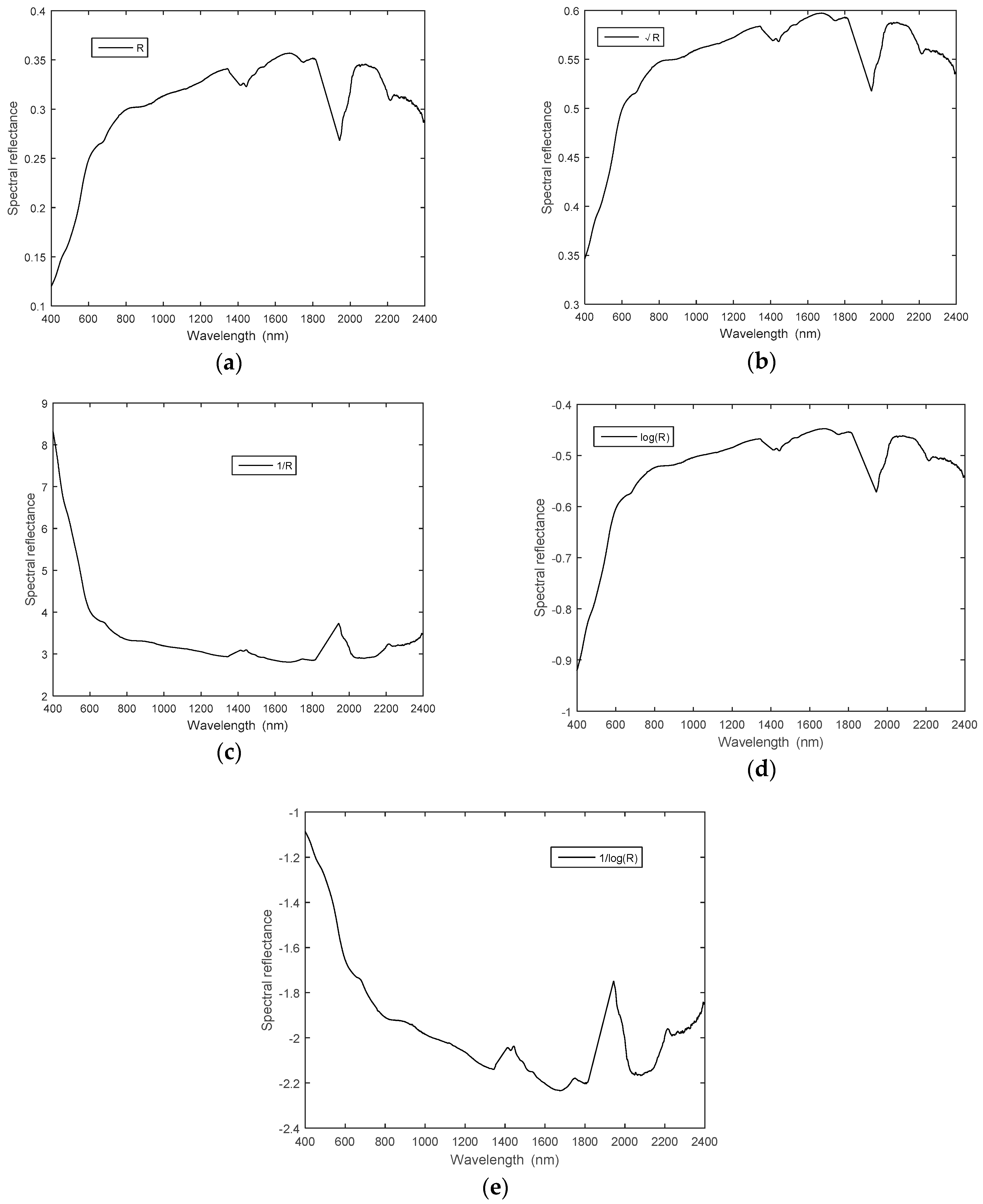
3.4. Spectral Mathematical Transformation

Before estimation model of surface parameters based on spectral reflectance is established, it is often necessary to perform nonlinear mathematical transformation for original spectral reflectance (R). The commonly used non-linear mathematical transformations include: root mean square transform ($\sqrt{\mathrm{R}}$), reciprocal transform (1/R), logarithmic transformation (lgR), and logarithm reciprocal transformation (1/lgR). The main purpose is that linear relationship between spectral reflectance and surface parameters is transformed into a nonlinear relationship, a relatively simple linear regression analysis is performed to obtain approximately nonlinear results, and various forms of estimation models are established to improve the recognition accuracy. In addition, non-linear transformation can enhance spectral difference to some extent; it is convenient to distinguish the influence on spectrum caused by the difference of surface parameters. Spectral reflectance R and its four kinds of spectral transformation curves are shown in Figure 2.

4. Simulation Results

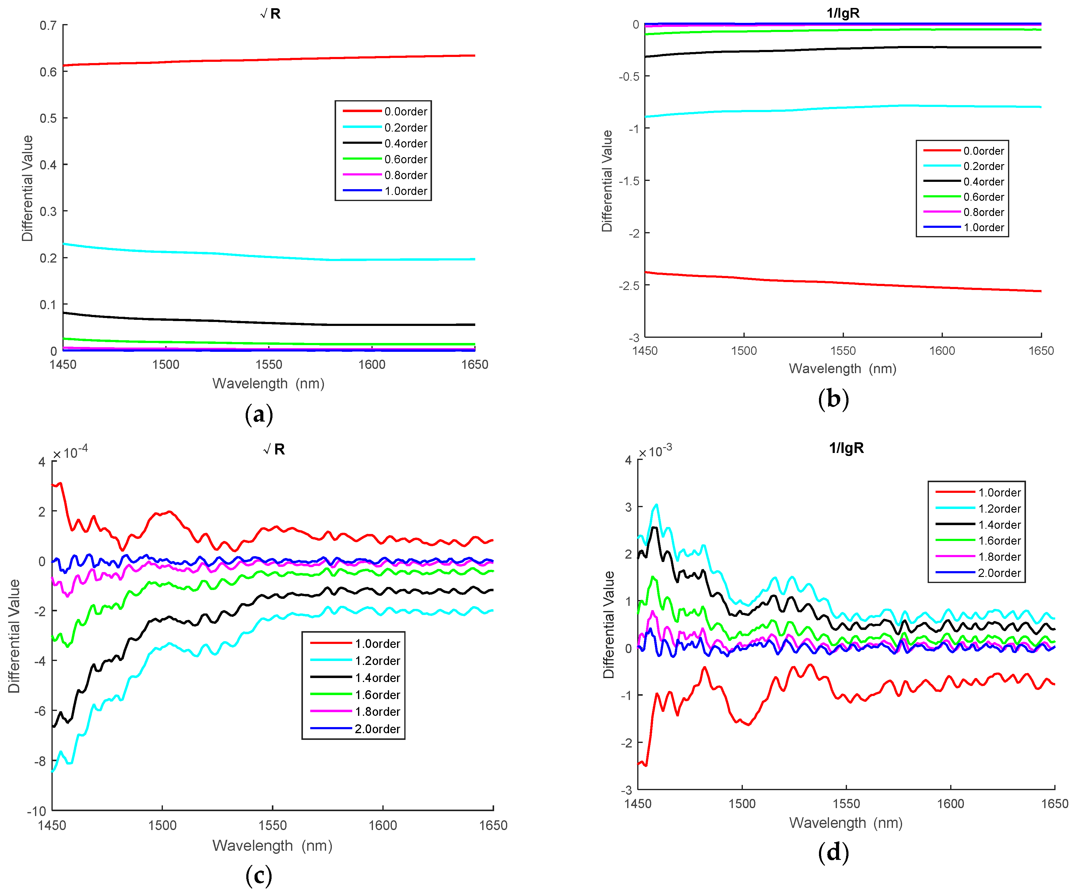
4.1. Differential Calculation of Root Mean Square and Logarithm Reciprocal

To study the effects on spectral data by fractional differentials in detail, starting differential order is 0, termination differential order is 2, and order interval is 0.2. The results of differential calculation in the bands 1450 nm and 1650 nm of soil ground hyperspectral curve for root mean square transformation and logarithm reciprocal transformation are shown in Figure 3. Differential values of two spectral transformations gradually approach 0, as the order slowly ascends from 0-order to 1-order, fractional differential curve gradually approximates the first-order differential curve. When the order is gradually increased from 1-order to 2-order, fractional derivative curve slowly approaches the 2-order differential curve, which verifies the sensitivity of fractional derivative to some extent. In addition, it can be also seen in Figure 3c,d that the derivative value in the band 1450–1550 nm fluctuates greatly, while the derivative value in the band 1550–1650 nm is less fluctuating.

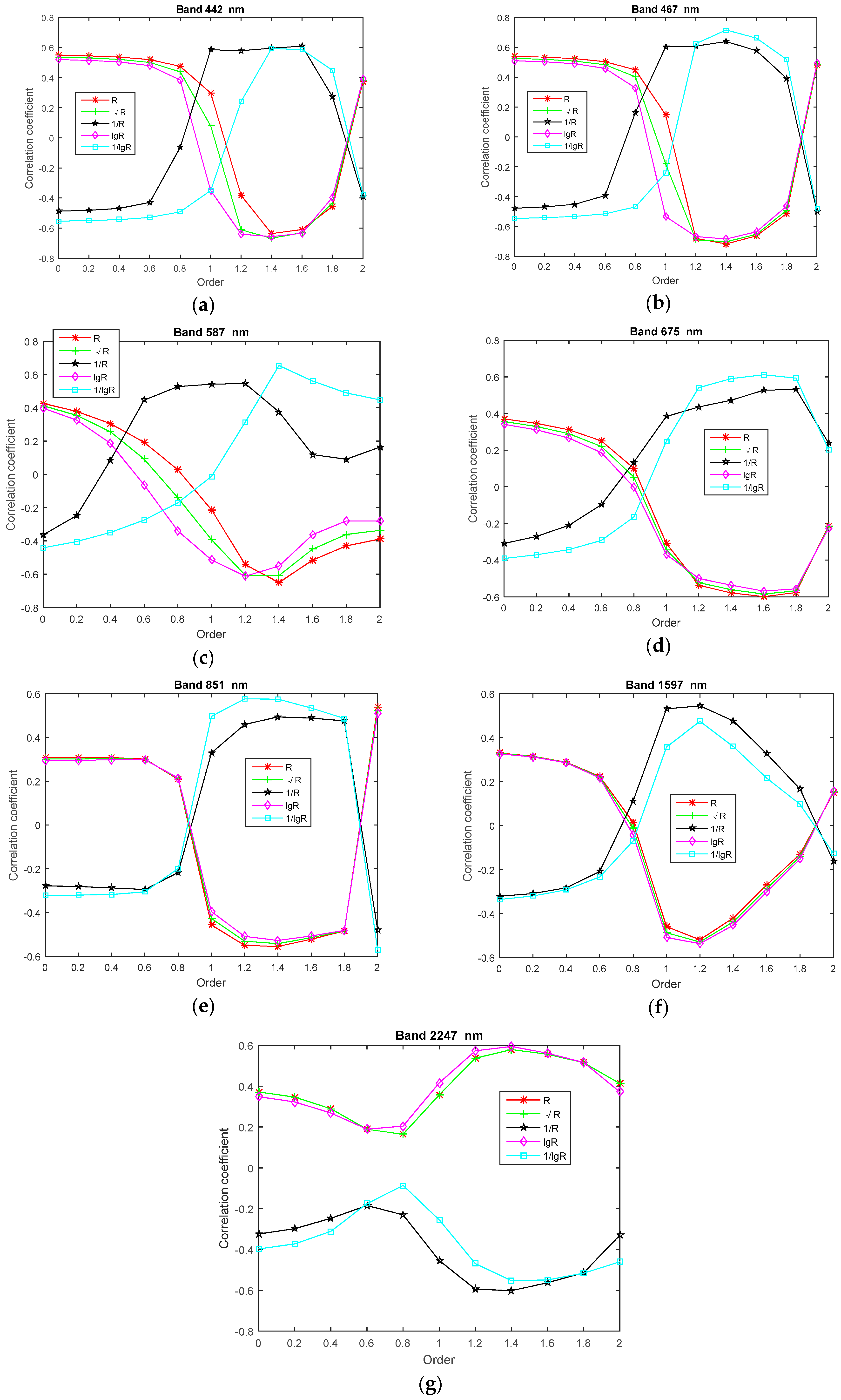
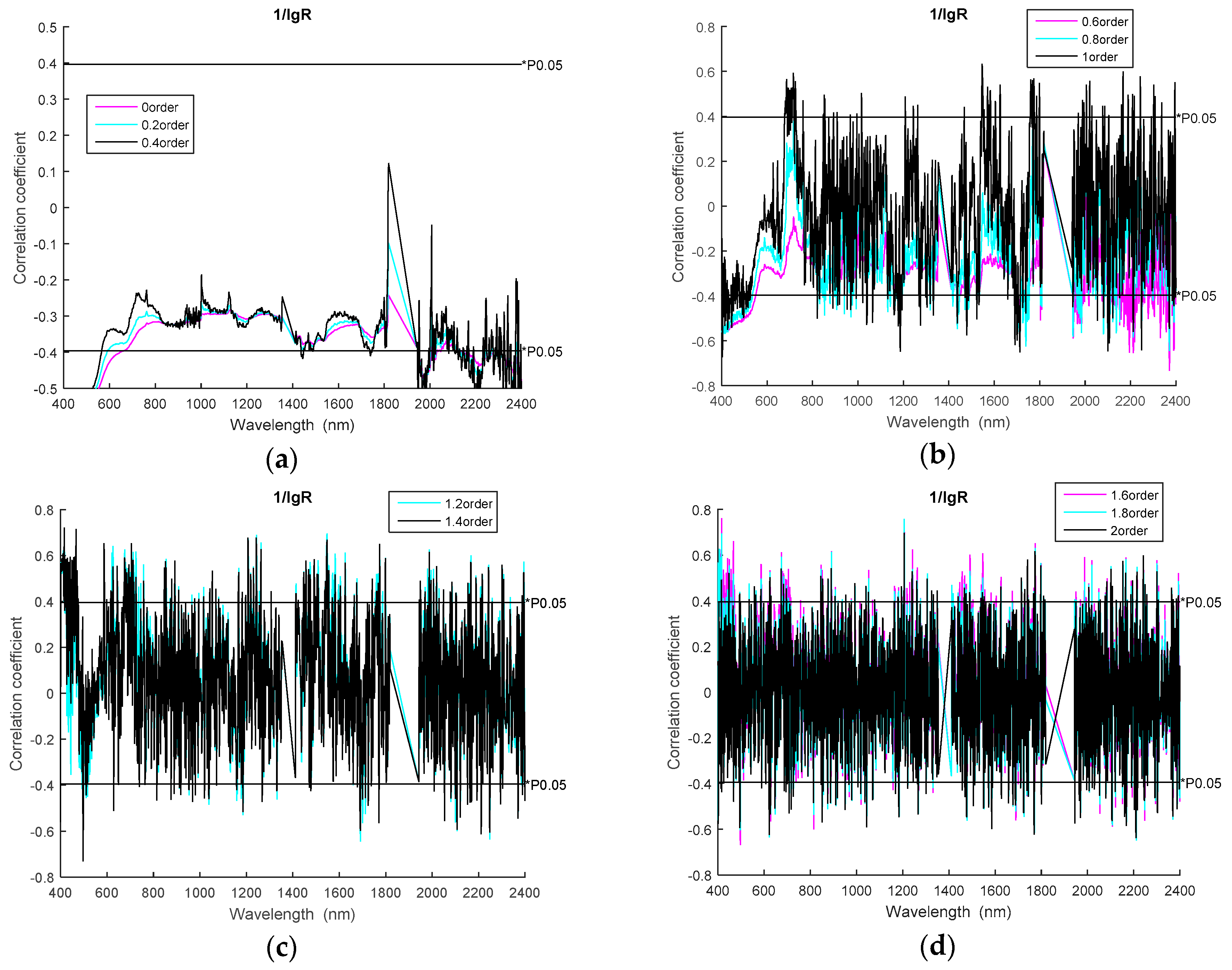
4.2. Trends of Correlation Coefficients for Root Mean Square and Logarithm Reciprocal

Correlation analysis is a key step in spectral data preprocessing. When the correlation coefficient between available potassium and spectral signal passes the significance test, the corresponding band is likely to become the sensitive band, and the band reflectance can be used as the independent variable in the model to establish a reliable predictive model of available potassium content. In this paper, the significance test was carried out at 0.05 level, and the calculus was programmed in Matlab software (MathWorks, Natick, MA, USA) to calculate the correlation between the spectral reflectance and the available potassium content after root mean square and logarithmic inverse transformation, and the differential results between 0-order and 2-order were calculated (at intervals of 0.2). The simulation results are shown in Figure 4 and Figure 5. When differential order gradually increases from zero-order to first-order, the curve of correlation coefficient shows a certain gradual change trend. When the order is increased from 1-order to 2-order, correlation coefficient curve fluctuates greatly, and the gradual change trend is not obvious.

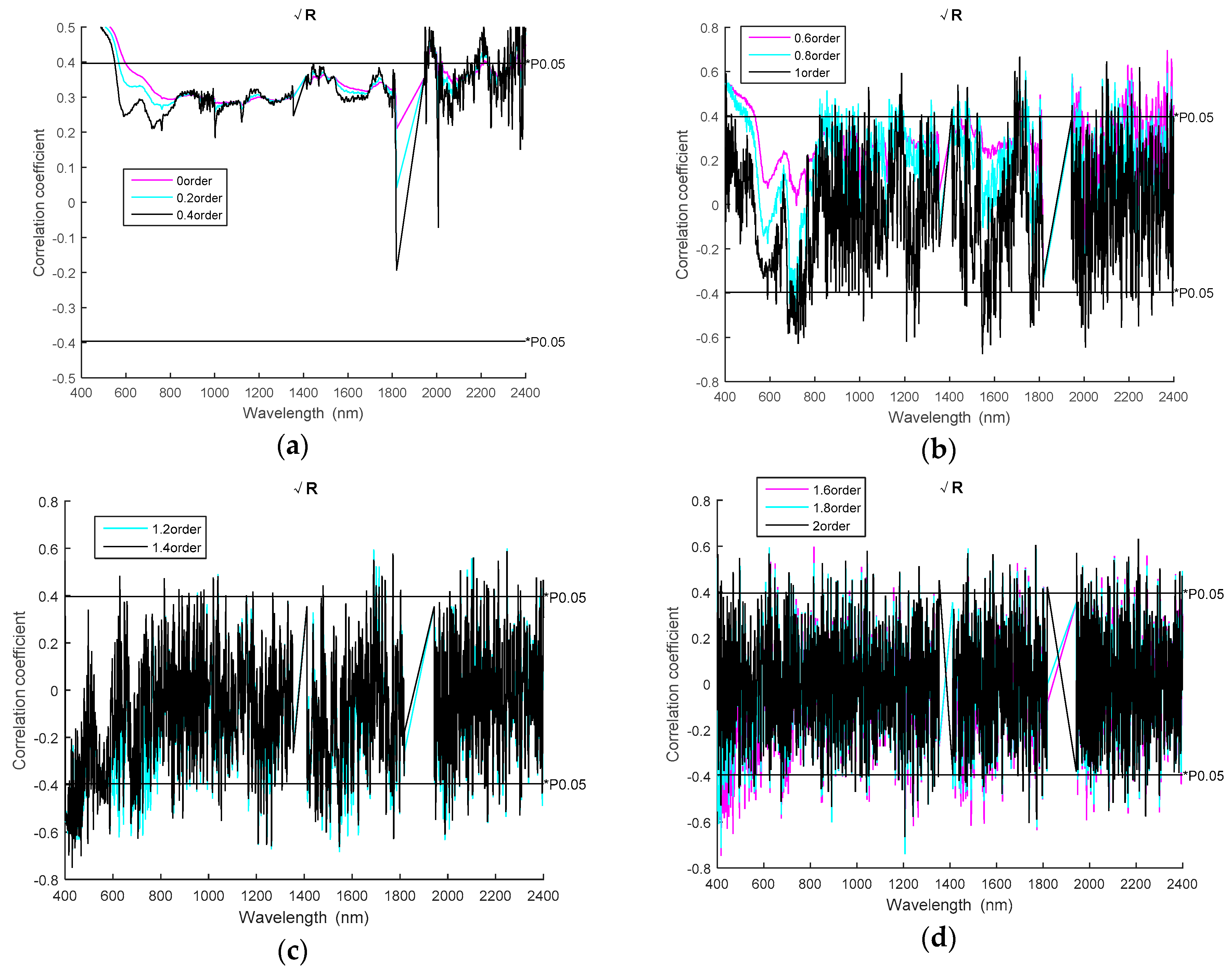
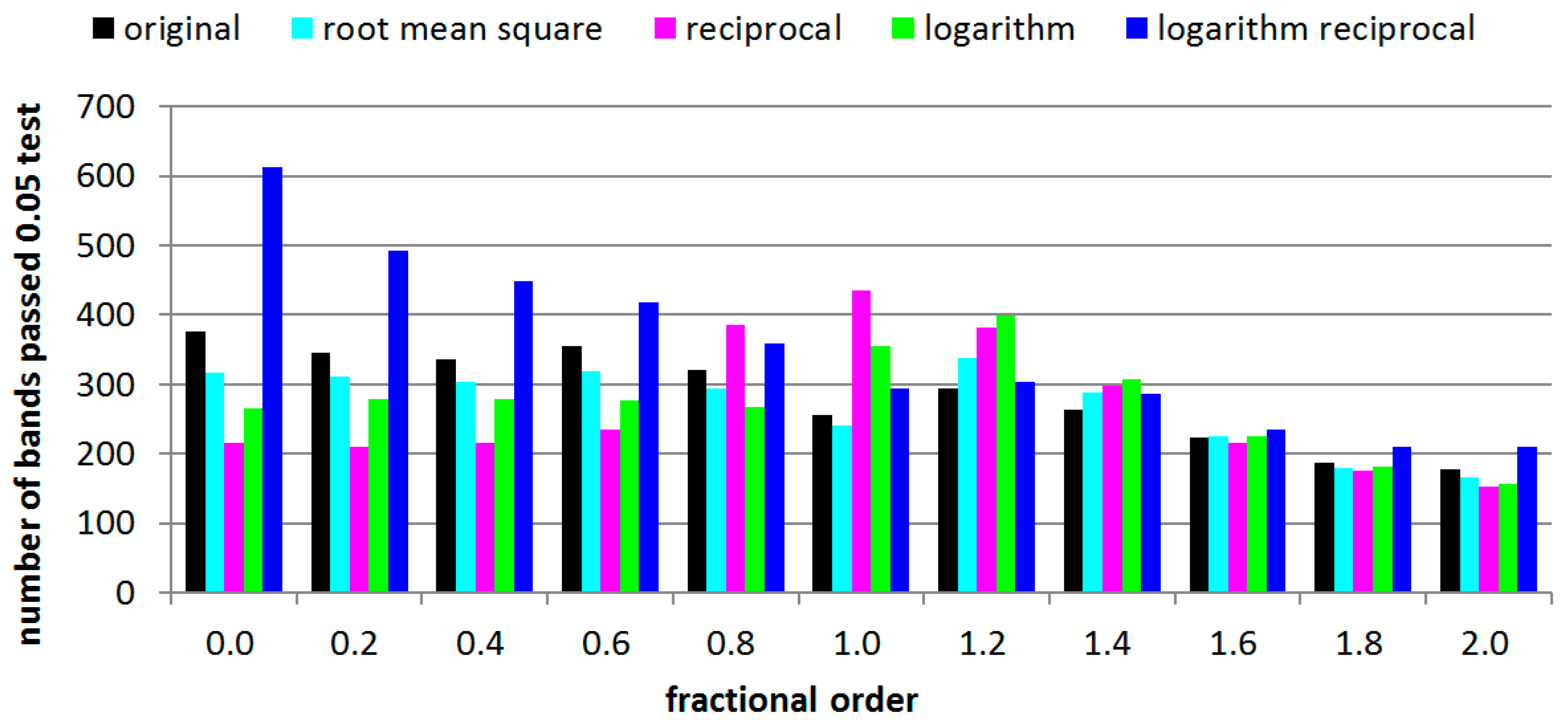
4.3. Number of Bands that Passed 0.05 Significance Level Test

The number of spectral bands that passed the 0.05 significance level of the correlation coefficient between spectrum and available potassium is shown in Figure 6. There are hundreds of spectral bands passed the 0.05 significance level for these five spectral transformations. Compared with more than 2000 full-band spectra in the range of 350–2500 nm, Figure 6 shows that the preprocessing operation of fractional calculus can reduce the dimensionality of soil hyperspectral data. Overall, the trend of the number for logarithm reciprocal, original spectrum and root mean square is gradually decreasing, and the trend increases first and then decreases for reciprocal and logarithm.

4.4. Absolute Maximum Band of Correlation Coefficient under Five Spectral Transformations

Maximum absolute values of correlation coefficients under five different spectral transformations in the 0-order to 2-order range and the corresponding band information are shown in

Table 1. Bands with the largest absolute values of correlation coefficients under five spectral transformation.

Order	R		$\sqrt{\mathbf{R}}$		1/R		lgR		1/lgR
	Largest Absolute	Band	Largest Absolute	Band	Largest Absolute	Band	Largest Absolute	Band	Largest Absolute	Band
0	0.560973	405	0.547695	405	0.499854	400	0.532827	405	0.562356	405
0.2	0.570438	2391	0.559709	2391	0.521992	2392	0.547824	2392	0.586224	2391
0.4	0.700301	2390	0.690903	2391	0.655011	2391	0.680045	2391	0.719717	2390
0.6	0.712129	2371	0.697076	2371	0.645772	2390	0.680265	2371	0.734104	2371
0.8	0.632373	2100	0.62877	2100	0.663153	2006	0.623198	2100	0.645372	2371
1	0.668786	1547	0.675601	1547	0.674436	2006	0.674577	1547	0.67265	404
1.2	0.707065	416	0.746563	430	0.674899	495	0.747359	495	0.705747	416
1.4	0.722362	416	0.750124	430	0.741574	494	0.739563	430	0.730641	497
1.6	0.763605	416	0.746466	416	0.689794	1207	0.725154	416	0.762187	416
1.8	0.74986	1207	0.739655	1207	0.701802	416	0.726421	1207	0.75847	1207
2	0.678462	1206	0.664644	1206	0.621093	1740	0.648568	1206	0.69792	1206

. The maximum absolute values of correlation coefficients appear in fractional order: when R and 1/lgR are in the 1.6 order, the corresponding band is 416 nm, and the largest absolute of R and 1/lgR are 0.763605 and 0.76218, respectively; when 1/R and $\sqrt{\mathrm{R}}$ are in the 1.4-order, the corresponding bands are 494 and 430 nm, and the largest absolute of 1/R and $\sqrt{\mathrm{R}}$ are 0.741574 and 0.750124, respectively; and when lgR is in the 1.2-order, the corresponding band is 495 nm, and the largest absolute is 0.747359. For first-order differential transformation,$\sqrt{\mathrm{R}}$, 1/R, lgR, and 1/lgR increase the correlation between spectral reflectance of R and available potassium content to some extent. For 0-order and 2-order differential transformation, 1/lgR improves the correlation, while the others reduce the correlation. In addition, the absolute values of correlation coefficients of 1.2-, 1.4-, 1.6-, and 1.8-order for R,$\sqrt{\mathrm{R}}$, lgR, and 1/lgR are all greater than 0.7.

4.5. Fractional Derivative Impact on Correlation Coefficient of Landsat 8 Image Bands

To further explain the influence of correlation on partial bands by fractional derivative, seven bands corresponding to Landsat 8 image [28,29] were selected to study the variation trend of the correlation coefficient under different fractional order. The band ranges of Landsat 8 image are shown in

Table 2. Spectral ranges of Landsat 8 image bands.

Band name	Band range (nm)
Band 1 Coastal	433–453
Band 2 Blue	450–515
Band 3 Green	525–600
Band 4 Red	630–680
Band 5 NIR	845–885
Band 6 SWIR1	1560–1660
Band 7 SWIR2	2100–2300

. The seven wavelength bands selected from Landsat 8 are 442 nm in Band 1, 467 nm in Band 2, 587 nm in Band 3, 675 nm in Band 4, 851 nm in Band 5, 1597 nm in Band 6, and 2247 nm in Band 7. The trend of correlation coefficient for the seven selected wavelength bands is shown in Figure 7.

It can be seen in Figure 7 that the correlation coefficient change of R and 1/lgR is opposite to the other three transformations. In Band 7, the correlation coefficients of 1/R and 1/lgR are negative at 0-order to 2-order, and the remaining transformations are positive. In the range of Band 1, Band 2, Band 4, Band 5 and Band 6, the correlation coefficients of 1/R and 1/lgR are negative at 0-order to 0.6-order, and the remaining transformations are positive at 0.0–0.6 order. The correlation coefficients of 1/R and 1/lgR are positive at 1.2-order to 1.8-order, and the remaining transformations are negative at 1.2-order to 1.8-order. In addition, the maximum absolute correlation coefficient of five spectral transformations is in Band 2, which is 0.715766 of 467 nm.

5. Discussion

The integer-order derivative method is widely used in soil spectral signal pretreatment, but its description of the physical model is only an approximation [30,31]. This traditional preprocessing method based on integer-order derivative has obvious shortcomings. One of the main reasons is the defect of integer-order derivative in the numerical calculation process, that is, the integer-order derivative is only related to the information of the points in the differential window. Another main reason is that the fractional derivative has the advantage of “memory” and “non-locality”, that is, the fractional order is not only related to the value of the point, but also related to the value of all points before this point. It has been proved that the fractional-order system is more in line with the laws of nature and engineering physics, which can better reflect the performance of the dynamic system, and has a unique historical memory function. Therefore, the fractional derivative model is more accurate than the integer-order derivative model.

In addition to the pretreatment of hyperspectral signals for saline soil between spectral reflectance and salt content, fractional derivatives can also be used to pretreat other types of soil hyperspectral signals between spectral reflectance and nutrient content. For example, Xia et al. [32] used fractional derivative to preprocess the spectrum collected in Ebinur Lake of Xinjiang, China, and the correlation coefficient between electricity conductivity and soil reflectance spectra was analyzed. Results show that fractional derivative details the varying trends of soil reflectance spectra among 0-order to 2-order. Fractional derivative also raises the correlation coefficient between electricity conductivity and soil reflectance spectra for some bands. Hong et al. [33] applied the fractional derivative to analyze the relationship of soil organic matter content and visible and near-infrared spectroscopy. The results show that the highest validation model appears in the 1.5-order derivative combined genetic algorithm. Wang et al. [34] collected 168 sample of soil taken from the coalmine in Eastern Junggar Basin, China. They used fractional derivative to preprocess the hyperspectral data of coalmine soil and PLSR to estimate the soil chromium content. The results show that 1.8-order derivative is the best predictive model, and the ratio of performance to deviation (PRD) is 2.14. Wang et al. [35] used the soil of the Ebinur Lake Wetland National Nature Reserve in Xinjiang as the research object, and used the fractional differential and grey correlation analysis-BP neural network to quantitatively estimate the soil organic matter content. The results show that the 1.2-order model has the highest accuracy and the PRD value is 2.26.

In addition, fractional derivatives are also used to preprocess hyperspectral signals from rubber trees, diesel, tobacco, wheat, corn, and so on. For example, Chen et al. [36] adopted fractional derivative to analyze the near-infrared spectroscopy of nitrogen concentration for natural rubber. The results show that the 0.6-order has the optimal prediction result. Tong et al. [37] adopted SG derivation to analyze the near-infrared spectroscopy of diesel dataset and tobacco dataset. The results show that this method can improve the spectral resolution, and SG derivation combined with competitive adaptive reweighted sampling is the optimal model.

6. Conclusions

Fractional derivative in the field of hyperspectral studies are rarely reported, especially for field-measured ground hyperspectral data. We collected soil samples and hyperspectral data in May 2017. Grünwald–Letnikov fractional derivative was used to analyze the correlation coefficient between the available potassium content and the soil ground hyperspectral data and Landsat 8 multispectral satellite data. Simulation results display that the small difference between spectrum data was clearly described by fractional derivative. The maximum absolute correlation coefficient appeared in the fractional order for the ground hyperspectral data and Landsat 8 multispectral satellite data. Therefore, fractional derivative enriches the pre-processing method of spectral data, provides potential spectrum information, increases the correlation coefficient between spectral reflectance and available potassium content, and provides scientific support for local precision agriculture.

References

1. Sardans, J.; Penuelas, J. Potassium: A neglected nutrient in global change. Glob. Ecol. Biogeogr. 2015, 24, 261–275. [Google Scholar] [CrossRef]
2. Qiu, K.; Xie, Y.; Xu, D.; Pott, R. Ecosystem functions including soil organic carbon, total nitrogen and available potassium are crucial for vegetation recovery. Sci. Report. 2018, 8, 7607. [Google Scholar] [CrossRef] [PubMed]
3. Panda, R.; Patra, S.K. Assessment of Suitable Extractants for Predicting Plant-available Potassium in Indian Coastal Soils. Commun. Soil Sci. Plant Anal. 2018, 49, 1157–1167. [Google Scholar] [CrossRef]
4. Viscarra Rossel, R.A.; Walvoort, D.J.J.; McBratney, A.B.; Janik, L.J.; Skjemstad, J.O. Visible, near infrared, mid infrared or combined diffuse reflectance spectroscopy for simultaneous assessment of various soil properties. Geoderma 2006, 131, 59–75. [Google Scholar] [CrossRef]
5. Jia, S.; Yang, X.; Li, G.; Zhang, J. Quantitatively determination of available phosphorus and available potassium in soil by near infrared spectroscopy combining with recursive partial least squares. Spectro. Spectr. Anal. 2015, 35, 2516–2520. [Google Scholar]
6. Sarkar, S.; Patra, S.K. Evaluation of Chemical Extraction Methods for Determining Plant-Available Potassium in Some Soils of West Bengal, India. Commun. Soil Sci. Plant Anal. 2017, 48, 1008–1019. [Google Scholar] [CrossRef]
7. Zhang, L.; Zhang, M.; Ren, H.; Pu, P.; Kong, P.; Zhao, H. Comparative investigation on soil nitrate-nitrogen and available potassium measurement capability by using solid-state and PVC ISE. Comput. Electr. Agric. 2015, 112, 83–91. [Google Scholar] [CrossRef]
8. O’Rourke, S.M.; Stockmann, U.; Holden, N.M.; McBratney, A.B.; Minasny, B. An assessment of model averaging to improve predictive power of portable vis-NIR and XRF for the determination of agronomic soil properties. Geoderma 2016, 279, 31–44. [Google Scholar] [CrossRef]
9. Gholizadeh, A.; Saberioo, M.; Ben-Dor, E.; Boruvka, L. Monitoring of selected soil contaminants using proximal and remote sensing techniques: Background, state-ofthe-art and future perspectives. Crit. Rev. Environ. Sci. Tech. 2018, 48, 243–278. [Google Scholar] [CrossRef]
10. Lamine, S.; Petropoulos, G.P.; Brewer, P.A.; Bachari, N.E.; Srivastava, P.K.; Manevski, K.; Kalaitzidis, C.; Macklin, M.G. Heavy Metal Soil Contamination Detection Using Combined Geochemistry and Field Spectroradiometry in the United Kingdom. Sensors 2019, 19, 762. [Google Scholar] [CrossRef]
11. Liu, X.; Wang, L.; Chang, Q.; Wang, X.; Shang, Y. Prediction of total nitrogen and alkali hydrolysable nitrogen content in loess using hyperspectral data based on correlation analysis and partial least squares regression. Chin. J. Appl. Ecol. 2015, 26, 2107–2114. [Google Scholar]
12. Debaene, G.; Niedźwiecki, J.; Pecio, A.; Żurek, A. Effect of the number of calibration samples on the prediction of several soil propertiesat the farm-scale. Geoderma 2014, 214/215, 114–125. [Google Scholar] [CrossRef]
13. Mashimbye, Z.E.; Cho, M.A.; Nell, J.P.; Declercq, W.P.D.; Niekerk, A.V.; Turner, D.P. Model-Based Integrated Methods for Quantitative Estimation of Soil Salinity from Hyperspectral Remote Sensing Data A Case Study of Selected South African Soils. Pedosphere 2012, 22, 640–649. [Google Scholar] [CrossRef]
14. Yang, H.; Kuang, B.; Mouazen, A.M. Quantitative analysis of soil nitrogen and carbon at a farm scale using visible and near infrared spectroscopy coupled with wavelength reduction. Eur. J. Soil Sci. 2011, 63, 410–420. [Google Scholar] [CrossRef]
15. Fu, Y.; Yang, G.; Wang, J.; Song, X.; Feng, H. Winter wheat biomass estimation based on spectral indices, band depth analysis and partial least squares regression using hyperspectral measurements. Comput. Electr. Agric. 2014, 100, 51–59. [Google Scholar] [CrossRef]
16. Wu, Q.; Yang, Y.; Xu, Z.; Jin, Y.; Guo, Y.; Lao, C. Applying Local Neural Network and Visible/Near-Infrared Spectroscopy to Estimating Available Nitrogen, Phosphorus and Potassium in Soil. Spectro. Spectr. Anal. 2014, 34, 2102–2105. [Google Scholar]
17. Liu, X.; Liu, J. Based on the LS-SVM Modeling Method Determination of Soil Available N and Available K by Using Near-Infrared Spectroscopy. Spectro. Spectr. Anal. 2012, 32, 3019–3023. [Google Scholar]
18. Wang, J.; Tiyip, T.; Ding, J.; Zhang, D.; Liu, W.; Wang, F.; Nigara, T. Desert soil clay content estimation using reflectance spectroscopy preprocessed by fractional derivative. PLOS ONE 2017, 12, e0184836. [Google Scholar] [CrossRef]
19. Wang, J.; Ding, J.; Aerzuna, A.; Cai, L. Quantitative estimation of soil salinity by means of different modeling methods and visible-near infrared (VIS-NIR) spectroscopy, Ebinur Lake Wetland, Northwest China. PeerJ 2018. [Google Scholar] [CrossRef]
20. Kaslik, E.; Sivasundaram, S. Non-Existence of Periodic Solutions in Fractional-Order Dynamical Systems and a Remarkable Difference Between Integer and Fractional-Order Derivatives of Periodic Functions. Nonlinear Anal. Real World Appl. 2012, 13, 1489–1497. [Google Scholar] [CrossRef]
21. Mbouna, G.S.; Woafo, P. Dynamics and Synchronization Analysis of Coupled Fractional-Order Nonlinear Electromechanical Systems. Mech. Res. Commun. 2012, 46, 20–25. [Google Scholar]
22. Wu, L.; Liu, S.; Yao, L.; Yan, S.; Liu, D. Grey System Model with the Fractional Order Accumulation. Commun. Nonlinear Sci. Numer. Simul. 2013, 18, 1775–1785. [Google Scholar] [CrossRef]
23. Galeone, L.; Garrappa, R. Explicit Methods for Fractional Differential Equations and Their Stability Properties. J. Comput. Appl. Math. 2009, 228, 548–560. [Google Scholar] [CrossRef]
24. Schmitt, J.M. Fractional Derivative Analysis of Diffuse Reflectance Spectra. Appl. Spectro. 1998, 52, 840–846. [Google Scholar] [CrossRef]
25. Zheng, K.; Zhang, X.; Tong, P.; Yao, Y.; Du, Y. Pretreating near infrared spectra with fractional order Savitzky–Golay differentiation (FOSGD). Chin. Chem. Letters 2015, 26, 293–296. [Google Scholar] [CrossRef]
26. Zhang, D.; Tiyip, T.; Ding, J.; Zhang, F.; Nurmemet, I.; Kelimu, A.; Wang, J. Quantitative Estimating Salt Content of Saline Soil Using Laboratory Hyperspectral Data Treated by Fractional Derivative. J. Spectro. 2016. [Google Scholar] [CrossRef]
27. Liu, Y.; Liu, Y.; Chen, Y.; Zhang, Y.; Shi, T.; Wang, J.; Hong, Y.; Fei, T.; Zhang, Y. The Influence of Spectral Pretreatment on the Selection of Representative Calibration Samples for Soil Organic Matter Estimation Using Vis-NIR Reflectance Spectroscopy. Remote Sens. 2019, 11, 450. [Google Scholar] [CrossRef]
28. Zhang, K.; Dong, X.; Liu, Z.; Gao, W.; Hu, Z.; Wu, G. Mapping Tidal Flats with Landsat 8 Images and Google Earth Engine: A Case Study of the China’s Eastern Coastal Zone circa 2015. Remote Sens. 2019, 11, 924. [Google Scholar] [CrossRef]
29. Lima, T.A.; Beuchle, R.; Langner, A.; Grecchi, R.; Griess, V.C.; Frédéric, A. Comparing Sentinel-2 MSI and Landsat 8 OLI Imagery for Monitoring Selective Logging in the Brazilian Amazon. Remote Sens. 2019, 11, 961. [Google Scholar] [CrossRef]
30. Nawar, S.; Buddenbaum, H.; Hill, J.; Kozak, J.; Mouazen, A.M. Estimating the soil clay content and organic matter by means of different calibration methods of VIS–NIR diffuse reflectance spectroscopy. Soil Tillage Res. 2016, 155, 510–522. [Google Scholar] [CrossRef]
31. Srivastava, R.; Sarkar, D.; Mukhopadhayay, S.S.; Sood, A.; Singh, M.; Nasre, R.A.; Dhale, S.A. Development of hyperspectral model for rapid monitoring of soil organic carbon under precision farming in the Indo-Gangetic Plains of Punjab, India. J. Indian Soc. Remote Sens. 2015, 43, 751–759. [Google Scholar] [CrossRef]
32. Xia, N.; Tiyip, T.; Kelimu, A.; Nurmemet, I.; Ding, J.; Zhang, F.; Zhang, D. Influence of Fractional Differential on Correlation Coefficient between EC1:5 and Reflectance Spectra of Saline Soil. J. Spectro. 2017. [Google Scholar] [CrossRef]
33. Hong, Y.; Chen, Y.; Yu, L.; Liu, Y.; Liu, Y.; Zhang, Y.; Liu, Y.; Cheng, H. Combining Fractional Order Derivative and Spectral Variable Selection for Organic Matter Estimation of Homogeneous Soil Samples by VIS–NIR Spectroscopy. Remote Sens. 2018, 10, 479. [Google Scholar] [CrossRef]
34. Wang, J.; Tiyip, T.; Zhang, D. Spectral Detection of Chrominum Content in Desert Soil Based on Fractional Differential. Trans. Chin. Soc. Agric. Mach. 2017, 48, 152–158. [Google Scholar]
35. Wang, X.; Zhang, F.; Kung, H.; Johnson, V.C. New methods for improving the remote sensing estimation of soil organic matter content (SOMC) in the Ebinur Lake Wetland National Nature Reserve (ELWNNR) in northwest China. Remote Sens. Environ. 2018, 218, 104–118. [Google Scholar] [CrossRef]
36. Chen, K.; Li, C.; Tang, R. Estimation of the nitrogen concentration of rubber tree using fractional calculus augmented NIR spectra. Ind. Crops Product. 2017, 108, 831–839. [Google Scholar] [CrossRef]
37. Tong, P.; Du, Y.; Zheng, K.; Wu, T.; Wang, J. Improvement of NIR model by fractional order Savitzky–Golay derivation (FOSGD) coupled with wavelength selection. Chemom. Intell. Lab. Syst. 2015, 143, 40–48. [Google Scholar] [CrossRef]
Figure 1. Location of sample point.
Mathematics 07 00488 g001
Figure 2. Spectral reflectance of soil and its four mathematical transformation forms: (a) R; (b) R ; (c) 1/R; (d) lgR; and (e) 1/lgR.
Mathematics 07 00488 g002
Figure 3. Fractional differential calculation of R and 1/lgR reflectance at 1450–1650 nm: (a) 0-order to 1-order of root mean square; (b) 0-order to 1-order of logarithm reciprocal; (c) 1-order to 2-order of root mean square; and (d) 1-order to 2-order of logarithm reciprocal.
Mathematics 07 00488 g003
Figure 4. Trends of correlation coefficient for root mean square: (a) 0-order to 0.4-order; (b) 0.6-order to 1-order; (c) 1.2-order to 1.4-order; and (d) 1.6-order to 2-order.
Mathematics 07 00488 g004
Figure 5. Trends of correlation coefficient for logarithm reciprocal: (a) 0-order to 0.4-order; (b) 0.6-order to 1-order; (c) 1.2-order to 1.4-order; and (d) 1.6-order to 2-order.
Mathematics 07 00488 g005
Figure 6. Number of bands that passed the 0.05 test.
Mathematics 07 00488 g006
Figure 7. The trend of correlation coefficient for partial bands of Landsat 8 image in each order differential: (a) 442 nm; (b) 467 nm; (c) 587 nm; (d) 675 nm ; (e) 851 nm ; (f) 1597 nm; and (g) 2247 nm.
Mathematics 07 00488 g007