Logistic Growth Described by Birth-Death and Diffusion Processes

Abstract

We consider the logistic growth model and analyze its relevant properties, such as the limits, the monotony, the concavity, the inflection point, the maximum specific growth rate, the lag time, and the threshold crossing time problem. We also perform a comparison with other growth models, such as the Gompertz, Korf, and modified Korf models. Moreover, we focus on some stochastic counterparts of the logistic model. First, we study a time-inhomogeneous linear birth-death process whose conditional mean satisfies an equation of the same form of the logistic one. We also find a sufficient and necessary condition in order to have a logistic mean even in the presence of an absorbing endpoint. Then, we obtain and analyze similar properties for a simple birth process, too. Then, we investigate useful strategies to obtain two time-homogeneous diffusion processes as the limit of discrete processes governed by stochastic difference equations that approximate the logistic one. We also discuss an interpretation of such processes as diffusion in a suitable potential. In addition, we study also a diffusion process whose conditional mean is a logistic curve. In more detail, for the considered processes we study the conditional moments, certain indices of dispersion, the first-passage-time problem, and some comparisons among the processes.

1. Introduction

Several real evolutionary phenomena can be described by mathematical models, based on differential equation such as the Malthusian equation

$$\frac{dN(t)}{dt}=rN(t),t\ge 0,$$

(1)

where $N(t)$ represents the population size at the time t and $r>0$ represents the growth rate. Due to (1), $N(t)$ is given by

$$N(t)=y{e}^{rt},t\ge 0,$$

with $N(0)=y>0$.

However, the Malthusian growth model, in some instances, turns out to be not fully appropriate, indeed, for the construction of a model for long-term growth. Hence, we must take into account other factors like the availability of nutritional resources, which can slow down or speed up population growth. In this context, one of the first generalizations of the simple exponential model is the logistic equation (see, as a reference [1]):

$$\frac{dN(t)}{dt}=rN(t)\left\{1-\frac{N(t)}{C}\right\},t\ge 0,$$

(2)

where $C>0$ is the carrying capacity that represents the maximum value of the population size because of the environmental influence. Note that if C tends to infinity, the logistic growth tends to the Malthusian one. Equation (2) can be further generalized, as

$$\frac{dN(t)}{dt}=r{\left[N(t)\right]}^{\alpha }{\left\{1-{\left[\frac{N(t)}{C}\right]}^{\beta }\right\}}^{\gamma },t\ge 0,$$

where $\alpha ,\beta$ and $\gamma$ are positive constants (see [2] as a reference).

In Equation (1), the growth rate r can be replaced by a time-dependent function. In this way, we obtain a more general model of population growth described by the differential equation

$$\frac{dN(t)}{dt}=\xi (t)N(t),t\ge 0,$$

(3)

where $\xi (t)$ is the time-dependent rate. Various instances of the function $\xi (t)$ listed in Table 1 lead to different growth models (see [3] for the Korf model, and [4] for various remarks on the considered models).

Table 1. Some choices of the time-dependent growth rate $\xi (t)$ and the corresponding growth curves. Parameters $\alpha$ and $\beta$ are positive constants. For Gompertz-like and modified Korf models, the quantity $y>0$ represents the initial size of the population ($N_G(0)=N_{MK}(0)=y$), whereas for Korf model A is a positive constant and the initial size is 0.

Model	$\mathit{\xi }(\mathit{t})$	$\mathit{N}(\mathit{t})$
Gompertz-like	${\xi }_G(t)=\alpha e^{-\beta t}$	$N_G(t)=yexp\left\{\frac{\alpha }{\beta }\left(1-e^{-\beta t}\right)\right\},t\ge 0$
Korf	${\xi }_K(t)=\alpha t^{-(\beta +1)}$	$N_K(t)=Aexp\left\{\frac{\alpha }{\beta }\left(1-t^{-\beta }\right)\right\},t>0$
modified Korf	${\xi }_{MK}(t)=\alpha {\left(1+t\right)}^{-(\beta +1)}$	$N_{MK}(t)=yexp\left\{\frac{\alpha }{\beta }\left[1-{(1+t)}^{-\beta }\right]\right\},t\ge 0$

Mathematical models to describe growth phenomena can be useful in many fields of interest such as biology, ecology, medicine or economics (see, for instance [5,6,7]). Frunzo et al. [8] performed a generalization of Gompertz law via a Caputo-like definition of fractional derivative. The paper aims to study the logistic growth both from a deterministic and stochastic point of view, also providing a comprehensive review of results useful in mathematical modeling of growth phenomena. Although the deterministic growth models are useful in several fields, a stochastic approach turns out to be more realistic, since it takes into account the environmental random fluctuations. We thus follow various strategies by modeling the logistic growth through time-inhomogeneous linear birth-death and diffusion processes and perform several comparisons.

The paper is organized as follows. In Section 2 the logistic growth model is showed and analyzed with specific attention to its main properties like the limits, the inflection point, the maximum specific growth rate, the lag time and the threshold crossing time. These characteristics are also compared to the corresponding ones of some known growth models.

A stochastic counterpart of the logistic growth deterministic model is studied in Section 3: it is a time-inhomogeneous linear birth-death process. In order to have a closer relation between the deterministic and the stochastic models, we find a necessary and sufficient condition to have a logistic mean for the birth-death process and we consider various instances of the individual death rate. Nevertheless, the behavior of the birth-death process may be very different from the logistic curve because the process can be absorbed at zero.

Hence, Section 4 is concerning a simple birth process which is more appropriate to describe growth behavior. In this section, we also give attention to the Fano factor, the coefficient of variation, and the first-passage-time problem, in addition to the transition probabilities, the mean and the variance.

Then, in Section 5 we study some diffusion processes for the logistic growth following these strategies:

(i)

the first one leads to two diffusion processes which are the limits of sequences of discrete processes that are solutions of discrete equations obtained by approximating the deterministic equation;

(ii)

the other approach leads to a diffusion process obtained as the limit of a sequence of discrete processes which approximate the solution of the deterministic equation.

We finally perform some comparisons between the diffusion processes obtained so far.

In several fields of interest, it is useful to study diffusion processes as subject to potential, so in Section 6, we investigate the potential for the time-homogeneous diffusion processes considered so far.

2. The Logistic Model

A classical model for population growth characterized by a finite carrying capacity is the logistic growth model, originally due to Verhulst who derived his Equation (2) to describe the self-limiting growth of a biological population. We start considering the logistic Equation (2), where $0<N(t)<C$, $r>0$, and $C>0$. The solution yields the logistic curve, which is represented by the following function

$$N(t)=\frac{Cy}{y+(C-y)e^{-rt}},t\ge 0,$$

(4)

The initial population size is given by $N(0)=y\in (0,C)$. The logistic curve (4) can be viewed also as a solution of the differential Equation (3), for the time-dependent growth rate having the following expression:

$$\xi (t)=\frac{r(C-y)}{y{e}^{rt}+C-y},t\ge 0.$$

(5)

Note that the function given in (5) depends on the initial size $y=N(0)$ of the population, differently from the corresponding functions of the other models (see Table 1). Due to (4), the logistic function has a horizontal asymptote ${lim}_{t\to +\infty }N(t)=C$ (the so-called carrying capacity). The other three growth curves given in Table 1, exhibit a similar limit behavior since they tend to a constant as $t\to \infty$. Under the given assumptions, the four growth curves considered so far are increasing in t. Table 2 and Figure 1 show some relevant quantities of these models. Note that ${lim}_{t\to \infty }N(t)$ depends on the initial size y in the first and third case.

Table 2. Some characteristics of the growth models.

Model	$\mathit{N}(0)$	${\mathit{N}}^{\prime }(0)$	${lim}_{\mathit{t}\to \mathit{\infty }}\mathit{N}(\mathit{t})$
Gompertz-like	y	$\alpha y$	$yexp\left\{\frac{\alpha }{\beta }\right\}$
Korf	0	0	$Aexp\left\{\frac{\alpha }{\beta }\right\}$
modified Korf	y	$\alpha y$	$yexp\left\{\frac{\alpha }{\beta }\right\}$
logistic	y	$ry(1-\frac{y}{C})$	C

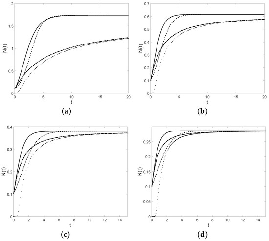
Figure 1. Gompertz-like curve $N_G$ (full), Korf curve $N_K$ (dotted), modified Korf curve $N_{MK}$ (dot-dashed), and the logistic curve N (dashed), for $y=0.1$, $A=0.1$, $\alpha =2$, $r=1$, (a) $\beta =0.7$ and $C=1.7412$, (b) $\beta =1.1$ and $C=0.6161$, (c) $\beta =1.5$ and $C=0.3794$, (d) $\beta =1.9$ and $C=0.2865$.

We note that the logistic function $N(t)$ does not always possess the characteristic S-shape: however, it is shown for some specific choices of y and C (see Figure 2).

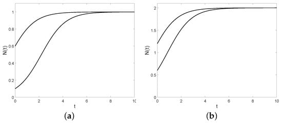
Figure 2. The logistic function $N(t)$ with $r=1$, (a): $C=1$, $y=0.1$ (bottom) and $y=0.6$ (top); (b): $C=2$, $y=0.6$ (bottom) and $y=1.2$ (top).

2.1. The Inflection Point

Let us now focus on the inflection point of the logistic model. The analysis of the inflection point is of high interest for population growth because this point represents, for sigmoidal curves, the instant when the growth rate is maximum. The second derivative of the logistic function $N(t)$ has the following expression

$$\frac{d^{2}N(t)}{d{t}^2}=\frac{r^2(C-y)\left(C-y-y{e}^{rt}\right)}{{\left(C-y+y{e}^{rt}\right)}^2}N(t),t\ge 0.$$

(6)

Hence, because of (6), if $y\ge C/2$ the logistic curve has downward concavity for $t\ge 0$, whereas, if $y<C/2$, the curve $N(t)$ is sigmoidal with inflection point

$$t_F=\frac{1}{r}log\left(\frac{C-y}{y}\right).$$

(7)

The size of the population at the inflection point is given by $N(t_F)=\frac{C}{2}$. Note that this value is independent from the choice of the initial size y (see Figure 3). In Table 3, the inflection points ($t_G,t_K,t_{MK},t_F$) and the corresponding population sizes ($N_G(t_G),N_K(t_K),N_{MK}(t_{MK}),N(t_F)$) are shown regarding the four models $N_G$, $N_K$, $N_{MK}$, and N, respectively.

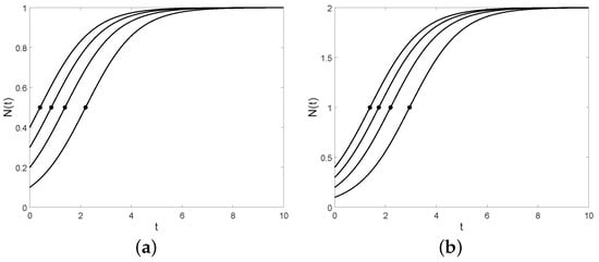
Figure 3. The logistic curve and the inflection point (asterisk point) for (a) $C=1$, (b) $C=2$, and $y=0.1,0.2,0.3,0.4$, respectively.

Table 3. The inflection points and the population sizes at these points are shown for the four models.

Model	Inflection Point	Population at the Inflection Point
Gompertz-like	$t_G=\frac{1}{\beta }log\left(\frac{\alpha }{\beta }\right),$ for $\alpha >\beta$	$N_G(t_G)=C{e}^{-1}$
Korf	$t_K={\left(\frac{\alpha }{\beta +1}\right)}^{1/\beta }$	$N_K(t_K)=C{e}^{-1-1/\beta }$
modified Korf	$t_{MK}={\left(\frac{\alpha }{\beta +1}\right)}^{1/\beta }-1,$ for $\alpha >\beta +1$	$N_{MK}(t_{MK})=C{e}^{-1-1/\beta }$
logistic	$t_F=\frac{1}{r}log\left(\frac{C-y}{y}\right),$ for $y<C/2$	$N(t_F)=C/2$

Note that

$$N_K(t_K)=N_{MK}(t_{MK})<N_G(t_G)<N(t_F),$$

consequently, even if the four curves are ordered as shown in Figure 1, the last inequality shows that the size of the population at the inflection point related to the logistic model has the greatest value among the four.

2.2. The Maximum Specific Growth Rate and the Lag Time

It may be interesting to study the growth curve in proximity of the inflection point, by approximating it with a straight line which is tangent to the curve at this point. Let us start with the definition of the maximum specific growth rate for a generic growth curve $\widehat{N}(t)$. The maximum specific growth rate $\widehat{\mu }$ is the slope of the line tangent to the curve at the inflection point $\widehat{t}$, i.e.,

$${\left.\widehat{\mu }=\frac{d\widehat{N}(t)}{dt}\right|}_{t=\widehat{t}}.$$

Moreover, the lag time $\widehat{\lambda }$ denotes the intercept with the t-axis of this tangent line. For the logistic model (4), if $y<C/2$, thanks to (7), the maximum specific growth rate is given by

$$\mu =\frac{yC(C-y)r{e}^{-r{t}_F}}{{\left(y+(C-y)e^{-r{t}_F}\right)}^2}=\frac{Cr}{4}.$$

(8)

We have obtained a value that is independent from the choice of the initial size y. Recalling the expressions of $t_F$ and $N(t_F)$ given in Table 3, the line tangent to the logistic curve at its inflection point is represented by

$$n=\mu t+\frac{C}{2}-\frac{C}{4}log\left(\frac{C-y}{y}\right),$$

with $\mu$ expressed in (8). Consequently, the lag time of the logistic model has this form:

$$\lambda =\frac{1}{r}log\left(\frac{C-y}{y}\right)-\frac{2}{r}.$$

We can notice that the lag time is positive if, and only if, $\frac{C-y}{y}>e^2$, that is if, and only if, $0<y<\frac{C}{1+e^2}$ (see Figure 4).

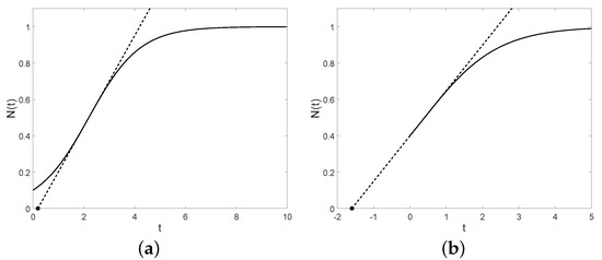
Figure 4. The tangent lines (dashed) and the lag times (asterisk points) with $C=1$, $r=1$, and (a) $y=0.1$, (b) $y=0.4$.

Table 4 shows the values of the maximum specific growth rate and the lag time for the four models of interest.

Table 4. The maximum specific growth rate, the intercept of the tangent line and the lag time for the considered growth models.

$\widehat{\mathit{N}}(\mathit{t})$	$\widehat{\mathit{\mu }}$	Intercept of Tangent Line	$\widehat{\mathit{\lambda }}$
Gompertz-like	$y\beta e^{\alpha /\beta -1}$	$y{e}^{\alpha /\beta -1}\left(1-log\frac{\alpha }{\beta }\right)$	$\frac{1}{\beta }log\frac{\alpha }{\beta }-\frac{1}{\beta }$
Korf	$A\frac{{(\beta +1)}^{1/\beta +1}}{{\alpha }^{1/\beta }}{e}^{\frac{\alpha -1}{\beta }-1}$	$-A\beta e^{\frac{\alpha -1}{\beta }-1}$	$\beta \frac{{\alpha }^{1/\beta }}{{(\beta +1)}^{1/\beta +1}}$
modified Korf	$y\frac{{(\beta +1)}^{1/\beta +1}}{{\alpha }^{1/\beta }}{e}^{\frac{\alpha -1}{\beta }-1}$	$y{e}^{\frac{\alpha -1}{\beta }-1}\left[\frac{{\left(\beta +1\right)}^{1/\beta +1}}{{\alpha }^{1/\beta }}-\beta \right]$	$\beta \frac{{\alpha }^{1/\beta }}{{(\beta +1)}^{1/\beta +1}}-1$
logistic	$\frac{Cr}{4}$	$\frac{C}{2}-\frac{C}{4}log\frac{C-y}{y}$	$\frac{1}{r}log\frac{C-y}{y}-\frac{2}{r}$

The tangent lines and the lag times of the four models are plotted in Figure 5. Considering an already mature ideal population, we can model its growth by a straight line whose slope is the maximum specific growth rate. In this context, the lag time represents the initial value of the ideal population, so that its size at time $t_F$ is $N(t_F)$.

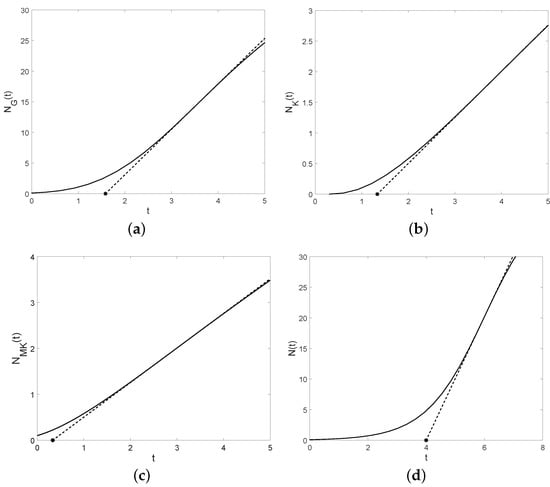
Figure 5. The tangent lines (dashed lines) and the lag times (asterisk points) with $y=0.1$, $A=0.1$, $\alpha =3$, $\beta =0.5$, $C=40.34$, and $r=1$ for (a) Gompertz model, (b) Korf model, (c) modified Korf model, (d) logistic model.

2.3. Threshold Crossing

Frequently, studies about population growth focus on the time that the value of the population size spends below (or above) a specific threshold that we denote by S. For a generic growth model $\widehat{N}(t)$, we intend to analyze the time instant $\widehat{\theta }$ when $\widehat{N}(t)$ crosses S, with $S>\widehat{N}(0)$. If we consider bounded populations, the threshold S represents a percentage p of the carrying capacity C:

$$S=pC,$$

with $\widehat{N}(0)<S<C$. Since, for the logistic model, y represents the initial size of the population $N(t)$ and C denotes the carrying capacity, that is the maximum value that the population size can reach, it is clear that the following condition must be fulfilled

$$\frac{y}{C}<p<1.$$

Denoting by $\theta$ the time instant in which the population size $N(t)$ crosses the threshold S, since

$$N(\theta )=\frac{Cy}{y+(C-y)e^{-r\theta }}=S=pC,$$

we have

$$p=\frac{y}{y+(C-y)e^{-r\theta }},$$

and so

$$\theta =-\frac{1}{r}log\left(\frac{y}{C-y}\right)-\frac{1}{r}log\left(\frac{1-p}{p}\right),$$

with $\frac{y}{C}<p<1$. After simple calculations, it is easy to obtain

$$\theta =t_F-\frac{1}{r}log\left(\frac{1-p}{p}\right),$$

and so we can examine if, and when, the time instant $\theta$ precedes the inflection point $t_F$. Clearly, it depends on p; in particular we have that

• when $0<p<1/2$, then $\theta <t_F$,
• when $p=1/2$, then $\theta =t_F$,
• when $1/2<p<1$, then $\theta >t_F$.

Similarly, we can determine the value of $\widehat{\theta }$ for the other three models, see Table 5 for interesting comparisons. With the purpose of comparing the threshold crossing of the four growth models, see Figure 6.

Table 5. The threshold crossing times for the considered growth models.

$\widehat{\mathit{N}}(\mathit{t})$	$\widehat{\mathit{\theta }}$
Gompertz-like	${\theta }_G=-\frac{1}{\beta }log\left(\frac{\beta }{\alpha }log\left(\frac{1}{p}\right)\right),$ with $e^{-\alpha /\beta }<p<1$
Korf	${\theta }_K={\left(\frac{\beta }{\alpha }log\left(\frac{1}{p}\right)\right)}^{-\frac{1}{\beta }},$ with $0<p<1$
Modified Korf	${\theta }_{MK}={\left(\frac{\beta }{\alpha }log\left(\frac{1}{p}\right)\right)}^{-\frac{1}{\beta }}-1,$ with $e^{-\alpha /\beta }<p<1$
Logistic	$\theta =-\frac{1}{r}log\left(\frac{y}{C-y}\right)-\frac{1}{r}log\left(\frac{1-p}{p}\right),$ with $\frac{y}{C}<p<1$

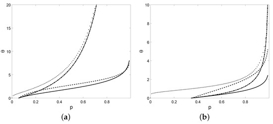
Figure 6. The threshold crossing times ${\theta }_G$ (solid), ${\theta }_K$ (dotted), ${\theta }_{MK}$ (dot-dashed), and $\theta$ (dashed) with $\alpha =2$, $y=0.1$, $A=0.1$, $r=1$, (a) $\beta =0.7$ and $C=1.7412$, (b) $\beta =1.9$ and $C=0.2865$.

3. Analysis of a Special Time-Inhomogeneous Linear Birth-Death Process

As is generally known, in various fields many growth phenomena are described by deterministic models thanks to their tractability. Nevertheless, a stochastic approach may be interesting and useful, especially because random processes take into account ubiquitous environmental fluctuations, which are due to unknown or not always quantifiable causes. Among the families of continuous-time stochastic processes typically adopted to describe population dynamics a special role is played by birth-death processes. Indeed, despite their apparently simple structure, birth-death processes are suitable to model even complex behaviors, for instance described by bimodal transition probabilities (see [9]). We recall also the recent contribution by Crawford and Suchard [10], where an efficient algorithm for computing their transition probabilities is proposed, with relevant applications in ecology, evolution, and genetics.

With the intent to introduce a stochastic counterpart of the logistic model, we now focus on an evolutionary model based on a birth-death process. Since the population size described by the logistic curve $N(t)$ can reach great values when the carrying capacity C is large, we consider a stochastic process with an infinite state-space. Specifically, we suppose that the population size can be described by an inhomogeneous linear birth-death process $\left\{X(t):t\ge 0\right\}$, with state space ${\mathbb{N}}_0:=\mathbb{N}\cup \left\{0\right\}=\{0,1,2,\dots \}$, where the state 0 is an absorbing endpoint. Clearly, the presence of an absorbing endpoint at 0 reflects realistic situations where the extinction of the population may occur. As well known, the transition rates are defined by

$$\begin{array}{cc}\hfill {\lambda }_n(t)& =\underset{h\to 0^{+}}{lim}\frac{1}{h}P\left[X(t+h)=n+1|X(t)=n\right],n\in {\mathbb{N}}_0,\hfill \\ \hfill {\mu }_n(t)& =\underset{h\to 0^{+}}{lim}\frac{1}{h}P\left[X(t+h)=n-1|X(t)=n\right],n\in \mathbb{N}.\hfill \end{array}$$

(9)

For the birth-death process under investigation, we have

$${\lambda }_n(t)=n\lambda (t),{\mu }_n(t)=n\mu (t),$$

(10)

where $\lambda (t)$ and $\mu (t)$ are positive functions, integrable on $(0,t)$ for any $t>0$. Note that the transition rates (10) are linear in n, so the probability that a single birth (or death) occurs during an infinitesimal time-interval, is proportional to the previous size n of the population and according to the time-dependent rate $\lambda (t)$ (or $\mu (t)$). We remind that the function $\lambda (t)$ (or $\mu (t)$) represents the individual birth rate (or death rate) at time t. Moreover, the model described by the transition rates given in (10) is a time-inhomogeneous version of the classical linear birth-death process (see [11]). Assume that, for $x\in {\mathbb{N}}_0$ and $y\in \mathbb{N}$, the transition probability

$$P_{yx}(t)=P\left[X(t)=x|X(0)=y\right],t\ge 0$$

(11)

denotes the probability that the number $X(t)$ of individuals of the population reaches the level x at time t, conditional on the initial size y. For the sake of non-triviality, the state $y=0$ can be excluded because it represents an absorbing endpoint for the birth-death process $X(t)$. Therefore, we will assume, from now on, that $X(0)=y\in \mathbb{N}$, in agreement with the fact that the initial value of the logistic function is positive. In order to determine the transition probability $P_{yx}(t)$, we consider the probability generating function of $X(t)$, given by

$$G(z,t)=\sum _{x=0}^{\infty }{P}_{yx}(t)z^x,0<z<1,t\ge 0,$$

with $G(z,0)=z^y$. The probability generating function has the following form, as shown in Tan [12]

$$G(z,t)={\left\{1-(z-1){\left[(z-1)\varphi (t)-\psi (t)\right]}^{-1}\right\}}^y,0<z<1,t\ge 0,$$

where

$$\psi (t)=exp\left\{-{\int }_0^t\left[\lambda (\tau )-\mu (\tau )\right]d\tau \right\},\varphi (t)={\int }_0^t\lambda (\tau )\psi (\tau )d\tau ,t\ge 0.$$

(12)

For notation convenience, we denote the mean and the variance of $X(t)$, conditional on the initial size $X(0)=y$, with $E_y(t)$ and $Va{r}_y(t)$, respectively:

$$E_y(t)=\mathbb{E}\left[X(t)|X(0)=y\right],Va{r}_y(t)=Var\left[X(t)|X(0)=y\right],t\ge 0.$$

(13)

Recalling the transition rates in (10), the conditional mean $E_y(t)$ verifies the following differential equation

$$\frac{d{E}_y(t)}{dt}=\xi (t)E_y(t),t\ge 0,$$

(14)

where $\xi (t)$ is the net growth rate per capita and is defined as follows

$$\xi (t)=\lambda (t)-\mu (t),t\ge 0.$$

(15)

Therefore, the analogies between the logistic model and the conditional mean of the birth-death process are now clear: the differential Equations (14) and (3) have the same form. So, when the conditions (15) and (5) hold, the logistic curve $N(t)$ and the mean of the birth-death process $X(t)$ are governed by the same differential equation. The transition probabilities, the conditional mean and the conditional variance of the process can be expressed in a simpler form, as shown in [4]. In particular, the transition probabilities of the process $X(t)$ with rates (10), are given by

$$P_{y0}(t)={\left(1-\frac{1}{\psi +\varphi }\right)}^y,$$

(16)

and

$$P_{yx}(t)={\left(\frac{\varphi }{\psi +\varphi }\right)}^x\sum _{i=0}^m\left(\genfrac{}{}{0pt}{}{y}{i}\right)\left(\genfrac{}{}{0pt}{}{y+x-i-1}{y-1}\right){\left({\varphi }^{-1}-1\right)}^i{\left(1-\frac{1}{\psi +\varphi }\right)}^{y-i},$$

(17)

with $x\in \mathbb{N}$, $m=min\{y,x\}$, $\psi =\psi (t)$, and $\varphi =\varphi (t)$. Moreover, the conditional mean and the conditional variance of $X(t)$ are

$$E_y(t)=\frac{y}{\psi (t)},Va{r}_y(t)=y\frac{\psi (t)+2\varphi (t)-1}{{\psi }^2(t)},t\ge 0,$$

(18)

respectively. Note that, if $\xi (t)$ is a positive function for all $t>0$, we have that both the conditional mean $E_y(t)$ and the conditional variance $Va{r}_y(t)$ are strictly increasing (see [4], as a reference). Since the state 0 is an absorbing endpoint, $P_{y,0}(t)$ represents the probability that the population dies out prior to time t conditional by the initial size $X(0)=y$. Therefore ${lim}_{t\to +\infty }{P}_{y,0}(t)$ represents the probability of an ultimate extinction and is given by

$${\pi }_{y,0}=\underset{t\to +\infty }{lim}{P}_{y,0}(t)={\left(1-\frac{1}{\tilde{\psi }+\tilde{\varphi }}\right)}^y,y\in \mathbb{N},$$

(19)

where $\tilde{\psi }={lim}_{t\to +\infty }\psi (t)$ and $\tilde{\varphi }={lim}_{t\to +\infty }\varphi (t)$.

Recalling the definition of the functions $\psi (t)$ and $\varphi (t)$ and denoting

$$\tilde{\lambda }=\underset{t\to +\infty }{lim}\lambda (t)\mathrm{and}\tilde{\mu }=\underset{t\to +\infty }{lim}\mu (t),$$

(20)

if $\tilde{\mu }-\tilde{\lambda }=\infty$ or $\tilde{\varphi }=\infty$, then ${\pi }_{y,0}=1$, so the ultimate extinction occurs almost surely. Other features on linear birth-death processes can be found in Tavaré et al. [13] and references therein.

Analysis of a Special Case

The stochastic modeling of random evolution often requires that the mean or the median of the proposed stochastic process follows a specified growth curve. An example is provided in De Lauro et al. [14], where the authors retrieve the Gompertz equation as evolution of the median of the geometric Brownian motion. Along this line, hereafter we show necessary and sufficient conditions in order that the birth-death process $X(t)$ possesses a logistic conditional mean.

Proposition 1.

The linear birth-death process with the transition rates specified in (10) has conditional mean

$$E_y(t)=\frac{Cy}{y+(C-y)e^{-rt}},t\ge 0,$$

if, and only if,

$$\xi (t)=\lambda (t)-\mu (t)=\frac{r(C-y)}{y{e}^{rt}+C-y},t\ge 0.$$

(21)

Proof. 

The conditional mean $E_y(t)$ verifies the differential Equation (14); on the other hand, the logistic curve $N(t)$ satisfies the differential Equation (3), with $\xi (t)$ specified in (5). So, the net growth rate must be chosen as shown in (5). □

From now on, we will assume that the condition (21) holds. It implies that the birth rate $\lambda (t)$ is greater than the death rate $\mu (t)$. Moreover, the net growth rate $\xi (t)$ decreases and tends to zero like a decreasing exponential function. This assumption is useful to describe a population whose conditional mean size has a S-shape. Due to (20) and (21), the difference $\tilde{\lambda }-\tilde{\mu }$ can be calculated as follows

$$\tilde{\lambda }-\tilde{\mu }=\underset{t\to +\infty }{lim}{\int }_0^t\frac{r(C-y)}{y{e}^{r\tau }+C-y}d\tau =log\frac{C}{y}.$$

The net growth rate $\xi (t)$, in this case, is a positive function so the conditional mean $E_y(t)$ is strictly increasing and tends to the carrying capacity C. Let us now specify the expressions of the functions $\psi (t)$ and $\varphi (t)$ (defined in (12)):

$$\psi (t)=exp\left\{-{\int }_0^t\xi (\tau )d\tau \right\}=\frac{y{e}^{rt}+C-y}{C{e}^{rt}},$$

(22)

with $\xi (t)$ given by (21) and $\tilde{\psi }=y/C$,

$$\varphi (t)={\int }_0^t\lambda (\tau )\left(\frac{y{e}^{r\tau }+C-y}{C{e}^{r\tau }}\right)d\tau .$$

(23)

The variance $Va{r}_y(t)$ is also strictly increasing in t, because the function $\xi (t)$ is positive for all $t>0$.

Example 1.

Let the condition (21) be satisfied. We now consider various instances of $\mu (t)$ listed in Table 6. In the last column, there are the ultimate extinction probabilities; note that, for the first three cases, we have $\tilde{\varphi }=\infty$, so the ultimate extinction probability is 1. In other words the ultimate extinction occurs as in the cases (a), (b), and (c) of Table 6. In all cases, some instances of the transition probabilities $P_{y,x}(t)$, cf. (17), are plotted in Figure 7 for $y=1$, $x=0$, and $x=1$.

Table 6. Some choices of $\mu (t)$ and the corresponding extinction probabilities. Parameters A, B, Q, and $t_0$ are positive constants.

Case	$\mathit{\mu }(\mathit{t})$	${\mathit{\pi }}_{\mathit{y},0}$
(a)	A	1
(b)	$A+B(t-t_0){\mathbb{I}}_{t\ge t_0}$	1
(c)	$A+Bsin\left(\frac{2\pi }{Q}t\right)$	1
(d)	$\frac{AC}{y{e}^{rt}+C-y}$	$<1$

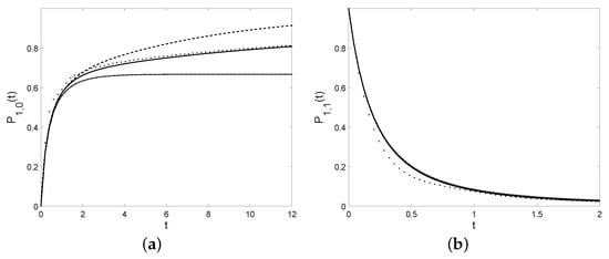
Figure 7. Probabilities (a): $P_{1,0}(t)$ and (b): $P_{1,1}(t)$, with $C=10$, $r=1$, $A=2$, $B=Q=1$ and $t_0=1$, with references to the cases specified in Table 6 (case (a): full line, case (b): dashed line, case (c): dotted line, case (d): dot-dashed line).

(a) 

If $\mu (t)=A$, with $A>0$, the populations described by the model experience constant individual death rate. The function $\varphi (t)$ is given by

$${\varphi }_a(t)=\frac{(C-y)(A+r)}{Cr}\left(1-e^{-rt}\right)+\frac{Ayt}{C},t\ge 0.$$

Thanks to (18), the variance can be calculated easily but it has a rather cumbersome form and thus is omitted for brevity.

(b) 

Let us assume $\mu (t)=A+B(t-t_0){\mathbb{I}}_{\{t\ge t_0\}}$, with $A>0$, $B>0$ and $t_0>0$. This assumption is useful to model degrading environmental or individual conditions, since it deals with an individual death rate which is constant until time $t_0$ and is linear increasing subsequently. The function $\varphi (t)$ has the following form, for $t\ge t_0$:

$${\varphi }_b(t)={\varphi }_a(t)+\frac{yB}{2C}{(t-t_0)}^2+\frac{B(C-y)}{C{r}^2}\left(\frac{r(t_0-t)-1}{e^{rt}}+\frac{1}{e^{r{t}_0}}\right).$$

Again, we omit the explicit form of the variance for brevity.

(c) 

We consider $\mu (t)=A+Bsin(\frac{2\pi }{Q}t)$, where $Q>0$ and $A>\left|B\right|>0$. This hypothesis can be used to model seasonal environmental variability, such as when the population is subject to periodically fluctuating mortality rate. In this case, we have

$$\begin{array}{cc}\hfill {\varphi }_c(t)=& {\varphi }_a(t)+\frac{By}{C}\left[\frac{Q}{2\pi }-\frac{Q}{2\pi }cos\left(\frac{2\pi t}{Q}\right)\right]\hfill \\ \hfill +& \frac{B(C-y)}{C}\left[\frac{2\pi Q}{Q^2{r}^2+4{\pi }^2}-\frac{Q\left(Qrsin\left(\frac{2\pi t}{Q}\right)+2\pi cos\left(\frac{2\pi t}{Q}\right)\right)}{(Q^2{r}^2+4{\pi }^2)e^{rt}}\right].\hfill \end{array}$$

(d) 

Let $\mu (t)=(AC){\left(y{e}^{rt}+C-y\right)}^{-1}$, with $A>0$, so the individual death rate has a behavior like a decreasing exponential function. In this case, the function $\varphi (t)$ is given by

$${\varphi }_d(t)=(1-e^{-rt})\left(\frac{C-y}{C}+\frac{A}{r}\right),t\ge 0;$$

moreover, the probability of ultimate extinction is

$${\pi }_{y,0}={\left(1-\frac{r}{r+A}\right)}^y<1,$$

and the variance has this form:

$$Va{r}_y(t)=\frac{y(C{e}^{rt})\left(r(C-y)+2AC\right)(e^{rt}-1)}{{(y{e}^{rt}+C-y)}^2}.$$

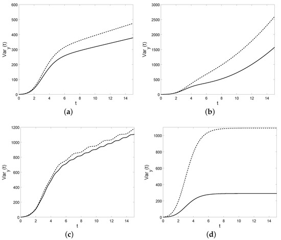
Some plots of the variance $Va{r}_y(t)$ are shown in Figure 8: note that the shape of the variance depends on $\mu (t)$. In the first three cases the variance $Va{r}_y(t)$ diverges as $t\to +\infty$, whereas in the last case it tends to a constant.

Figure 8. For $y=1$, $C=10$, the variance $Va{r}_y(t)$ is plotted for the cases of Table 6. In case (a): $A=0.6$ (solid) and $A=0.8$ (dashed). In case (b): $A=1$, $B=1$, $t_0=5$ (solid) and $t_0=1$ (dashed). In case (c): $A=2$, $B=2$, $Q=1$ (solid) and $Q=2$ (dashed). In case (d): $A=1$ (solid) and $A=5$ (dashed).

4. Analysis of a Special Time-Inhomogeneous Linear Birth Process

Even if the conditional mean of the birth-death process studied in Section 3 is identical to the logistic curve (4), the behavior of the sample paths of $X(t)$ may be significantly different from the logistic growth, because they can be absorbed at zero (see Equation (19)). Aiming to deal with dynamics closer to the logistic curve, we remove the possibility of downward jumps. In this way, we obtain a time-inhomogeneous linear birth process, which is clearly appropriate to describe pure growth phenomena. This process can be viewed as a special case of the other one considered in Section 3, which has a logistic mean. Indeed, if we take $\mu (t)=0$ in the Equation (10), the number of individuals will be modelled by an inhomogeneous linear birth process $\left\{X(t):t\ge 0\right\}$. The value $y\in \mathbb{N}$ represents the (deterministic) initial state, and the state space of $X(t)$ is the set $S=\left\{y,y+1,\cdots \right\}$. In this case, the transition rates are

$${\lambda }_n(t)=n\lambda (t),{\mu }_n(t)=0;n\in S,$$

(24)

where $\lambda (t)$ is a positive function, integrable on $(0,t)$ for any $t>0$. Again, the transition probability of $X(t)$ is defined as

$$P_{y,x}(t)=P\left[X(t)=x|X(0)=y\right],t\ge 0.$$

As shown in [15], for $y\in \mathbb{N}$ and $x\in S$, we have

$$P_{y,x}(t)=\left(\genfrac{}{}{0pt}{}{x-1}{y-1}\right)e^{-y\mathsf{\Lambda }(t)}{\left(1-e^{-\mathsf{\Lambda }(t)}\right)}^{x-y},t\ge 0,$$

(25)

where

$$\mathsf{\Lambda }(t)={\int }_0^t\lambda (\tau )d\tau ,t\ge 0.$$

The result given in Proposition 1 can be updated to our purposes in this way:

Proposition 2.

The linear birth process with rates specified in (24) has conditional mean

$$E_y(t)=\frac{Cy}{y+(C-y)e^{-rt}},t\ge 0$$

(26)

if, and only if,

$$\lambda (t)=\frac{r(C-y)}{y{e}^{rt}+C-y},t\ge 0.$$

(27)

Proof. 

The necessary and sufficient condition (27) to have conditional mean expressed by (26) holds, recalling Proposition 1 in which $\mu (t)=0$. □

When the birth rate is expressed by (27), the function $\mathsf{\Lambda }(t)$ is

$$\mathsf{\Lambda }(t)=log\left(\frac{C}{y+(C-y)e^{-rt}}\right),$$

so

$$\underset{t\to +\infty }{lim}\mathsf{\Lambda }(t)=log\frac{C}{y}.$$

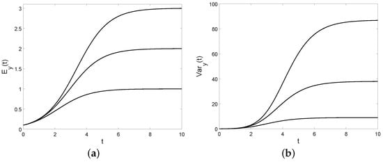
Note that by choosing the individual birth rate $\lambda (t)$ as in (27), the conditional mean of the time-inhomogeneous linear birth-process is a logistic function. According to [15], in this case both the conditional mean and the conditional variance are strictly increasing, with finite limits. The conditional mean is given by (26), with ${lim}_{t\to +\infty }{E}_y(t)=C$. The conditional variance is

$$Va{r}_y(t)=\frac{Cy}{y+(C-y)e^{-rt}}\left(\frac{C}{y+(C-y)e^{-rt}}-1\right),$$

(28)

and its limit is given by

$$\underset{t\to +\infty }{lim}Va{r}_y(t)=C\left(\frac{C}{y}-1\right).$$

In Figure 9, the conditional mean $E_y(t)$ and the conditional variance $Va{r}_y(t)$ are plotted for different choices of $C>0$; note that they are increasing in C.

Figure 9. (a): The conditional mean (26) and (b): the conditional variance (28) are plotted for $y=0.1$, $r=1$, and $C=1,2,3$ (from bottom to top). For the variance the limits are 9, 38, 87, respectively.

Let us now determine an index of dispersion called Fano factor defined as follows

$$D_y(t)=\frac{Va{r}_y(t)}{E_y(t)},t\ge 0.$$

In this case, recalling (26) and (28), we have

$$D_y(t)=\frac{C}{y+(C-y)e^{-rt}}-1,t\ge 0.$$

(29)

Note that $D_y(t)$ is increasing in t, with $D_y(0)=0$ and

$$\underset{t\to +\infty }{lim}{D}_y(t)=\frac{C}{y}-1.$$

From (29), we have that

(i)

if $y>C/2$, then the birth process $X(t)$ is underdispersed, i.e., $D_y(t)<1$ for all $t\ge 0$;

(ii)

if $y<C/2$, then the birth process $X(t)$ is underdispersed for $t<\tilde{t}$ with $\tilde{t}=\frac{1}{r}log\left(\frac{2(C-y)}{C-2y}\right)$, and $X(t)$ is overdispersed for $t>\tilde{t}$.

Due to (26) and (28), the coefficient of variation of $X(t)$ is given by

$${\sigma }_y(t)=\frac{\sqrt{Va{r}_y(t)}}{E_y(t)}={\left(\frac{C-y}{Cy}\right)}^{1/2}\sqrt{1-e^{-rt}},t\ge 0.$$

(30)

We note that ${\sigma }_y(t)$ is increasing in t and in C, whereas it is decreasing in y. The following limits hold

$$\begin{array}{ccc}\underset{t\to 0}{lim}{\sigma }_y(t)=0,\hfill & \hfill & \underset{t\to +\infty }{lim}{\sigma }_y(t)={\left(\frac{C-y}{Cy}\right)}^{1/2},\hfill \\ \underset{C\to y}{lim}{\sigma }_y(t)=0,\hfill & \hfill & \underset{C\to +\infty }{lim}{\sigma }_y(t)=y^{-1/2}\sqrt{1-e^{-rt}},\hfill \\ \underset{y\to 0^{+}}{lim}{\sigma }_y(t)=+\infty ,\hfill & \hfill & \underset{y\to C}{lim}{\sigma }_y(t)=0.\hfill \end{array}$$

Therefore, when y tends to the carrying capacity C, there is a better agreement between the logistic model (4) and the birth process with rates (24). This assumption also implies that $\lambda (t)$ tends to 0, so we expect a better correspondence between the two models when the birth rate is low. Some plots of the coefficient of variation are provided in Figure 10 for some choices of the parameters.

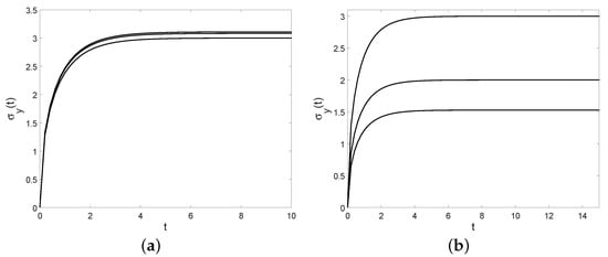
Figure 10. The coefficient of variation ${\sigma }_y(t)$ is plotted for $r=1$ and (a): $y=0.1$ and $C=1,2,3$ (from bottom to top); (b): $C=1$ and $y=0.1,0.2,0.3$ (from top to bottom).

In the remainder of this section we analyze the first-passage problem for $X(t)$, as the threshold crossing problem that we have discussed in Section 2.3. Let $y\in S$ be the initial state and $k\in \mathbb{N}$ a fixed threshold with $k>y$. The first-passage-time is defined as follows

$$T_{y,k}=inf\left\{t\ge 0:X(t)=k\right\},$$

with $X(0)=y$. Its probability density function (pdf) is denoted by $g_{y,k}(t)$. The sample paths of $X(t)$ are increasing over the state space S, since $X(t)$ is a birth process and so it is easy to see that

$$g_{y,k}(t)=(k-1)\lambda (t)P_{y,k-1}(t),$$

with $k\in \mathbb{N}$, $k>y$, $\lambda (t)$, and $P_{y,k}(t)$ defined in (27) and (25), respectively. Due to (27), $\lambda (0)=\frac{r(C-y)}{C}$ and so we can easily obtain the initial value of the first-passage-time pdf:

$$\underset{t\to 0}{lim}{g}_{y,k}(t)=\left\{\begin{array}{cc}\frac{yr(C-y)}{C},\hfill & \mathrm{if}k=y+1\hfill \\ 0\hfill & \mathrm{otherwise}.\hfill \end{array}\right.$$

(31)

Indeed, we have $P_{y,k-1}(0)=0$ for $k-1\ne y$. In Figure 11 the pdf of $T_{y,k}(t)$ is plotted for different choices of k.

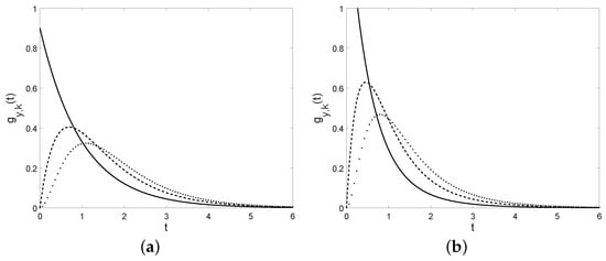
Figure 11. The probability density function of $T_{y,k}$ for $C=10$, $r=1$, (a): $k=2$ (solid), $k=3$ (dashed), $k=4$ (dotted) and $y=1$; (b): $k=3$ (solid), $k=4$ (dashed), $k=5$ (dotted) and $y=2$.

In Figure 12 the mean of the first-passage time $T_{y,k}$ is plotted as a function of C, for different choices of k and y and with $C>y$. Note that it is increasing with the respect to C in the first case, whereas in the second case it is not monotonic, but it is increasing for small values of C and decreasing for greater values of C.

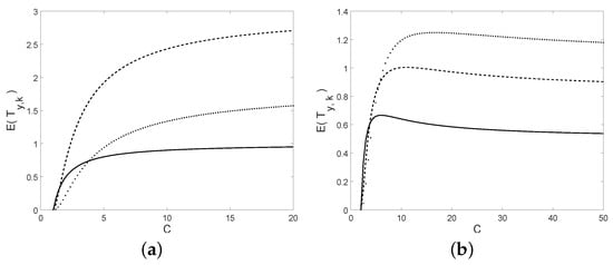
Figure 12. The mean of $T_{y,k}$ is plotted as a function of C; (a): for $y=1$ and $k=2$ (solid), $k=3$ (dotted), $k=4$ (dashed); (b): for $y=2$ and $k=3$ (solid), $k=4$ (dashed), $k=5$ (dotted).

5. Diffusion Processes for Logistic Growth

In Section 3 we have already pointed out that in order to define a suitable model for population growth, it is appropriate to take into account the effect of randomness. Moreover, stochastic models are also useful in ecological or biological applications since they become a virtual laboratory where the hypotheses can be tested. But if from a deterministic point of view any differential equation leading to a S-shaped solution can be seen as a model of a growth characterized by a finite carrying capacity, when the randomness is taken into account, the corresponding diffusion models can be drastically different. For this reason it can be useful to provide alternative stochastic growth models. Hence, in this respect, we can follow several different strategies. As an alternative to the time inhomogeneous linear birth process described in the previous section, now we consider a different approach leading to logistic-type growth, based on diffusion processes. For other interesting instances, see Nobile and Ricciardi [16,17] and Román-Román and Torres-Ruiz [18]. Concerning the problem of habitat fragmentation, Alharbi and Petrovskii [19] consider the reaction-telegraph equation as a stochastic model for population growth. They especially focus on the problem of population persistence in small habitats, often called problem of critical domain, and perform a simulation-based analysis concerning the logistic case. In the literature, many diffusion processes have been proposed also to model other kinds of growth. For example, Albano et al. [20,21] study diffusion processes for Gompertz-type growth by focusing on the first-passage-time problem and on a statistical approach for applications to tumors therapy. Moreover, De [22] introduces a stochastic population model for the spreading with logistic growth, focusing mainly on species interactions. In [23], Pinheiro analyzes the solutions of a stochastic differential equation that describes a logistic growth model with a predation term. Other interesting results shown by Le et al. [24] are concerning branching diffusions with logistic growth. In a context of statistical inference, Hu [25] proposes two indirect estimators for the parameters of logistic growth models involving transition rates in the infinitesimal moments.

5.1. Diffusion Processes from Difference Equations

Several authors agree on describing the intrinsic fertility r of a general deterministic growth model with a stochastic process $R(t)=r+\mathsf{\Lambda }(t)$, where $\mathsf{\Lambda }(t)$ is a zero-mean, delta-correlated stationary normal process with intensity ${\sigma }^2$ (also called white noise). In this way, the population size at each time instant t is described by a continuous-time Markov process $\left\{X(t):t\ge 0\right\}$ governed by the following equation (called the Stratonovich stochastic equation)

$$\frac{dX(t)}{dt}=\left[r+\mathsf{\Lambda }(t)\right]\mathsf{\Phi }(X).$$

(32)

As shown in Section 4 of Ricciardi et al. [26], in this context, two different strategies can be followed. Specifically, one can obtain a diffusion process

(i)

as the limit of sequences of discrete stochastic processes described by stochastic difference equations that approximate the growth deterministic equation, or

(ii)

as the limit of sequences of discrete stochastic processes that approximate the solution of the growth equation.

Case (i)

Let us start with the first approach. By taking $t=n\tau$ for $n\in {\mathbb{N}}_0$ and $\tau >0$, the approximation of the logistic Equation (2) leads to these difference equations

$$y_{(n+1)\tau }-y_{n\tau }=r\tau y_{n\tau }\left(1-\frac{y_{n\tau }}{C}\right),n\in {\mathbb{N}}_0,$$

(33)

where $y_{n\tau }$ denotes the population size at time $n\tau$ and the initial condition is $y_0=y>0$. We suppose that the intrinsic relative change in population size during the time interval $\tau$ can be interpreted as a sequence of two-valued independent and identically distributed random variables $\left\{Z_{n\tau }:n\in {\mathbb{N}}_0\right\}$ with mean $r\tau$ and such that (see Cox and Miller [27])

$$P(Z_{n\tau }=\sigma \sqrt{\tau })=\frac{1}{2}+\frac{r\sqrt{\tau }}{2\sigma },P(Z_{n\tau }=-\sigma \sqrt{\tau })=\frac{1}{2}-\frac{r\sqrt{\tau }}{2\sigma },$$

where $\sigma >0$. Clearly, the moments of $Z_{n\tau }$ are, for $n\in {\mathbb{N}}_0,$

$$\begin{array}{c}E(Z_{n\tau })=r\tau ,\hfill \\ E(Z_{n\tau }^2)={\sigma }^2\tau ,\hfill \\ E(Z_{n\tau }^{2+p})=o(\tau )forp\in \mathbb{N}.\hfill \end{array}$$

(34)

Substituting $r\tau$ with $Z_{n\tau }$, the Equation (33) become

$$Y_{(n+1)\tau }-Y_{n\tau }=Z_{n\tau }{Y}_{n\tau }\left(1-\frac{Y_{n\tau }}{C}\right),\mathrm{for}n\in {\mathbb{N}}_0,$$

where $Y_{n\tau }$ denote the random variables corresponding to $y_{n\tau }$. Analyzing the previous equations, due to (34), the conditional moments are

$$\begin{array}{c}E\left[Y_{(n+1)\tau }-Y_{n\tau }|Y_{n\tau }=x\right]=r\tau x\left(1-\frac{x}{C}\right),\hfill \\ E\left[{\left(Y_{(n+1)\tau }-Y_{n\tau }\right)}^2|Y_{n\tau }=x\right]={\sigma }^2\tau x^2{\left(1-\frac{x}{C}\right)}^2,\hfill \\ E\left[{\left(Y_{(n+1)\tau }-Y_{n\tau }\right)}^{2+p}|Y_{n\tau }=x\right]=o(\tau )forp\in \mathbb{N}.\hfill \end{array}$$

(35)

Hence, the discrete process $\left\{Y_{n\tau }:n\in {\mathbb{N}}_0\right\}$, for $\tau \to 0$, converges to the diffusion process $\left\{Y(t):t\ge 0\right\}$ with infinitesimal moments

$$\begin{array}{c}{A}_1(x)=\underset{\tau \to 0}{lim}\frac{1}{\tau }E\left[Y_{(n+1)\tau }-Y_{n\tau }|Y_{n\tau }=x\right]=rx\left(1-\frac{x}{C}\right),\hfill \\ A_2(x)=\underset{\tau \to 0}{lim}\frac{1}{\tau }E\left[{\left(Y_{(n+1)\tau }-Y_{n\tau }\right)}^2|Y_{n\tau }=x\right]={\sigma }^2{x}^2{\left(1-\frac{x}{C}\right)}^2.\hfill \end{array}$$

(36)

The diffusion process $\left\{Y(t):t\ge 0\right\}$ is thus modeled by the Itô equation

$$dY(t)=rY\left(1-\frac{Y}{C}\right)dt+\sigma Y\left|1-\frac{Y}{C}\right|dB(t),$$

where $B(t)$ denotes the standard Brownian motion, or equivalently by the Stratonovich equation

$$\frac{dY(t)}{dt}=\left[rY\left(1-\frac{Y}{C}\right)-\frac{{\sigma }^2}{2}Y\left(1-\frac{Y}{C}\right)\left(1-\frac{2Y}{C}\right)\right]+Y\left|1-\frac{Y}{C}\right|\mathsf{\Lambda }(t),$$

where $\mathsf{\Lambda }(t)$ denotes the white noise with intensity ${\sigma }^2$. Itô and Stratonovich rules have been for years the protagonists of an endless controversy because they seemed to lead to different solutions. In the literature there have been a great deal of discussion over which calculus is more appropriate and several attempts to bring the discussion down (see, for instance [28]). In a biological context, which calculus one uses has important consequences: for example, there are some situations in which Itô rule predicts population extinction with probability one, instead Stratonovich calculus predicts non-extinction and the existence of a stochastic equilibrium. Braumann in [29,30] observes that both the rules under particular assumptions are equivalent. More in detail, since in certain applications the average growth rate is a parameter to estimate, it is appropriate to use the arithmetic average growth rate in Itô calculus and the geometric average growth rate in Stratonovich one. In this way, the two rules yield exactly the same solution.

Case (ii)

In the remaining part of this section, we follow the second strategy in order to obtain a different diffusion process. Recalling the results in Section 4.2 of Ricciardi et al. [26] for a generic type of population growth, for the logistic one we have the following conditional moments,

$$\begin{array}{c}E\left[X_{(n+1)\tau }-X_{n\tau }|X_{n\tau }=x\right]=\tau rx\left(1-\frac{x}{C}\right)-\frac{1}{2}{\sigma }^2\tau x\left(1-\frac{x}{C}\right)\frac{2x-C}{C}+o(\tau ),\hfill \\ E\left[{\left(X_{(n+1)\tau }-X_{n\tau }\right)}^2|X_{n\tau }=x\right]={\sigma }^2{x}^2{\left(1-\frac{x}{C}\right)}^2\tau +o(\tau ),\hfill \\ E\left[{\left(X_{(n+1)\tau }-X_{n\tau }\right)}^{2+p}|X_{n\tau }=x\right]=o(\tau )forp\in \mathbb{N}.\hfill \end{array}$$

Such discrete process $\left\{X_{n\tau }:n\in {\mathbb{N}}_0\right\}$, for $\tau \to 0$, tends to the diffusion process $\left\{X(t):t\ge 0\right\}$ with infinitesimal moments

$$\begin{array}{c}{B}_1(x)=\underset{\tau \to 0}{lim}\frac{1}{\tau }E\left[X_{(n+1)\tau }-X_{n\tau }|X_{n\tau }=x\right]=rx\left(1-\frac{x}{C}\right)-\frac{1}{2}{\sigma }^{2}x\left(1-\frac{x}{C}\right)\frac{2x-C}{C},\hfill \\ B_2(x)=\underset{\tau \to 0}{lim}\frac{1}{\tau }E\left[{\left(X_{(n+1)\tau }-X_{n\tau }\right)}^2|X_{n\tau }=x\right]={\sigma }^2{x}^2{\left(1-\frac{x}{C}\right)}^2.\hfill \end{array}$$

(37)

Comparing the expressions (36) and (37), we have that the coefficients of the diffusion processes are related as

$$\begin{array}{c}{B}_1(x)=A_1(x)+\frac{1}{4}\frac{d{A}_2(x)}{dx},\hfill \\ B_2(x)=A_2(x).\hfill \end{array}$$

Moreover, the diffusion process $\left\{X(t):t\ge 0\right\}$ is modeled by the Itô equation

$$dX(t)=\left[rX\left(1-\frac{X}{C}\right)-\frac{1}{2}{\sigma }^{2}X\left(1-\frac{X}{C}\right)\frac{2X-C}{C}\right]dt+\sigma X\left(1-\frac{X}{C}\right)dB(t),$$

and by the Stratonovich equation (see, as a reference Arnold [31])

$$\frac{dX(t)}{dt}=\left[r+\mathsf{\Lambda }(t)\right]X\left(1-\frac{X}{C}\right).$$

(38)

From now on, we will consider Equation (38). Let us now study the points in which the function $\mathsf{\Phi }(x)=x\left(1-\frac{x}{C}\right)$ is vanishing, which correspond to the equilibrium points of the deterministic logistic model (see (32)). Moreover such points correspond to the endpoints of the admissible diffusion intervals. We have $\mathsf{\Phi }(x)=0$ if, and only if, $x=0$ or $x=C$; so the diffusion intervals are

$$I_1=(0,C)I_2=(C,+\infty ).$$

In the intervals $I_1$ and $I_2$, the right-hand-side of (38) is positive and negative, respectively. Hence, the diffusion process $X(t)$ has an increasing or decreasing behavior, respectively in the two intervals. Recalling the classification due to Feller [32], we note that the endpoints $x=0$ and $x=C$ are both natural (so the diffusion processes can neither reach these points in finite mean time nor be originated there) because

$$\begin{array}{c}\underset{x\to 0}{lim}{\int }_y^x\frac{dz}{\mathsf{\Phi }(z)}=\underset{x\to 0}{lim}log\left(\frac{x}{|x-C|}\right)-log\left(\frac{y}{|y-C|}\right)=\infty \hfill \\ \underset{x\to C}{lim}{\int }_y^x\frac{dz}{\mathsf{\Phi }(z)}=\underset{x\to C}{lim}log\left(\frac{x}{|x-C|}\right)-log\left(\frac{y}{|y-C|}\right)=\infty .\hfill \end{array}$$

(39)

For $x\in I_1$, the function $\mathsf{\Phi }(x)$ is positive, therefore the transition pdf function is

$$\begin{array}{cc}\hfill f(x,t|y)& =\frac{1}{\sigma x\left(1-\frac{x}{C}\right)\sqrt{2\pi t}}\hfill \\ & \times exp\left\{-\frac{1}{2{\sigma }^{2}t}{\left[log\left(\frac{x}{C-x}\right)-log\left(\frac{y}{|y-C|}\right)-rt\right]}^2\right\},x\in I_1,\hfill \end{array}$$

(40)

and thus, the transition distribution function is

$$\begin{array}{c}\hfill F(x,t|y)=\frac{1}{2}\left\{1+\mathrm{Erf}\left[\frac{1}{\sigma \sqrt{2t}}\left(log\left(\frac{x}{C-x}\right)-log\left(\frac{y}{|y-C|}\right)-rt\right)\right]\right\},\end{array}$$

(41)

where $\mathrm{Erf}(x)=\frac{2}{\sqrt{\pi }}{\int }_0^x{e}^{-t^2}dt$.

The first-passage-time problem is notoriously a difficult problem. It is amply studied in the literature of stochastic processes. For example, Hanson and Tier [33] show that the mean and the variance of the FPT for a singular logistic diffusion process depend exponentially upon the carrying capacity C. In our case of interest, the first-passage-time pdf though a constant boundary $S\in I_1$ for the process $X(t)$ is

$$\begin{array}{cc}\hfill g(S,t|y)& =\frac{1}{\sigma \sqrt{2\pi t^3}}\left|log\left(\frac{S}{|S-C|}\right)-log\left(\frac{y}{|y-C|}\right)\right|\hfill \\ & \times exp\left\{-\frac{1}{2{\sigma }^{2}t}{\left[log\left(\frac{S}{|S-C|}\right)-log\left(\frac{y}{|y-C|}\right)-rt\right]}^2\right\},S\ne y,y\in I_1.\hfill \end{array}$$

(42)

Hence, the first-passage-time probability $P(S|y):={\int }_0^{\infty }g(S,t|y)dt$ is given by

$$P(S|y)=\left\{\begin{array}{cc}1,\hfill & \mathrm{if}S\le 0\mathrm{or}min\{y,C\}\le S\le max\{y,C\}\hfill \\ exp\left\{\frac{2r}{{\sigma }^2}\left[log\left(\frac{S}{|S-C|}\right)-log\left(\frac{y}{|y-C|}\right)\right]\right\},\hfill & \mathrm{if}0<S<min\{y,C\}\mathrm{or}S>max\{y,C\}.\hfill \end{array}\right.$$

(43)

In Figure 13, with reference to notation (13) the conditional mean and the conditional variance of the process (38) are plotted for some choices of the parameters. Note that the conditional mean is a sigmoidal function and the conditional variance tends to zero for $t\to \infty$. The corresponding Fano factor and the coefficient of variation are plotted in Figure 14.

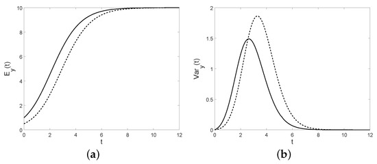Figure 13. The conditional mean (a) and the conditional variance (b) for $C=10$, $r=1$, $\sigma =1/3$ and $y=1$ (solid line), $y=0.5$ (dashed line).

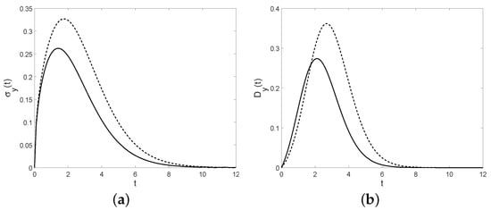Figure 14. Fano factor (a) and the coefficient of variation (b) are plotted for $C=10$, $r=1$, $\sigma =1/3$ and $y=1$ (solid line), $y=0.5$ (dashed line).

Otherwise, in the interval $I_2=(C,\infty )$, the function $\mathsf{\Phi }(x)$ is negative. Therefore the transition pdf function is

$$\begin{array}{cc}\hfill f(x,t|y)& =-\frac{1}{\sigma x\left(1-\frac{x}{C}\right)\sqrt{2\pi t}}\left[exp\left\{-\frac{1}{2{\sigma }^{2}t}{\left[log\left(\frac{x}{x-C}\right)-log\left(\frac{y}{|y-C|}\right)-rt\right]}^2\right\}\right.\hfill \\ & +\left.exp\left\{-\frac{2r}{{\sigma }^2}log\left(\frac{y}{|y-C|}\right)\right\}exp\left\{\frac{1}{2{\sigma }^{2}t}{\left[log\left(\frac{y}{|y-C|}\right)+log\left(\frac{x}{x-C}\right)-rt\right]}^2\right\}\right]\hfill \\ & +\frac{r}{{\sigma }^{2}x\left(1-\frac{x}{C}\right)}exp\left\{\frac{2r}{{\sigma }^2}log\left(\frac{x}{x-C}\right)\right\}\hfill \\ & \times \left\{1-\mathrm{Erf}\left[\frac{1}{\sigma \sqrt{2t}}\left(log\left(\frac{x}{x-C}\right)+log\left(\frac{y}{|y-C|}\right)+rt\right)\right]\right\}.\hfill \end{array}$$

(44)

Moreover, when the diffusion interval is $I_2$, if $y<S$ the first-passage-time pdf though $S\in I_2$ is

$$\begin{array}{cc}\hfill g(S,t|y)& =\frac{1}{\sigma \sqrt{2\pi t^3}}\left|log\left(\frac{S}{|S-C|}\right)-log\left(\frac{y}{|y-C|}\right)\right|\hfill \\ & \times exp\left\{-\frac{1}{2{\sigma }^{2}t}{\left[log\left(\frac{S}{|S-C|}\right)-log\left(\frac{y}{|y-C|}\right)-rt\right]}^2\right\},y<S,y\in I_2.\hfill \end{array}$$

(45)

Hence, the first-passage-time probability is given by

$$P(S|y)=\left\{\begin{array}{cc}1,\hfill & \mathrm{if}y<C\mathrm{and}S\le C\hfill \\ exp\left\{\frac{2r}{{\sigma }^2}\left[log\left(\frac{S}{|S-C|}\right)-log\left(\frac{y}{|y-C|}\right)\right]\right\},\hfill & \mathrm{if}y\ge C\mathrm{or}\left(y<C\mathrm{and}S<C\right).\hfill \end{array}\right.$$

(46)

Considering the interval $I_1=(0,C)$ and the expression of the distribution given in (41), one has that the conditional median $m\left[X(t)|X(0)=y\right]$ coincides with the solution of the deterministic logistic model, i.e.,

$$m\left[X(t)|X(0)=y\right]=\frac{Cy}{y+(C-y)e^{-rt}}.$$

Therefore, note that in both intervals, the simple paths of $X(t)$ asymptotically approach C with probability 1. We underline that for the time-inhomogeneous linear birth process analyzed in Section 4, under particular assumptions, the conditional mean is a logistic function, instead in this case the conditional median is a solution of the logistic equation.

5.2. A Time-Inhomogeneous Diffusion Process with a Conditional Logistic Mean

As shown by Román-Román and Torres-Ruiz [34], we can also look for a diffusion process with a conditional mean that is a logistic function as done for the simple birth process in Section 4. For this purpose, we consider the logistic equation written in the form (3) with the function $\xi (t)$ expressed by (5) and then we substitute the function $\xi (t)$ with $\xi (t)+\sigma B(t)$ where $B(t)$ denotes the white noise. We thus obtain

$$\frac{d\tilde{X}(t)}{dt}=\frac{r(C-y)}{y{e}^{rt}+C-y}\tilde{X}(t)+\sigma B(t)\tilde{X}(t).$$

(47)

The corresponding stochastic equation is

$$d\tilde{X}(t)=\frac{r(C-y)}{y{e}^{rt}+C-y}\tilde{X}(t)dt+\sigma \tilde{X}(t)dB(t),$$

(48)

so that its solution is a diffusion process with diffusion interval $I=(0,+\infty )$ and infinitesimal moments

$$\begin{array}{c}{\tilde{A}}_1(x,t)=\frac{r(C-y)}{y{e}^{rt}+C-y}x\hfill \\ {\tilde{A}}_2(x)={\sigma }^2{x}^2.\hfill \end{array}$$

(49)

Considering the expression of the conditional mean given in [34] and setting $b=\frac{C-y}{y}$ and $c=r$, one has that it coincides with the solution of the logistic equation. Note that this strategy is analogous to that performed in Section 4 for the logistic conditional mean of the birth process. For this reason the results about the conditional mean are the same: in both cases it corresponds to a logistic function. Moreover the transition density function is (cf. [34])

$$f(x,t|y)=\frac{1}{x\sqrt{2\pi {\sigma }^{2}t}}exp\left(-\frac{1}{2{\sigma }^{2}t}{\left[log\left(\frac{x}{y}\right)-log\left(\frac{C{e}^{rt}}{y{e}^{rt}+C-y}\right)+\frac{{\sigma }^{2}t}{2}\right]}^2\right).$$

(50)

It corresponds to a lognormal variable, i.e.,

$$\left[\tilde{X}(t)|\tilde{X}(0)=y\right]\sim \mathsf{\Lambda }\left[logy+log\left(\frac{C{e}^{rt}}{y{e}^{rt}+C-y}\right)-\frac{{\sigma }^{2}t}{2};{\sigma }^{2}t\right].$$

(51)

It follows that the variance of $\left[\tilde{X}(t)|\tilde{X}(0)=y\right]$ is given by

$$Va{r}_y(t)=Var\left[\tilde{X}(t)|\tilde{X}(0)=y\right]=\frac{C^2{y}^2\left(e^{{\sigma }^{2}t}-1\right)}{{\left(y+(C-y)e^{-rt}\right)}^2},$$

(52)

with initial value $Va{r}_y(0)=0$ and with asymptotic behavior

$$\underset{t\to \infty }{lim}Va{r}_y(t)=+\infty .$$

In Figure 15, the conditional variance $Va{r}_y(t)$ is plotted for different choices of $\sigma$.

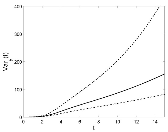
Figure 15. For $y=1$, $C=10$, $r=1$ the conditional variance $Va{r}_y(t)$ is plotted for $\sigma =1/4$ (solid line), $\sigma =1/3$ (dashed line) and $\sigma =1/5$ (dotted line). Note that it is increasing with the respect to $\sigma$.

We underline the differences between the birth process discussed in Section 4 and the diffusion process $\left\{\tilde{X}(t):t\ge 0\right\}$: in both cases, the initial value of the conditional variance is 0 but the diffusion process $\tilde{X}(t)$ is characterized by a greater variability with the respect to increasing values of t than the birth one. For the diffusion process with infinitesimal moments (49), the Fano factor has form

$$D_y(t)=\frac{Cy(e^{{\sigma }^{2}t}-1)}{y+(C-y)e^{-rt}},t\ge 0.$$

In this case, like in the simple birth process, its initial value is $D_y(0)=0$, whereas its limit is ${lim}_{t\to \infty }{D}_y(t)=+\infty$ since the conditional variance tends to infinity as $t\to \infty$. It is also increasing with the respect to C, y and $\sigma$; in particular the following limits hold:

$$\begin{array}{ccc}\underset{C\to \infty }{lim}{D}_y(t)=y{e}^{rt},\hfill & \hfill & \underset{C\to y}{lim}{D}_y(t)=y\left(e^{{\sigma }^{2}t}-1\right);\hfill \\ \underset{y\to C}{lim}{D}_y(t)=C(e^{{\sigma }^{2}t}-1),\hfill & \hfill & \underset{y\to 0}{lim}{D}_y(t)=0;\hfill \\ \underset{\sigma \to +\infty }{lim}{D}_y(t)=+\infty ,\hfill & \hfill & \underset{\sigma \to 0}{lim}{D}_y(t)=0.\hfill \end{array}$$

See Figure 16 for some comparisons between the Fano factor of the simple birth process discussed in Section 4 and of the diffusion process with infinitesimal moments (49).

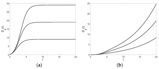
Figure 16. For $y=0.1$, $r=1$ and $\sigma =1/3$, the Fano factor $D_y(t)$ is plotted for the birth process in (a) and for the diffusion process $\tilde{X}(t)$ in (b) with $C=1,2,3$ (from bottom to top).

Recalling the expressions of the conditional mean and the conditional variance of the diffusion process $\left\{\tilde{X}(t):t\ge 0\right\}$, the coefficient of variation is given by

$${\sigma }_y(t)=\sqrt{e^{{\sigma }^{2}t}-1},t\ge 0.$$

(53)

In Figure 17, the coefficient of variation of the simple birth process analyzed in Section 4 and of the diffusion process $\tilde{X}(t)$ with infinitesimal moments (49) are plotted for some choices of the parameters.

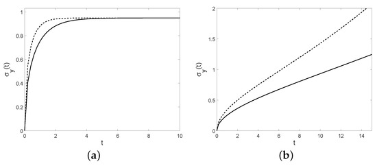
Figure 17. For $y=1$, $C=10$ the coefficient of variation ${\sigma }_y(t)$ is plotted for the birth process in (a) with $r=1$ (solid line) and $r=2$ (dashed line) and for the diffusion process in (b) with $\sigma =1/4$ (solid line) and for $\sigma =1/3$ (dashed line).

Note that in this case the coefficient of variation is independent from the choices of C and y, rather than in the simple birth process. Moreover, one has

$$\begin{array}{ccc}\underset{t\to 0}{lim}{\sigma }_y(t)=0,\hfill & \hfill & \underset{t\to \infty }{lim}{\sigma }_y(t)=+\infty \hfill \\ \underset{\sigma \to 0}{lim}{\sigma }_y(t)=0,\hfill & \hfill & \underset{\sigma \to +\infty }{lim}{\sigma }_y(t)=+\infty .\hfill \end{array}$$

In Table 7, we summarize some relevant characteristics of the simple birth process of Section 4 and of the diffusion process with infinitesimal moments (49).

Table 7. Some comparisons between the simple birth process of Section 4 and the diffusion process with infinitesimal moments (49).

Simple Birth Process	Diffusion Process $\tilde{\mathit{X}}(\mathit{t})$
$E_y(t)=\frac{Cy}{y+(C-y)e^{-rt}}$	$E_y(t)=\frac{Cy}{y+(C-y)e^{-rt}}$
$Va{r}_y(t)=\frac{Cy}{y+(C-y)e^{-rt}}\left(\frac{C}{y+(C-y)e^{-rt}}-1\right)$	$Va{r}_y(t)=\left(\frac{C^2{y}^2}{{\left(y+(C-y)e^{-rt}\right)}^2}\right)\left(e^{{\sigma }^{2}t}-1\right)$
$D_y(t)=\frac{(C-y)(e^{rt}-1)}{y{e}^{rt}+C-y}$	$D_y(t)=\frac{Cy{e}^{rt}\left(e^{{\sigma }^{2}t}-1\right)}{y{e}^{rt}+C-y}$
${\sigma }_y(t)={\left(\frac{C-y}{Cy}\right)}^{1/2}\sqrt{1-e^{-rt}}$	${\sigma }_y(t)=\sqrt{e^{{\sigma }^{2}t}-1}$

6. Diffusion in a Potential

In several applications it is useful to describe the related stochastic process as a diffusion in a potential depending on the infinitesimal moments. The original approach was developed for processes with constant infinitesimal variance (see, for instance [35]). However, since the cases considered above refer to non-constant infinitesimal variance, hereafter we adopt the transformation-based approach exploited in Section 2.3 of Di Crescenzo et al. [36]. Let us study the potentials $U(x)$ of the processes $\left\{Y(t):t\ge 0\right\}$ with infinitesimal moments (36) and $\left\{X(t):t\ge 0\right\}$ with infinitesimal moments (37). According to [36], we define the potential for a time-homogeneous diffusion process $\widehat{X}(t)$ with infinitesimal moments ${\widehat{A}}_1(x)$ and ${\widehat{A}}_2(x)$ and with state-space I as a function $U(x)$ such that

$$\frac{dU(x)}{dx}=-\frac{1}{\sqrt{{\widehat{A}}_2(x)}}\left[{\widehat{A}}_1(x)-\frac{{\widehat{A}}_2^{\prime }(x)}{4}\right],x\in I.$$

(54)

Considering the diffusion process $\{Y(t):t\ge 0\}$ with infinitesimal moments (36), one has

$$\begin{array}{c}\hfill \frac{dU(x)}{dx}=\left\{\begin{array}{cc}-\frac{r}{\sigma }+\frac{\sigma }{2}-\frac{\sigma }{C}x,\hfill & x\in (0,C)\hfill \\ +\frac{r}{\sigma }-\frac{\sigma }{2}+\frac{\sigma }{C}x,\hfill & x\in (C,+\infty ).\hfill \end{array}\right.\end{array}$$

that is a first-order ODE whose solution is

$$\begin{array}{c}\hfill U(x)=\left\{\begin{array}{cc}-\frac{r}{\sigma }x+\frac{\sigma }{2}x-\frac{\sigma }{C}{x}^2+\mathrm{const},\hfill & x\in (0,C)\hfill \\ +\frac{r}{\sigma }x-\frac{\sigma }{2}x+\frac{\sigma }{C}{x}^2+\mathrm{const},\hfill & x\in (C,+\infty ).\hfill \end{array}\right.\end{array}$$

Some plots of the potential are provided in Figure 18.

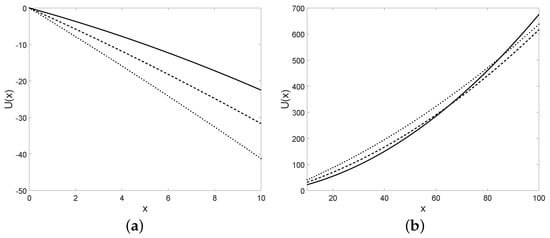
Figure 18. The potential $U(x)$ is plotted for $x\in (0,C)$ in (a) and for $x\in (C,\infty )$ in (b) and for $C=10$, $r=1$, $y=1$, $\sigma =1/2$ (solid line), $\sigma =1/3$ (dashed line), $\sigma =1/4$ (dotted line), with the initial condition $U(0)=0$.

The diffusion process $\left\{X(t):t\ge 0\right\}$, with infinitesimal moments (37) has a potential $U(x)$ such that

$$\begin{array}{c}\hfill \frac{dU(x)}{dx}=\left\{\begin{array}{cc}-\frac{r}{\sigma },\hfill & x\in (0,C)\hfill \\ +\frac{r}{\sigma },\hfill & x\in (C,+\infty )\hfill \end{array}\right.\end{array}$$

so, it is

$$U(x)=\left\{\begin{array}{cc}-\frac{r}{\sigma }x+\mathrm{const},\hfill & x\in (0,C)\hfill \\ +\frac{r}{\sigma }x+\mathrm{const},\hfill & x\in (C,+\infty ).\hfill \end{array}\right.$$

The potential is plotted for some choices of the parameters in Figure 19.

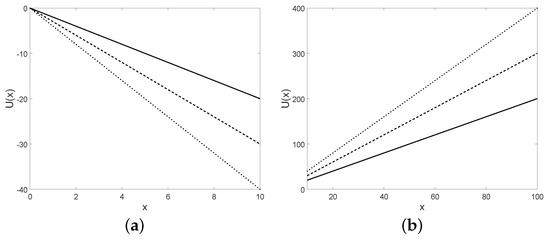
Figure 19. The potential $U(x)$ is plotted for $x\in (0,C)$ in (a) and for $x\in (C,+\infty )$ in (b) and for $C=10$, $r=1$, $y=1$ and $\sigma =1/2$ (solid line), $\sigma =1/3$ (dashed line), $\sigma =1/4$ (dotted line), with the initial condition $U(0)=0$.

Note that for the diffusion process $\left\{Y(t):t\ge 0\right\}$ with infinitesimal moments (36) the potential is a quadratic function, instead for the diffusion process $\left\{X(t):t\ge 0\right\}$ with infinitesimal moments (37) the potential is a linear function. We recall that the definition of the potential is given for regular time-homogeneous processes whose infinitesimal moments are not dependent on time. The drift ${\tilde{A}}_1(x,t)$ of the diffusion process $\left\{\tilde{X}(t):t\ge 0\right\}$ defined in Section 5.2 is dependent on time, hence the analysis of this kind of diffusion in a potential cannot be provided.

7. Conclusions

In this paper, we have considered both a deterministic logistic model and some corresponding stochastic processes.

Regarding the deterministic model, we have analyzed and compared the main characteristics of interest of the logistic model with other well-known growth models.

For the stochastic counterpart, we have paid specific attention to a time-inhomogeneous linear birth-death process which has a logistic mean. Even if the conditional mean of this process is identical to a logistic curve, it has an absorbing endpoint and this characteristic is not always appropriate to describe a growth behavior. For this reason, we have removed the possibility of downward jumps and, in this way, we have obtained a time-inhomogeneous linear simple birth process. Moreover, we have analyzed some diffusion processes obtained from the following different strategies: by approximating the logistic equation, by approximating the solution of the logistic equation and considering a different parametrization of the equation in order to have a logistic conditional mean. In Table 8, the infinitesimal moments of the analyzed diffusion processes are summarized.

Table 8. The infinitesimal moments of the diffusion processes considered in Section 5.

Model	Drift	Infinitesimal Variance
$\left\{Y(t):t\ge 0\right\}$	$A_1(x)=rx\left(1-\frac{x}{C}\right)$	$A_2(x)={\sigma }^2{x}^2{\left(1-\frac{x}{C}\right)}^2$
$\left\{X(t):t\ge 0\right\}$	$B_1(x)=rx\left(1-\frac{x}{C}\right)-\frac{1}{2}{\sigma }^{2}x\left(1-\frac{x}{C}\right)\frac{2x-C}{C}$	$B_2(x)={\sigma }^2{x}^2{\left(1-\frac{x}{C}\right)}^2$
$\left\{\tilde{X}(t):t\ge 0\right\}$	${\tilde{A}}_1(x,t)=\frac{r(C-y)}{y{e}^{rt}+C-y}x$	${\tilde{A}}_2(x)={\sigma }^2{x}^2$

Some indices of dispersion such as the Fano factor and the coefficient of variation have been determined for these processes. Finally, we have analysed the potentials for the time-homogeneous diffusion processes, reminding that diffusion processes move toward decreasing potential energy.

References

- Verhulst, P.F. Notice sur la loi que la population suit dans son accroissment. Corresp. Math. Phys. 1838, 10, 113–121. [Google Scholar]
- Tsoularis, A.; Wallace, J. Analysis of logistic growth models. Math. Biosci. 2002, 179, 21–55. [Google Scholar] [CrossRef]
- Korf, V. Prìspevek k matematickè formulaci vzrustovèho zàkona lesnìch porostu [contribution to mathematical definition of the law of stand volume growth]. Lesnickà Pràce 1939, 18, 339–379. [Google Scholar]
- Di Crescenzo, A.; Spina, S. Analysis of a growth model inspired by Gompertz and Korf laws, and an analogous birth-death process. Math. Biosci. 2016, 282, 121–134. [Google Scholar] [CrossRef]
- Pal, A.; Bhowmick, A.R.; Yeasmin, F.; Bhattacharya, S. Evolution of model specific relative growth rate: Its genesis and performance over Fisher’s growth rates. J. Theor. Biol. 2018, 444, 11–27. [Google Scholar] [CrossRef]
- Gao, X.; Wang, A.; Liu, G.; Yan, K. Expanded S-curve model of a relationship between crude steel consumption and economic development: Empiricism from case studies of developed economics. Nat. Resour. Res. 2019, 28, 547–562. [Google Scholar] [CrossRef]
- Di Crescenzo, A.; Martinucci, B.; Rhandi, A. A multispecies birth-death-immigration process and its diffusion approximation. J. Math. Anal. Appl. 2016, 442, 291–316. [Google Scholar] [CrossRef]
- Frunzo, L.; Garra, R.; Giusti, A.; Luongo, V. Modeling biological systems with an improved fractional Gompertz law. Commun. Nonlinear Sci. Num. Simul. 2019, 74, 260–267. [Google Scholar] [CrossRef]
- Di Crescenzo, A.; Martinucci, B. On a symmetric, nonlinear birth-death process with bimodal transition probabilities. Symmetry 2009, 1, 201–214. [Google Scholar] [CrossRef]
- Crawford, F.W.; Suchard, M.A. Transition probabilities for general birth-death processes with applications in ecology, genetics, and evolution. J. Math. Biol. 2012, 65, 553–580. [Google Scholar] [CrossRef]
- Bailey, N.T.J. The Elements of Stochastic Processes with Applications to the Natural Sciences; Reprint of the 1964 Original; Wiley: New York, NY, USA, 1990. [Google Scholar]
- Tan, W.Y. A stochastic Gompertz birth-death process. Stat. Prob. Lett. 1986, 4, 25–28. [Google Scholar] [CrossRef]
- Tavaré, S. The linear birth-death process: An inferential retrospective. Adv. Appl. Probab. 2018, 50, 253–269. [Google Scholar] [CrossRef]
- De Lauro, E.; De Martino, S.; De Siena, S.; Giorno, V. Stochastic roots of growth phenomena. Phys. A Stat. Mech. Its Appl. 2014, 401, 207–213. [Google Scholar] [CrossRef]
- Ricciardi, L.M. Stochastic population theory: Birth and death processes. In Mathematical Ecology; Biomathematics; Springer: Berlin/Heidelberg, Germany, 1986; Volume 17, pp. 155–190. [Google Scholar]
- Nobile, A.G.; Ricciardi, L.M. Growth with regulation in fluctuating environments. Byol. Cybern. 1984, 49, 179–188. [Google Scholar] [CrossRef]
- Nobile, A.G.; Ricciardi, L.M. Growth with regulation in fluctuating environments. II. Intrinsic lower bounds too population size. Byol. Cybern. 1984, 50, 285–289. [Google Scholar] [CrossRef]
- Román-Román, P.; Torres-Ruiz, F. The nonhomogeneous lognormal diffusion process as a general process to model particular types of growth patters. Lecture Notes of Seminario Interdisciplinare di Matematica 2015, 12, 201–219. [Google Scholar]
- Alharbi, W.; Petrovskii, S. Critical domain problem for the reaction-telegraph equation model of population dynamics. Mathematics 2018, 6, 59. [Google Scholar] [CrossRef]
- Albano, G.; Giorno, V.; Román-Román, P.; Torres-Ruiz, F. On a non-homogeneous Gompertz-type diffusion process: Inference and first passage time. EUROCAST 2017 Part II 2018, LNCS 10672, 47–54. [Google Scholar]
- Albano, G.; Giorno, V.; Román-Román, P.; Torres-Ruiz, F. Inferring the effect of therapy on tumors showing stochastic Gompertzian growth. J. Theor. Biol. 2011, 276, 67–77. [Google Scholar] [CrossRef]
- De, S.S. Stochastic model of population growth and spread. Bull. Math. Biol. 1987, 49, 1–11. [Google Scholar] [CrossRef]
- Pinheiro, S. On a logistic growth model with predation and a power-type diffusion coefficient: I. Existence of solutions and extinction criteria. Math. Methods Appl. Sci. 2015, 38, 4912–4930. [Google Scholar] [CrossRef]
- Le, V.; Pardoux, E.; Wakolbinger, A. “Trees under attack”: A Ray-Knight representation of Feller’s branching diffusion with logistic growth. Probab. Theory Relat. Fields 2013, 155, 583–619. [Google Scholar] [CrossRef]
- Hu, X. The indirect method for stochastic logistic growth models. Commun. Stat. Theory Methods 2017, 46, 1506–1518. [Google Scholar]
- Ricciardi, L.M.; Di Crescenzo, A.; Giorno, V.; Nobile, A.G. An outline of theoretical and algorithmic approaches to first passage time problems with applications to biological modeling. Math. Jpn. 1999, 50, 285–302. [Google Scholar]
- Cox, D.R.; Miller, H.D. The Theory of Stochastic Processes; Methuen: London, UK, 1970. [Google Scholar]
- Van Kampen, N.G. Itô Versus Stratonovich. J. Stat. Phys. 1981, 24, 175–187. [Google Scholar] [CrossRef]
- Braumann, C.A. Itô versus Stratonovich calculus in random population growth. Math. Biosci. 2007, 206, 81–107. [Google Scholar] [CrossRef] [PubMed]
- Braumann, C.A. Harvesting in a random environment: Itô or Stratonovich calculus? J. Theor. Biol. 2007, 244, 424–432. [Google Scholar] [CrossRef]
- Arnold, L. Stochastic Differential Equations: Theory and Applications; Wiley and Sons: New York, NY, USA, 1974. [Google Scholar]
- Feller, W. The parabolic differential equations and the associated semi-groups of transformations. Ann. Math. 1952, 55, 468–518. [Google Scholar] [CrossRef]
- Hanson, F.B.; Tier, C. An asymptotic solution of the first passage problem for singular diffusion in population biology. SIAM J. Appl. Math. 1981, 40, 113–132. [Google Scholar] [CrossRef]
- Román-Román, P.; Torres-Ruiz, F. Modelling logistic growth by a new diffusion process: Application to biological systems. BioSystems 2012, 110, 9–21. [Google Scholar] [CrossRef]
- Karlin, S.; Tayor, H.M. A Second Course in Stochastic Processes; Academic Press: New York, NY, USA, 1981. [Google Scholar]
- Di Crescenzo, A.; Giorno, V.; Nobile, A.G. Analysis of reflected diffusions via an exponential time-based transformation. J. Stat. Phys. 2016, 163, 1425–1453. [Google Scholar] [CrossRef]
© 2019 by the authors. Licensee MDPI, Basel, Switzerland. This article is an open access article distributed under the terms and conditions of the Creative Commons Attribution (CC BY) license (http://creativecommons.org/licenses/by/4.0/).