A Numerical Approximation Method for the Inverse Problem of the Three-Dimensional Laplace Equation

Abstract

In this article, an inverse problem with regards to the Laplace equation with non-homogeneous Neumann boundary conditions in a three-dimensional case is investigated. To deal with this problem, a regularization method (mollification method) with the bivariate de la Vallée Poussin kernel is proposed. Stable estimates are obtained under a priori bound assumptions and an appropriate choice of the regularization parameter. The error estimates indicate that the solution of the approximation continuously depends on the noisy data. Two experiments are presented, in order to validate the proposed method in terms of accuracy, convergence, stability, and efficiency.

1. Introduction

The inverse problem of the Laplace equation appears in many engineering and physical areas, such as geophysics, cardiology, seismology, and so on [1,2,3]. It has been widely recognized that the inverse problem for the Laplace equation has a central position in all Cauchy problems of elliptic partial differential equations. The inverse problem of the Laplace equation is seriously ill-posed, where a tiny deviation in the data can cause a large error in the solution [4]. It is difficult to develop numerical solutions with conventional methods. Some different methods have been researched, such as the quasi-reversibility [5], Tikhonov regularization [6], wavelet [7], conjugate gradient [8], central difference [9], Fourier regularization [10], and mollification [11,12,13] methods.

The main procedure of the mollification method is using the kernel function to construct a mollification operator by convolution with the measurement data. Manselli, Miller [14], and Murio [15,16] constructed mollification operators by using the Weierstrass kernel to solve some inverse heat conduction problems (IHCP). There have been reports on using the Gaussian kernel to solve the Cauchy problem of elliptic equations [17,18,19,20,21]. Hào [22,23,24] adopted the Dirichlet kernel and de la Vallée Poussin kernel to solve some kinds of two-dimensional equations; including the two-dimensional Laplace equation. However, the three-dimensional case was not considered, Moreover, the analysis method used for error estimate was does not generalize to the three-dimensional case well.

Our primary interest is to solve the inverse problem of the three-dimensional Laplace equation with non-homogeneous Neumann boundary conditions. In order to guarantee solvability for the inverse problem provided, a regularization method using the bivariate de la Vallée Poussin kernel is presented.

This paper is organized as follows: In Section 2, the mathematical problem for the three-dimensional Laplace equation and its ill-posedness are illustrated. In Section 3, we introduce the bivariate de la Vallée Poussin kernel and its properties, following which our mollification regularization method is proposed. In Section 4, some stability estimate results are given, in the interior $0<z<d$ and at the boundary $z=d$, under a priori assumptions. The numerical aspect of our proposed method is showed in Section 5. Concluding remarks are given in Section 6.

2. Mathematical Problem and the Ill-Posedness Analysis

We give thought to the following inverse problem of the three-dimensional Laplace equation with non-homogeneous Neumann boundary conditions:

$$\begin{array}{c}\hfill \left\{\begin{array}{c}\hfill ▵u(x,y,z)=0,(x,y)\in {\mathbb{R}}^2,0<z<d,\\ \hfill u(x,y,0)=g(x,y),(x,y)\in {\mathbb{R}}^2,\\ \hfill u_z(x,y,0)=h(x,y),(x,y)\in {\mathbb{R}}^2,\end{array}\right.\end{array}$$

(1)

where $\Delta =\frac{{\partial }^2}{\partial x^2}+\frac{{\partial }^2}{\partial y^2}+\frac{{\partial }^2}{\partial z^2}$ is three-dimensional Laplace operator; and $g(x,y)$, $h(x,y)$ are given vectors in $L^2({\mathbb{R}}^2)$. The solution $u(x,y,z)$ will be determined by the noisy data $g^{\delta }(x,y)$ and $h^{\delta }(x,y)$ in $L^2({\mathbb{R}}^2)$ that satisfy:

$$\parallel g-g^{\delta }{\parallel }_{L^2({\mathbb{R}}^2)}+{\parallel h-h^{\delta }\parallel }_{L^2({\mathbb{R}}^2)}\le \delta ,$$

(2)

were $\delta >0$ denotes the error level, and ${\parallel ·\parallel }_{L^2({\mathbb{R}}^2)}$ denotes the $L^2-$ norm [1].

Note that the solution of the problem (1) is the sum $u=u_1+u_2$ of the solutions for the following two problems:

$$\begin{array}{c}\hfill \left\{\begin{array}{c}\hfill ▵u_1(x,y,z)=0,(x,y)\in {\mathbb{R}}^2,0<z<d,\\ \hfill u_1(x,y,0)=g(x,y),(x,y)\in {\mathbb{R}}^2,\\ \hfill {(u_1)}_z(x,y,0)=0,(x,y)\in {\mathbb{R}}^2,\end{array}\right.\end{array}$$

(3)

and

$$\begin{array}{c}\hfill \left\{\begin{array}{c}\hfill ▵u_2(x,y,z)=0,(x,y)\in {\mathbb{R}}^2,0<z<d,\\ \hfill u_2(x,y,0)=0,(x,y)\in {\mathbb{R}}^2,\\ \hfill {(u_2)}_z(x,y,0)=h(x,y),(x,y)\in {\mathbb{R}}^2.\end{array}\right.\end{array}$$

(4)

Therefore, in order to simplify the process of the Cauchy problem (1), we only need to solve problems (3) and (4), respectively.

For $\phi \in L^2({\mathbb{R}}^2)$, the Fourier transform for a variable $\mathbf{r}=(x,y)\in {\mathbb{R}}^2$ is defined by

$$\widehat{\phi }(\xi ,z)=\frac{1}{2\pi }{\int }_{{\mathbb{R}}^2}{e}^{-i\xi ·\mathbf{r}}\phi (\mathbf{r},z)dr,$$

where $\xi =(\omega ,\eta )\in {\mathbb{R}}^2$ and $\xi ·\mathbf{r}=\omega x+\eta y$.

The inverse Fourier transform for a variable $\xi =(\omega ,\eta )\in {\mathbb{R}}^2$ is defined by

$$\phi (\mathbf{r},z)=\frac{1}{2\pi }{\int }_{{\mathbb{R}}^2}{e}^{i\xi ·\mathbf{r}}\widehat{\phi }(\xi ,z)d\xi .$$

The Parseval equality [16] is as follows:

$${\parallel \phi \parallel }_{L^2({\mathbb{R}}^2)}={\parallel \widehat{\phi }\parallel }_{L^2({\mathbb{R}}^2)}.$$

(5)

Adopting the Fourier transform for the variable $\mathbf{r}=(x,y)\in {\mathbb{R}}^2$ to problems (3) and (4), we obtain

$$\begin{array}{c}\hfill \left\{\begin{array}{c}\hfill {\widehat{(u_1)}}_{zz}=({\omega }^2+{\eta }^2)\widehat{u_1},(\omega ,\eta )\in {\mathbb{R}}^2,0<z<d,\\ \hfill \widehat{(u_1)}(\omega ,\eta ,0)=\widehat{g}(\omega ,\eta ),(\omega ,\eta )\in {\mathbb{R}}^2,\\ \hfill {\widehat{(u_1)}}_z(\omega ,\eta ,0)=0,(\omega ,\eta )\in {\mathbb{R}}^2,\end{array}\right.\end{array}$$

(6)

and

$$\begin{array}{c}\hfill \left\{\begin{array}{c}\hfill {\widehat{(u_2)}}_{zz}=({\omega }^2+{\eta }^2)\widehat{u_2},(\omega ,\eta )\in {\mathbb{R}}^2,0<z<d,\\ \hfill \widehat{(u_2)}(\omega ,\eta ,0)=0,(\omega ,\eta )\in {\mathbb{R}}^2,\\ \hfill {\widehat{(u_2)}}_z(\omega ,\eta ,0)=\widehat{h}(\omega ,\eta ),(\omega ,\eta )\in {\mathbb{R}}^2.\end{array}\right.\end{array}$$

(7)

The solution of problem (6) is

$${\widehat{u}}_1(\omega ,\eta ,z)=\widehat{g}(\omega ,\eta )\cosh (z\sqrt{{\omega }^2+{\eta }^2}).$$

(8)

Or

$$u_1(x,y,z)=\frac{1}{2\pi }{\int }_{{\mathbb{R}}^2}\widehat{g}(\omega ,\eta )\cosh (z\sqrt{{\omega }^2+{\eta }^2})e^{i\xi ·\mathbf{r}}d\xi .$$

The solution of problem (7) is

$${\widehat{u}}_2(\omega ,\eta ,z)=\widehat{h}(\omega ,\eta )\frac{\sinh (z\sqrt{{\omega }^2+{\eta }^2})}{\sqrt{{\omega }^2+{\eta }^2}}.$$

(9)

Or

$$u_2(x,y,z)=\frac{1}{2\pi }{\int }_{{\mathbb{R}}^2}\widehat{h}(\omega ,\eta )\frac{\sinh (z\sqrt{{\omega }^2+{\eta }^2})}{\sqrt{{\omega }^2+{\eta }^2}}{e}^{i\xi ·\mathbf{r}}d\xi .$$

Note that $\cosh (z\sqrt{{\omega }^2+{\eta }^2})$ and $\frac{\sinh (z\sqrt{{\omega }^2+{\eta }^2})}{\sqrt{{\omega }^2+{\eta }^2}}$ are unbounded with respect to the variable $(\omega ,\eta )$; a small perturbation in the measured data $\widehat{g}(\omega ,\eta )$ and $\widehat{h}(\omega ,\eta )$ may result in a huge deviation in the solution $u_1(x,y,z)$ and $u_2(x,y,z)$. Therefore, the problems (3) and (4) are severely ill-posed.

3. Mollification Method and Regularization Solution

3.1. Mollification Operator

The bivariate de la Vallée Poussin kernel [22] function is defined by:

$$V_{\alpha }(x,y)=\frac{(\cos (\alpha x)-\cos (2\alpha x))(\cos (\alpha y)-\cos (2\alpha y))}{{\alpha }^2{x}^2{y}^2}(\alpha >0),$$

where $\alpha >0$ is called the mollification radius (or mollification parameter). $V_{\alpha }(x,y)$ has the following properties [22]:

(1)

$V_{\alpha }(z)$ is an entire function of exponential type of degree $\alpha$ belong to $L^p({\mathbb{R}}^2)(1<p\le \infty )$;

(2)

$\frac{1}{{\pi }^2}{\int }_{{\mathbb{R}}^2}{V}_{\alpha }(x,y)dxdy=1$;

(3)

$\frac{1}{{\pi }^2}{\int }_{{\mathbb{R}}^2}|V_{\alpha }|dxdy<12(\alpha \ge 1)$; and

(4)

${\widehat{V}}_{\alpha }$ is the Fourier transform of $V_{\alpha }(x,y)$, satisfying:

$$\frac{2}{\pi }{\widehat{V}}_{\alpha }(\omega ,\eta )=1,(\omega ,\eta )\in {\Delta }_{\alpha },{\Delta }_{\alpha }:=\{|\omega |\le \alpha ,|\eta |\le \alpha \},$$

where

$${\widehat{V}}_{\alpha }(\omega ,\eta )=\upsilon (\omega )\upsilon (\eta )$$

and

$$\begin{array}{c}\hfill \upsilon (\omega )=\sqrt{\frac{\pi }{2}}\left\{\begin{array}{c}\hfill 1,|\omega |<\alpha ,\\ \hfill 2-\frac{\omega }{\alpha },\alpha <|\omega |\le 2\alpha ,\\ \hfill 0,2\alpha <|\omega |,\end{array}\right.\end{array}$$

$$\begin{array}{c}\hfill \upsilon (\eta )=\sqrt{\frac{\pi }{2}}\left\{\begin{array}{c}\hfill 1,|\eta |<\alpha ,\\ \hfill 2-\frac{\eta }{\alpha },\alpha <|\eta |\le 2\alpha ,\\ \hfill 0,2\alpha <|\eta |.\end{array}\right.\end{array}$$

For any function $D_{\alpha }\in L^1({\mathbb{R}}^2)$ and $f\in L^p({\mathbb{R}}^2)$, $1\le p\le \infty$, we define two-dimensional convolution [22] by

$$(D_{\alpha }\ast f)(x,y)=\int {\int }_{{\mathbb{R}}^2}{D}_{\alpha }(x^{\prime },y^{\prime })f(x-x^{\prime },y-y^{\prime })d{x}^{\prime }d{y}^{\prime }.$$

It is well-known that [22]

$$\widehat{(D_{\alpha }\ast f)}(\omega ,\eta )=2\pi {\widehat{D}}_{\alpha }(\omega ,\eta )\widehat{f}(\omega ,\eta )$$

(10)

and

$$\parallel D_{\alpha }{\ast f\parallel }_{L^p({\mathbb{R}}^2)}\le \parallel D_{\alpha }{\parallel }_{L^1({\mathbb{R}}^2)}{\parallel f\parallel }_{L^p({\mathbb{R}}^2)}.$$

(11)

We define the mollification operator $T_{\alpha }$ by $T_{\alpha }:{\mathbb{R}}^2\to {\mathbb{R}}^2$

$$(T_{\alpha }{g}^{\delta })(x,y)=\frac{1}{{\pi }^2}(V_{\alpha }\ast g^{\delta })(x,y),(T_{\alpha }{h}^{\delta })(x,y)=\frac{1}{{\pi }^2}(V_{\alpha }\ast h^{\delta })(x,y).$$

From (10), we have

$$\widehat{(T_{\alpha }{g}^{\delta })}(\omega ,\eta )=\frac{2}{\pi }{\widehat{V}}_{\alpha }(\omega ,\eta ){\widehat{g}}^{\delta }(\omega ,\eta ),\widehat{(T_{\alpha }{h}^{\delta })}(\omega ,\eta )=\frac{2}{\pi }{\widehat{V}}_{\alpha }(\omega ,\eta ){\widehat{h}}^{\delta }(\omega ,\eta ).$$

3.2. Regularization Approximation Solution

Instead of solving the problems (3) and (4) with the data $g^{\delta }(x,y)$ and $h^{\delta }(x,y)$, we attempt to re-construct the noisy data $g^{\delta }(x,y)$ and $h^{\delta }(x,y)$ by $(T_{\alpha }{g}^{\delta })(x,y)$ and $(T_{\alpha }{h}^{\delta })(x,y)$, respectively. We obtain the problems, with the re-constructed data, as follows:

$$\begin{array}{c}\hfill \left\{\begin{array}{c}\hfill {(u_1)}_{xx}^{\alpha ,\delta }+{(u_1)}_{yy}^{\alpha ,\delta }+{(u_1)}_{zz}^{\alpha ,\delta }=0,(x,y,z)\in \mathsf{\Omega },\\ \hfill u_1^{\alpha ,\delta }(x,y,0)=(T_{\alpha }{g}^{\delta })(x,y),(x,y)\in {\mathbb{R}}^2,\\ \hfill {(u_1)}_z^{\alpha ,\delta }(x,y,0)=0,(x,y)\in {\mathbb{R}}^2,\end{array}\right.\end{array}$$

(12)

and

$$\begin{array}{c}\hfill \left\{\begin{array}{c}\hfill {(u_2)}_{xx}^{\alpha ,\delta }+{(u_2)}_{yy}^{\alpha ,\delta }+{(u_2)}_{zz}^{\alpha ,\delta }=0,(x,y,z)\in \mathsf{\Omega },\\ \hfill u_2^{\alpha ,\delta }(x,y,0)=0,(x,y)\in {\mathbb{R}}^2,\\ \hfill {(u_2)}_z^{\alpha ,\delta }(x,y,0)=(T_{\alpha }{h}^{\delta })(x,y),(x,y)\in {\mathbb{R}}^2.\end{array}\right.\end{array}$$

(13)

The solution for problem (12) is

$${\widehat{u}}_1^{\alpha ,\delta }(\omega ,\eta ,z)=\widehat{(T_{\alpha }{g}^{\delta })}(\omega ,\eta )\cosh (z\sqrt{{\omega }^2+{\eta }^2}),$$

or

$$u_1^{\alpha ,\delta }(x,y,z)=\frac{1}{2\pi }{\int }_{{\mathbb{R}}^2}\widehat{(T_{\alpha }{g}^{\delta })}(\omega ,\eta )\cosh (z\sqrt{{\omega }^2+{\eta }^2})d\omega d\eta .$$

The solution to problem (13) is

$${\widehat{u}}_2^{\alpha ,\delta }(\omega ,\eta ,z)=\widehat{(T_{\alpha }{h}^{\delta })}(\omega ,\eta )\frac{\sinh (x\sqrt{{\omega }^2+{\eta }^2})}{\sqrt{{\omega }^2+{\eta }^2}},$$

or

$$u_2^{\alpha ,\delta }(x,y,z)=\frac{1}{2\pi }{\int }_{{\mathbb{R}}^2}\widehat{(T_{\alpha }{h}^{\delta })}(\omega ,\eta )\frac{\sinh (x\sqrt{{\omega }^2+{\eta }^2})}{\sqrt{{\omega }^2+{\eta }^2}}d\omega d\eta .$$

According to (11) and the properties (2) and (3) of the kernel $V_{\alpha }$, we have the following conclusion:

Remark 1.

If $\parallel g-g^{\delta }{\parallel }_{L^2({\mathbb{R}}^2)}\le \delta$ and $\parallel h-h^{\delta }{\parallel }_{L^2({\mathbb{R}}^2)}\le \delta$ hold, then

$$\parallel T_{\alpha }{g}^{\delta }{-g\parallel }_{L^2({\mathbb{R}}^2)}\le 12\delta ,{\parallel T_{\alpha }{h}^{\delta }-h\parallel }_{L^2({\mathbb{R}}^2)}\le 12\delta .$$

4. Parameter Selection and Error Estimates

Lemma 1.

For $z\in (0,d]$, the following inequalities hold

(1)

$\frac{\cosh (z\sqrt{{\omega }^2+{\eta }^2})}{\cosh (d\sqrt{{\omega }^2+{\eta }^2})}\le 2e^{-(d-z)\sqrt{{\omega }^2+{\eta }^2}},$

(2)

$\cosh (z\sqrt{{\omega }^2+{\eta }^2})<e^{z\sqrt{{\omega }^2+{\eta }^2}},$

(3)

$\frac{\sinh (z\sqrt{{\omega }^2+{\eta }^2})}{\sinh (d\sqrt{{\omega }^2+{\eta }^2})}\le e^{-(d-z)\sqrt{{\omega }^2+{\eta }^2}},$ and

(4)

$\frac{\sinh (z\sqrt{{\omega }^2+{\eta }^2})}{\sqrt{{\omega }^2+{\eta }^2}}<d{e}^{z\sqrt{{\omega }^2+{\eta }^2}}.$

Proof. 

Inequalities (1) and (2) are easy to obtain. From the inequalities

$$\begin{array}{cc}\hfill \frac{\sinh (z\sqrt{{\omega }^2+{\eta }^2})}{\sinh (d\sqrt{{\omega }^2+{\eta }^2})}& =\frac{e^{z\sqrt{{\omega }^2+{\eta }^2}}}{e^{d\sqrt{{\omega }^2+{\eta }^2}}}·\frac{1-e^{-2z\sqrt{{\omega }^2+{\eta }^2}}}{1-e^{-2d\sqrt{{\omega }^2+{\eta }^2}}}\hfill \\ & \le \frac{e^{z\sqrt{{\omega }^2+{\eta }^2}}}{e^{d\sqrt{{\omega }^2+{\eta }^2}}},\hfill \end{array}$$

and the Taylor expansion

$$\begin{array}{cc}\hfill \frac{\sinh (z\sqrt{{\omega }^2+{\eta }^2})}{\sqrt{{\omega }^2+{\eta }^2}}& =\sum _{n=0}^{\infty }\frac{{(\sqrt{{\omega }^2+{\eta }^2})}^{2n}{z}^{2n+1}}{(2n+1)!}\hfill \\ & \le d\sum _{n=0}^{\infty }\frac{{(z\sqrt{{\omega }^2+{\eta }^2})}^{2n}}{(2n)!}\hfill \\ & =d\cosh (z\sqrt{{\omega }^2+{\eta }^2}),\hfill \end{array}$$

we can arrive at (3) and (4). ☐

In the next content, we give stability convergence estimates between the exact solution for problems (3) and (4) and the regularization approximate solution of problems (12) and (13) in $0<z<d$ and at the boundary $z=d$, respectively. Convergence estimates will be obtained when we choose a suitable regularization parameter $\alpha$.

4.1. Error Estimates in the Interior

The convergence estimates for the proposed regularization method, in the case of $0<z<d$, will be given in this section, and we obtain the approximation results as following:

Theorem 1.

Let $u_1(x,y,z)$ and $u_1^{\alpha ,\delta }(x,y,z)$ be the exact solution and the approximation solution for problem (1) with the exact input data $g(x,y)$ and mollified data, respectively. Assume the a priori bounds $\parallel u_1{(·,·,d)\parallel }_{L^2({\mathbb{R}}^2)}\le E$ and $\parallel g-g^{\delta }{\parallel }_{L^2({\mathbb{R}}^2)}\le \delta$ hold. We have the following estimate:

$$\parallel u_1-u_1^{\alpha ,\delta }{\parallel }_{L^2({\mathbb{R}}^2)}<118E{e}^{-(d-z)\alpha }+36\delta e^{4z\alpha }.$$

(14)

If α is selected as

$$\alpha =\frac{1}{4d}\ln (E/\delta ),$$

(15)

we have

$$\parallel u_1-u_1^{\alpha ,\delta }{\parallel }_{L^2({\mathbb{R}}^2)}<118E^{(3d+z)/4d}{\delta }^{(d-z)/4d}+36E^{z/d}{\delta }^{1-z/d},$$

(16)

where E is a finite positive constant.

Proof. 

From Parseval’s equality (5) and the properties of double integrals, we have

$$\begin{array}{cc}\hfill \parallel u_1-u_1^{\alpha ,\delta }{\parallel }_{L^2({\mathbb{R}}^2)}^2& =\parallel {\widehat{u}}_1-{\widehat{u}}_1^{\alpha ,\delta }{\parallel }_{L^2({\mathbb{R}}^2)}^2=\sum _{k=1}^{25}{\int }_{D_k}{|{\widehat{u}}_1-{\widehat{u}}_1^{\alpha ,\delta }|}^{2}d\omega d\eta \hfill \\ & =\sum _{k=1}^{16}{\int }_{D_k}|\widehat{u_1}{|}^{2}d\omega d\eta +\sum _{k=17}^{25}{\int }_{D_k}{|{\widehat{u}}_1-{\widehat{u}}_1^{\alpha ,\delta }|}^{2}d\omega d\eta \hfill \\ & \le E^2\sum _{k=1}^{16}(\underset{D_k}{sup}{|A(\omega ,\eta )|)}^2+\sum _{k=17}^{25}{\int }_{D_k}{|(\widehat{g}-\widehat{(T_{\alpha }{g}^{\delta })})B(\omega ,\eta )|}^{2}d\omega d\eta .\hfill \end{array}$$

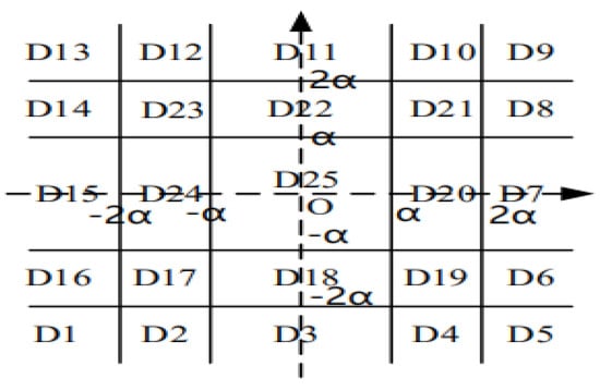
Here, ${\mathbb{R}}^2=\bigcup _{k=1}^{25}{D}_k$ (see Figure 1) and

$$A(\omega ,\eta )=\frac{\cosh (z\sqrt{{\omega }^2+{\eta }^2})}{\cosh (d\sqrt{{\omega }^2+{\eta }^2})},B(\omega ,\eta )=\cosh (z\sqrt{{\omega }^2+{\eta }^2}),(\omega ,\eta \in \mathbb{R}).$$

Figure 1. For every $D_k(k=1,2,\cdots ,25)$

Furthermore,

$$\begin{array}{c}\sum _{k=17}^{25}{\int }_{D_k}{|(\widehat{g}-\widehat{(T_{\alpha }{g}^{\delta })})B(\omega ,\eta )|}^{2}d\omega d\eta =\hfill \\ {\int }_{D_{17}}|(\widehat{g}-(2-\frac{\omega }{\alpha })(2-\frac{\eta }{\alpha }){\widehat{g}}^{\delta })B(\omega ,\eta ){|}^{2}d\omega d\eta +{\int }_{D_{18}}{|(\widehat{g}-(2-\frac{\eta }{\alpha }){\widehat{g}}^{\delta })B(\omega ,\eta )|}^{2}d\omega d\eta +\hfill \\ {\int }_{D_{19}}|(\widehat{g}-(2-\frac{\omega }{\alpha })(2-\frac{\eta }{\alpha }){\widehat{g}}^{\delta })B(\omega ,\eta ){|}^{2}d\omega d\eta +{\int }_{D_{20}}{|(\widehat{g}-(2-\frac{\omega }{\alpha }){\widehat{g}}^{\delta })B(\omega ,\eta )|}^{2}d\omega d\eta +\hfill \\ {\int }_{D_{21}}|(\widehat{g}-(2-\frac{\omega }{\alpha })(2-\frac{\eta }{\alpha }){\widehat{g}}^{\delta })B(\omega ,\eta ){|}^{2}d\omega d\eta +{\int }_{D_{22}}{|(\widehat{g}-(2-\frac{\eta }{\alpha }){\widehat{g}}^{\delta })B(\omega ,\eta )|}^{2}d\omega d\eta +\hfill \\ {\int }_{D_{23}}|(\widehat{g}-(2-\frac{\omega }{\alpha })(2-\frac{\eta }{\alpha }){\widehat{g}}^{\delta })B(\omega ,\eta ){|}^{2}d\omega d\eta +{\int }_{D_{24}}{|(\widehat{g}-(2-\frac{\omega }{\alpha }){\widehat{g}}^{\delta })B(\omega ,\eta )|}^{2}d\omega d\eta +\hfill \\ {\int }_{D_{25}}{|(\widehat{g}-{\widehat{g}}^{\delta })B(\omega ,\eta )|}^{2}d\omega d\eta .\hfill \end{array}$$

It is easy to verify that $9<(2-\frac{\omega }{\alpha })(2-\frac{\eta }{\alpha })<16,(\omega ,\eta )\in D_{17}$,

$$D_{17}=(-2\alpha ,-\alpha )\times (-2\alpha ,-\alpha ).$$

From Minkowski’s inequality, we have

$$\begin{array}{c}({\int }_{D_{17}}|(\widehat{g}-(2-\frac{\omega }{\alpha })(2-\frac{\eta }{\alpha }){\widehat{g}}^{\delta })B(\omega ,\eta ){{|}^{2}d\omega d\eta )}^{1/2}\hfill \\ =\parallel (\widehat{g}-(2-\frac{\omega }{\alpha })(2-\frac{\eta }{\alpha }){\widehat{g}}^{\delta })B(\omega ,\eta ){\parallel }_{L^2(D_{17})}\hfill \\ \le \parallel \widehat{g}{B(\omega ,\eta )\parallel }_{L^2(D_{17})}+16{\parallel ({\widehat{g}}^{\delta }-\widehat{g}+\widehat{g})B(\omega ,\eta )\parallel }_{L^2(D_{17})}\hfill \\ \le 17\parallel \widehat{g}{B(\omega ,\eta )\parallel }_{L^2(D_{17})}+16{\parallel ({\widehat{g}}^{\delta }-\widehat{g})B(\omega ,\eta )\parallel }_{L^2(D_{17})}\hfill \\ \le 17E\underset{D_{17}}{sup}|A(\omega ,\eta )|+16\delta \underset{D_{17}}{sup}|B(\omega ,\eta )|.\hfill \end{array}$$

Using a similar analysis, we can obtain the integral estimates of the other $D_k(k=18,\cdots ,24)$.

Utilizing the inequality $\sqrt{A+B+C}<\sqrt{A}+\sqrt{B}+\sqrt{C}(A>0,B>0,C>0)$, we have

$$\begin{array}{c}\parallel u_1-u_1^{\alpha ,\delta }{\parallel }_{L^2({\mathbb{R}}^2)}={\parallel {\widehat{u}}_1-{\widehat{u}}_1^{\alpha ,\delta }\parallel }_{L^2({\mathbb{R}}^2)}\hfill \\ \le E\sum _{k=1}^{16}\underset{D_k}{sup}|A(\omega ,\eta )|+\sum _{k=17}^{25}({\int }_{D_k}|(\widehat{g}-\widehat{(T_{\alpha }{g}^{\delta })})B(\omega ,\eta ){{|}^{2}d\omega d\eta )}^{1/2}.\hfill \end{array}$$

According to (1) and (2) of Lemma 1, we obtain

$$\begin{array}{c}\parallel u_1-u_1^{\alpha ,\delta }{\parallel }_{L^2({\mathbb{R}}^2)}\le 2E(4e^{-2\sqrt{2}(d-z)\alpha }+8e^{-\sqrt{5}(d-z)\alpha }+4e^{-2(d-z)\alpha })+\hfill \\ (34E{e}^{-(d-z)\sqrt{2}\alpha }+16\delta e^{2\sqrt{2}z\alpha })+(10E{e}^{-(d-z)\alpha }+4\delta e^{\sqrt{5}z\alpha })+(10E{e}^{-(d-z)\sqrt{2}\alpha }+4\delta e^{2\sqrt{2}z\alpha })+\hfill \\ (4E{e}^{-(d-z)\alpha }+\delta e^{\sqrt{5}z\alpha })+(4E{e}^{-(d-z)\sqrt{2}\alpha }+\delta e^{2\sqrt{2}z\alpha })+(4E{e}^{-(d-z)\alpha }+\delta e^{\sqrt{5}z\alpha })+\hfill \\ (10E{e}^{-(d-z)\sqrt{2}\alpha }+4\delta e^{2\sqrt{2}z\alpha })+(10E{e}^{-(d-z)\alpha }+4\delta e^{\sqrt{5}z\alpha })+\delta e^{\sqrt{2}z\alpha }\hfill \\ \le 118E{e}^{-(d-z)\alpha }+36\delta e^{2\sqrt{2}z\alpha }\hfill \\ <118E{e}^{-(d-z)\alpha }+36\delta e^{4z\alpha }.\hfill \end{array}$$

Taking parameter $\alpha$ to be $\alpha =\frac{1}{4d}\ln (E/\delta )$, we arrive at (16). ☐

Similarly, the error estimate for problem (4) can be obtained in the following way.

Theorem 2.

Let $u_2(x,y,z)$ and $u_2^{\alpha ,\delta }(x,y,z)$ be the exact solution and approximation solution for problem (4) with the exact input data $h(x,y)$ and mollified data, respectively. Assume that the a priori bounds $\parallel u_2{(·,·,d)\parallel }_{L^2({\mathbb{R}}^2)}\le E$ and $\parallel h-h^{\delta }{\parallel }_{L^2({\mathbb{R}}^2)}\le \delta$ hold, we have

$$\parallel u_2-u_2^{\alpha ,\delta }{\parallel }_{L^2({\mathbb{R}}^2)}<59E{e}^{-(d-z)\alpha }+36d\delta e^{4z\alpha }.$$

(17)

If α is chosen as in (15), then we have

$$\parallel u_2-u_2^{\alpha ,\delta }{\parallel }_{L^2({\mathbb{R}}^2)}<59E^{(3d+z)/4d}{\delta }^{(d-z)/4d}+36d{E}^{z/d}{\delta }^{1-z/d}.$$

(18)

As for our problem (1), combining the results of Theorems 1 and 2 and the Minkowski inequality, we have the error estimate, as follows:

Theorem 3.

Let $u(x,y,z)$ and $u^{\alpha ,\delta }(x,y,z)$ be the exact solution and regular solution for problem (1). Assume that condition (2) and $max\{\parallel u_1(·,·,d){\parallel }_{L^2({\mathbb{R}}^2)},\parallel u_2(·,·,d){\parallel }_{L^2({\mathbb{R}}^2)}\}\le E$ hold. Then, we have

$$\parallel u-u^{\alpha ,\delta }{\parallel }_{L^2({\mathbb{R}}^2)}<177E{e}^{-(d-z)\alpha }+36(d+1)\delta e^{4z\alpha }.$$

(19)

If α is chosen as in (15), then we have

$$\parallel u-u^{\alpha ,\delta }{\parallel }_{L^2({\mathbb{R}}^2)}<177E^{(3d+z)/4d}{\delta }^{(d-z)/4d}+36(d+1)E^{z/d}{\delta }^{1-z/d}.$$

(20)

4.2. Error Estimates at the Boundary

The estimates (14), (17), and (19) give no information about the error estimates at $z=d$, as the constraints $\parallel u_1{(·,·,d)\parallel }_{L^2({\mathbb{R}}^2)}\le E$ and $\parallel u_2{(·,·,d)\parallel }_{L^2({\mathbb{R}}^2)}\le E$ are too weak for this purpose. Therefore, to ensure stability of the solution $u_1(x,y,z)$, $u_2(x,y,z)$ at $z=d$, we need the Sobolev space $H^p({\mathbb{R}}^2)$$(p\ge 0)$ [1],

$$H^p({\mathbb{R}}^2)=\{\phi (x,y)\in L^2({\mathbb{R}}^2){:\parallel \phi \parallel }_{H^p({\mathbb{R}}^2)}<\infty \},$$

where ${\parallel ·\parallel }_{H^p({\mathbb{R}}^2)}$ is defined by

$${\parallel \phi (·,·,d)\parallel }_{H^p({\mathbb{R}}^2)}={\parallel {(1+{\omega }^2+{\eta }^2)}^{p/2}\widehat{\phi }(\omega ,\eta ,d)\parallel }_{L^2({\mathbb{R}}^2)}.$$

If $p=0$, then $H^0=L^2({\mathbb{R}}^2)$.

Theorem 4.

Let $u_1(x,y,d)$ and $u_1^{\alpha ,\delta }(x,y,d)$ be the exact and regularization solutions, respectively, of problem (3) at $z=d$. Suppose that the a priori bounds $\parallel u_1{(·,·,d)\parallel }_{H^p({\mathbb{R}}^2)}\le E_p$$(p>0)$ and $\parallel g-g^{\delta }{\parallel }_{L^2({\mathbb{R}}^2)}\le \delta$ hold. Then, we have the following inequality

$$\parallel u_1(·,·,d)-u_1^{\alpha ,\delta }{(·,·,d)\parallel }_{L^2({\mathbb{R}}^2)}<\frac{59E_p}{{(1+{\alpha }^2)}^{p/2}}+36\delta e^{4d\alpha }.$$

(21)

If the regular parameter α is selected as

$$\alpha =\frac{1}{8d}\ln (E_p/\delta ),$$

(22)

then we have

$$\parallel u_1(·,·,d)-u_1^{\alpha ,\delta }{(·,·,d)\parallel }_{L^2({\mathbb{R}}^2)}<59E_p{(\frac{8d}{\ln (E_p/\delta )})}^p+36E_p^{1/2}{\delta }^{1/2},$$

(23)

where $E_p$ is a positive constant only depending on p.

Proof. 

From Parseval’s equality (5), we have

$$\begin{array}{c}\parallel u_1(·,·,d)-u_1^{\alpha ,\delta }{(·,·,d)\parallel }_{L^2({\mathbb{R}}^2)}^2={\parallel \widehat{u_1}(·,·,d)-{\widehat{u_1}}^{\alpha ,\delta }(·,·,d)\parallel }_{L^2({\mathbb{R}}^2)}^2\hfill \\ =\sum _{k=1}^{25}\int {\int }_{D_k}{|\widehat{u_1}(·,·,d)-{\widehat{u_1}}^{\alpha ,\delta }(·,·,d)|}^{2}d\omega d\eta \hfill \\ =\sum _{k=1}^{16}\int {\int }_{D_k}|\widehat{u}{(·,·,d)|}^{2}d\omega d\eta +\sum _{k=17}^{25}\int {\int }_{D_k}{|\widehat{u_1}(·,·,d)-{\widehat{u_1}}^{\alpha ,\delta }(·,·,d)|}^{2}d\omega d\eta ,\hfill \end{array}$$

where $D_k(k=1,2,\cdots ,25)$ are same as in Theorem 1. Let

$$R(\omega ,\eta )=\frac{1}{{(1+{\omega }^2+{\eta }^2)}^{p/2}}(\omega ,\eta \in \mathbb{R}).$$

Using the properties of the double integral, and the inequality $\sqrt{A+B+C}<\sqrt{A}+\sqrt{B}+\sqrt{C}(A>0,B>0,C>0)$, we have

$$\begin{array}{c}\parallel u_1(·,·,d)-u_1^{\alpha ,\delta }{(·,·,d)\parallel }_{L^2({\mathbb{R}}^2)}\hfill \\ \le E\sum _{k=1}^{16}\underset{D_k}{sup}|R(\omega ,\eta )|+\sum _{k=17}^{25}(\int {\int }_{D_k}|\widehat{u_1}(·,·,d)-{\widehat{u_1}}^{\alpha ,\delta }(·,·,d){{|}^{2}d\omega d\eta )}^{1/2}.\hfill \end{array}$$

Using a similar method as in Theorem 1 and the monotonicity of the function $R(\omega ,\eta )$, we obtain

$$\begin{array}{cc}\hfill \parallel u_1(·,·,d)-u_1^{\alpha ,\delta }{(·,·,d)\parallel }_{L^2({\mathbb{R}}^2)}& <\frac{59E_p}{{(1+{\alpha }^2)}^{p/2}}+36\delta e^{4d\alpha }.\hfill \end{array}$$

If we chose $\alpha$ as $\alpha =\frac{1}{8d}\ln (E_p/\delta )$ and utilize inequality $1+{\alpha }^2>{\alpha }^2$, then (23) can be obtained. ☐

Similar to Theorem 4, the error estimate for problem (4) can be obtained as follows.

Theorem 5.

Let $u_2(x,y,d)$ and $u_2^{\alpha ,\delta }(x,y,d)$ be the exact and regularization solutions, respectively, for problem (4) at $z=d$. Suppose that the a priori bounds $\parallel u_2{(·,·,d)\parallel }_{H^p({\mathbb{R}}^2)}\le E_p$ and $\parallel h-h^{\delta }{\parallel }_{L^2({\mathbb{R}}^2)}\le \delta$ hold. Then, we have the following inequality

$$\parallel u_2(·,·,d)-u_2^{\alpha ,\delta }{(·,·,d)\parallel }_{L^2({\mathbb{R}}^2)}<\frac{59E_p}{{(1+{\alpha }^2)}^{p/2}}+36d\delta e^{4d\alpha }.$$

(24)

If the regularization parameter α is chosen as in (22), then

$$\parallel u_2(·,·,d)-u_2^{\alpha ,\delta }{(·,·,d)\parallel }_{L^2({\mathbb{R}}^2)}<59E_p{(\frac{8d}{\ln (E_p/\delta )})}^p+36d{E}_p^{1/2}{\delta }^{1/2}.$$

(25)

Thus, as for problem (1), using the results of Theorems 4 and 5 and the Minkowski inequality, we have the stable error estimate, as follows:

Theorem 6.

Let $u(x,y,d)$ and $u^{\alpha ,\delta }(x,y,d)$ be the exact and regularization solutions, respectively, for problem (1) at $z=d$. Suppose that condition (2) and $max\{\parallel u_1{(·,·,d)\parallel }_{H^p({\mathbb{R}}^2)},\parallel u_2(·,·,d){\parallel }_{H^p({\mathbb{R}}^2)}\}\le E_p$$(p>0)$ hold. We have the convergence estimate, as follows:

$$\parallel u(·,·,d)-u^{\alpha ,\delta }{(·,·,d)\parallel }_{L^2({\mathbb{R}}^2)}<\frac{118E_p}{{(1+{\alpha }^2)}^{p/2}}+36(d+1)\delta e^{4d\alpha }.$$

(26)

If the regularization parameter α is selected as in (22), then

$$\parallel u(·,·,d)-u^{\alpha ,\delta }{(·,·,d)\parallel }_{L^2({\mathbb{R}}^2)}<118E_p{(\frac{8d}{\ln (E_p/\delta )})}^p+36(d+1)E_p^{1/2}{\delta }^{1/2}.$$

(27)

Remark 2.

In this part, we consider the stable error estimates in the cases $0<z<d$ and $z=d$, respectively. In the interior, $0<z<d$, the a priori bound for ${\parallel u(·,·,d)\parallel }_{L^2({\mathbb{R}}^2)}$ is sufficient, and the convergence estimate converges quickly to zero as $\delta \to 0^{+}$. However, for the case $z=d$, although a stronger a priori bound for ${\parallel u(·,·,d)\parallel }_{H^p({\mathbb{R}}^2)}(p>0)$ is imposed, the error estimate is only of logarithmic type, with order ${(\ln (E_p/\delta ))}^{-p}(p>0)$.

5. Numerical Examples

We performed two numerical examples to verify the accuracy and stability of our proposed method. Our tests were carried out in the MATLAB R2014b software.

In the numerical examples, we selected the discrete interval to be $D=[-6-\gamma ,6+\gamma ]\times [-6-\gamma ,6+\gamma ](\gamma =1\times {10}^{-3})$ and the measurement data ${\varphi }^{\delta }(x,y)$ was obtained as the following

$${\varphi }^{\delta }(x,y)=\varphi +ϵ(2randn(size(\varphi ))-1),$$

where

$$\varphi ={(\varphi (x_i,y_j))}_{N\times N},x_i=-6+\frac{12(i-1)}{N-1},y_j=-6+\frac{12(j-1)}{N-1},i,j=1,2,\cdots ,N.$$

The error level $\delta$ is given by

$$\delta =\parallel \varphi -{\varphi }^{\delta }{\parallel }_{l^2(D)}=\sqrt{\frac{1}{N\times N}\sum _{i=1}^N\sum _{j=1}^N{(\varphi (x_i,y_j)-{\varphi }^{\delta }(x_i,y_j))}^2}.$$

In the following numerical implementations, we need to take the two-dimensional discrete Fourier transform of the data vector ${\varphi }^{\delta }(x,y)$ and the two-dimensional discrete inverse Fourier transform. We take $d=1$, $N=15$, and fix the reconstructed position $z=0.3$. The a priori mollification parameter $\alpha$ was determined by (15) and (22), where ${\parallel \phi (·,·,d)\parallel }_{l^2(D)}=E$ and ${\parallel \phi (·,·,d)\parallel }_{H^p(D)}=E_p$. We define the relative error between the exact solution u and its approximate solution $u^{\alpha ,\delta }$ as:

$$rel(u)=\frac{\parallel u-u^{\alpha ,\delta }{\parallel }_{l^2(D)}}{{\parallel u\parallel }_{l^2(D)}}.$$

Example 1.

We chose the function $g(x,y)=xy{e}^{-x^2-y^2}$ as the exact data for problem (3).

Example 2.

We chose the function $h(x,y)=e^{-\frac{36}{36+x^2}-\frac{36}{36+y^2}}$ as the exact data for problem (4).

We use different perturbation noise levels at the boundary $z=1$ with $p=0.5$ and $p=3$, respectively, in Table 1 and Table 2. Note that the results for the relative error $rel(u)$ at $z=1$ depended on the error level, $\delta$, and p.

Table 1. Example 1: Relative Error at $z=1$, $p=0.5$ and $p=3$.

p	Error Level $\mathit{\delta }$	Regular Parameter $\mathit{\alpha }$	Relative Error $\mathit{rel}(\mathit{u})$
0.5	$1\times {10}^{-8}$	5.3392	0.2764
0.5	$1\times {10}^{-9}$	5.9148	0.0955
3	$1\times {10}^{-7}$	5.8034	0.1363
3	$1\times {10}^{-8}$	6.3790	0.0777

Table 2. Example 2: Relative Error at $z=1$, $p=0.5$ and $p=3$.

p	Error Level $\mathit{\delta }$	Regular Parameter $\mathit{\alpha }$	Relative Error $\mathit{rel}(\mathit{u})$
0.5	$1\times {10}^{-8}$	5.4041	0.2404
0.5	$1\times {10}^{-9}$	5.9798	0.0509
3	$1\times {10}^{-6}$	5.2927	0.2684
3	$1\times {10}^{-7}$	10.6332	0.0905

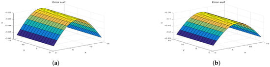
Figure 2 and Figure 3 show the re-constructed solution and exact solution of Example 1, corresponding to noise levels of $\delta =1\times {10}^{-10}$ and $\delta =2\times {10}^{-8}$, with $z=0.3$ and $z=1$, respectively. Figure 4 shows the corresponding error between (a) and (b) in Figure 2 and Figure 3.

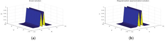
Figure 2. Example 1: $\delta =1\times {10}^{-10}$, $z=0.3$: (a) Exact solution, and (b) approximation solution.

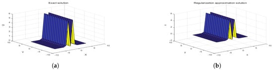
Figure 3. Example 1: For $\delta =2\times {10}^{-8}$, $z=1$: (a) Exact solution, and (b) approximation solution.

Figure 4. Example 1: (a) The error between (a) and (b) in Figure 2, and (b) the error between (a) and (b) in Figure 3.

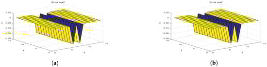
Figure 5 and Figure 6 show the regularization solution and exact solution of Example 2, corresponding to noise levels of $\delta =1\times {10}^{-10}$ and $\delta =2\times {10}^{-8}$ with $z=0.3$ and $z=1$, respectively. Figure 7 shows the corresponding error between (a) and (b) in Figure 5 and Figure 6.

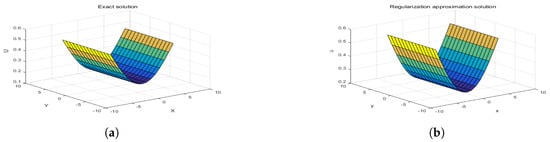
Figure 5. Example 2: $\delta =1\times {10}^{-10}$, $z=0.3$: (a) Exact solution, and (b) approximation solution.

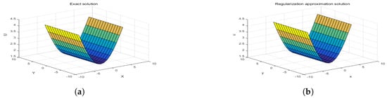
Figure 6. Example 2: For $\delta =2\times {10}^{-8}$, $z=1$: (a) Exact solution, and (b) approximation solution.

Figure 7. Example 2: (a) The error between (a) and (b) in Figure 5, and (b) the error between (a) and (b) in Figure 6.

In the two examples, we note that the methods which we adopted are stable and effective.

6. Conclusions

In this article, we use a regularization method to solve two Cauchy problems for the three-dimensional Laplace equation. Stable approximate estimates are obtained under a priori bound assumptions and an appropriate choice of the regular parameter. Two numerical examples are investigated to verify the stability of our presented method.

We consider stability error estimates in the cases $0<z<d$ and $z=d$, respectively. In the interior, $0<z<d$, the convergence estimate is $O({\delta }^{\lambda })$$(\lambda >0)$, which quickly converges to zero as $\delta \to 0^{+}$. However, at the boundary, $z=d$, the error estimate is of logarithmic type with order ${(\ln (E_p/\delta ))}^{-p}(p>0)$. In future work, we hope to find a new a priori assumption method, in order to obtain an error estimation which achieves better results.

References

- Tikhonov, A.N.; Arsenin, V.Y. Solutions of Ill-Posed Problems; Winson: Washington, DC, USA, 1977; pp. 10–80. [Google Scholar]
- Colli-Franzone, P.; Magenes, E. On the inverse potential problem of electrocardiology. Calcolo 1980, 10, 459–538. [Google Scholar]
- Alessandrini, G. Stable determination of a crack from boundary measurements. Proc. R. Soc. Edinb. 1993, 123, 497–516. [Google Scholar] [CrossRef]
- Hadamard, J. Lectures on the Cauchy Problem in Linear Partial Differential Equations; Yale University Press: New Haven, CT, USA, 1923. [Google Scholar]
- Klibanov, M.V.; Santosa, F. A computational quasi-reversibility method for Cauchy problems for Laplace equation. SIAM J. Appl. 1991, 56, 1653–1675. [Google Scholar] [CrossRef]
- Reinhardt, H.J.; Han, H.; Hào, D.N. Stability and regularization of a discrete approximation to the Cauchy problem for Laplace’s equation. SIAM J. Numer. Anal. 1999, 36, 890–905. [Google Scholar] [CrossRef]
- Wang, W.F.; Wang, J.R. Wavelet solution to the three-Dimensional Cauchy problem for Laplace equation. J. Math. 2012, 36, 239–248. [Google Scholar]
- Hào, D.N.; Lesnic, D. The Cauchy problem for Laplace’s equation via the conjugate gradient method. IMA J. Appl. Math. 2000, 65, 199–217. [Google Scholar] [CrossRef]
- Xiong, X.T.; Fu, C.L. Central difference regularization method for the Cauchy problem of the Laplace’s equation. Appl. Math. Comput. 2006, 181, 675–684. [Google Scholar] [CrossRef]
- Fu, C.L.; Li, H.F.; Qian, Z.; Xiong, X.T. Fourier regularization method for solving a Cauchy problem for the Laplace equation. Inverse Probl. Sci. Eng. 2008, 16, 159–169. [Google Scholar] [CrossRef]
- Li, Z.P.; Fu, C.L. A mollification method for a Cauchy problem for the Laplace equation. Appl. Math. Comput. 2011, 217, 9209–9218. [Google Scholar] [CrossRef]
- Ang, D.D.; Nghia, N.H.; Tam, N.C. Regularized solutions of a Cauchy Problem for Laplace Equation in an irregular layer: A three dimensional model. Acta Math. Vietnam. 1998, 23, 65–74. [Google Scholar]
- Cheng, J.; Hon, Y.C.; Wei, T.; Yamamoto, M. Numerical computation of a Cauchy Problem for Laplace’s equation. Zammz. Angew. Math. Mech. 2001, 81, 665–674. [Google Scholar] [CrossRef]
- Manselli, P.; Miller, K. Calculation of the surface temperature and heat flux on one side of a wall from measurements on the opposite side. Ann. Mat. Pura Appl. 1980, 123, 161–183. [Google Scholar] [CrossRef]
- Murio, D.A. Numerical method for inverse transient heat conduction problems. Rev. De La Unión Matemátic Argentina 1981, 30, 25–46. [Google Scholar]
- Murio, D.A. On the estimation of the boundary temperature on a sphere from measurements at its center. J. Comp. Appl. Math. 1982, 8, 111–119. [Google Scholar] [CrossRef]
- Hao, C.; Li, F.X.; Fu, C.L. A mollification regularization method for the Cauchy problem of an elliptic equation in a multi-dimensional case. Inverse Probl. Sci. Eng. 2010, 18, 971–982. [Google Scholar]
- Xiong, X.T.; Shi, W.X.; Fan, X.Y. Two numerical methods for a Cauchy problem for modified Helmholtz equation. Appl. Math. Model. 2011, 35, 4915–4920. [Google Scholar] [CrossRef]
- Yang, F.; Fu, C.L.; Li, X.X. A mollification regularization method for identifying the time-dependent heat source problem. J. Eng. Math. 2016, 100, 67–80. [Google Scholar] [CrossRef]
- Xiong, X.T.; Mao D, L.; Cao, X.X. A mollification method for solving the Cauchy problem for the modified Helmholtz equation. J. Northwest Univ. (Nat. Sci.) 2018, 53, 1–7. [Google Scholar]
- Ern, A.; Guermond, J.L. Mollification in strongly Lipschitz domains with application to continuous and discrete de Rham complexes. Comput. Methods Appl. Math. 2016, 16, 51–75. [Google Scholar] [CrossRef]
- Hào, D.N. A mollification method for ill-posed problems. Numer. Math. 1994, 68, 469–506. [Google Scholar]
- Hào, D.N. A mollification method for a Noncharacteristic Cauchy Problem for a Parabolic Equation. Math. Anal. Appl. 1996, 199, 873–909. [Google Scholar] [CrossRef]
- Hào, D.N.; Hien, P.M.; Sahli, H. Stability results for a Cauchy problem for an elliptic equation. Inverse Probl. 2007, 23, 421–461. [Google Scholar] [CrossRef]
© 2019 by the authors. Licensee MDPI, Basel, Switzerland. This article is an open access article distributed under the terms and conditions of the Creative Commons Attribution (CC BY) license (http://creativecommons.org/licenses/by/4.0/).