An Efficient Memetic Algorithm for the Minimum Load Coloring Problem

Abstract

Given a graph G with n vertices and l edges, the load distribution of a coloring q: V → {red, blue} is defined as d_q = (r_q, b_q), in which r_q is the number of edges with at least one end-vertex colored red and b_q is the number of edges with at least one end-vertex colored blue. The minimum load coloring problem (MLCP) is to find a coloring q such that the maximum load, l_q = 1/l × max{r_q, b_q}, is minimized. This problem has been proved to be NP-complete. This paper proposes a memetic algorithm for MLCP based on an improved K-OPT local search and an evolutionary operation. Furthermore, a data splitting operation is executed to expand the data amount of global search, and a disturbance operation is employed to improve the search ability of the algorithm. Experiments are carried out on the benchmark DIMACS to compare the searching results from memetic algorithm and the proposed algorithms. The experimental results show that a greater number of best results for the graphs can be found by the memetic algorithm, which can improve the best known results of MLCP.

1. Introduction

The minimum load coloring problem (MLCP) of the graph, discussed in this paper, was introduced by Nitin Ahuja et al. [1]. This problem is described as follows: a graph G = (V, E) is given, in which V is a set of n vertices, and E is a set of l edges. The load of a k-coloring $\phi$: V → {1, 2, 3,…,k} is defined as

$$1/l\times \underset{i\in \{1,2,3\dots ,k\}}{\max }|\{e\in E|{\phi }^{-1}(i)\cap e\ne \varnothing \}|,$$

the maximum fraction of edges with at least one end-point in color i, where the maximum is taken over all i ∈ {1,2,3,…,k}. The aim of the minimum load coloring problem is to minimize the load over all k-colorings.

This paper is dedicated to the NP-complete minimum load coloring problem [1]. We focus on coloring the vertices with the colors of red and blue. A graph G = (V, E) is given, in which V is a set of n vertices, and E is a set of l edges. The load distribution of a coloring q: V → {red, blue} is defined as d_q = (r_q, b_q), in which r_q is the number of edges with at least one end-vertex colored red, and b_q is the number of edges with at least one end-vertex colored blue. The objective of MLCP is to find a coloring q such that the maximum load, l_q = 1/l × max{r_q, b_q}, is minimized. MLCP can be applied to solve the wavelength division multiplexing (WDM) problem of network communication, and build the WDM network and complex power network [1,2,3].

This paper proposes an effective memetic algorithm for the minimum load coloring problem, which relies on four key components. Firstly, an improved K-OPT local search procedure, combining a tabu search strategy and a vertices addition strategy, is especially designed for MLCP to explore the search space and escape from the local optima. Secondly, a data splitting operation is used to expand the amount of data in the search space, which enables the memetic algorithm to explore in a larger search space. Thirdly, to find better global results, through randomly changing the current search patterns a disturbance operation is employed to improve the probability of escaping from the local optima. Finally, a population evolution mechanism is devised to determine how the better solution is inserted into the population.

We evaluate the performance of memetic algorithm on 59 well-known graphs from benchmark DIMACS coloring competitions. The computational results show that the search ability of memetic algorithm is better than those of simulated annealing algorithm, greedy algorithm, artificial bee colony algorithm [4] and variable neighborhood search algorithm [5]. In particular, it improves the best known results of 16 graphs in known literature algorithms.

The paper is organized as follows. Section 2 describes the related work of heuristic algorithms. Section 3 describes the general framework and the components of memetic algorithm, including the population initialization, the data splitting operation, the improved K-OPT local search procedure of individuals, the evolutionary operation and the disturbance operation. Section 4 describes the design process of simulated annealing algorithm. Section 5 describes the design process of greedy algorithm. Section 6 describes the experimental results. Section 7 describes the conclusion of the paper.

2. Related Work

In [6,7], the parameterized and approximation algorithms are proposed to solve the load coloring problem, and theoretically prove their capability in finding the best solution. On the other hand, considering the theoretical intractability of MLCP, several heuristic algorithms are proposed to find the best solutions. Heuristic algorithms use rules based on previous experience to solve a combinatorial optimization problem at the cost of acceptable time and space, and, at the same time, comparatively better results can be obtained. The heuristic algorithms used here include an artificial bee colony algorithm [4], a tabu search algorithm [5] and a variable neighborhood search algorithm [5] to solve MLCP.

Furthermore, to find the best solutions of the other combinatorial optimization problems, several heuristic algorithms are employed, such as a variable neighborhood search algorithm [8,9], a tabu search algorithm [10,11,12,13], a simulated annealing algorithm [14,15,16,17], and a greedy algorithm [18].

Local search algorithm, as an important heuristic algorithm, has been improved and evolved into many updated forms, such as a variable depth search algorithm [19], a reactive local search algorithm [20], an iterated local search algorithm [21], and a phased local search algorithm [22].

Memetic algorithm [23,24] is an optimization algorithm which combines population-based global search and individual-based local heuristic search, whose application is found in solving combinatorial optimization problems. Memetic algorithm is also proposed to solve the minimum sum coloring problem of graphs [24].

3. A Memetic Algorithm for MLCP

In this paper, we propose an efficient memetic algorithm to solve MLCP of graphs. In our algorithm, there are several important design parts.

(1)

Construct the population for the global search.

(2)

Search heuristically the individuals to find better solutions.

(3)

Evolve the population to find better solutions.

Memetic algorithm is summarized in Memetic_D_O_MLCP (Algorithm 1). After population initialization, the algorithm randomly generates a population X consisting of p individuals (Algorithm 1, Line 2, Section 3.2). Then, the memetic algorithm repeats a series of generations (limited to a stop condition) to explore the search space defined by the set of all proper 2-colorings (Section 3.1). For each generation, by data splitting operation, the population X is expanded to population Z with twice as much as the data amount (Algorithm 1, Line 5, Section 3.3). An improved K- OPT local search is carried out for each individual Z_j (0 ≤ j < |Z|) of the population Z to find the best solution of MLCP (Algorithm 1, Line 8, Section 3.4). If the improved solution has a better value, it is then used to update the best solution found so far (Algorithm 1, Lines 9-10). Finally, an evolutionary operation is conducted in population Z to get a replaced one instead of population X (Algorithm 1, Line 14, Section 3.5). To further improve the search ability of the algorithm and find better solutions, we add a disturbance operation into the memetic algorithm (Algorithm 1, Line 15, Section 3.6).

Algorithm 1 Memetic_D_O_MLCP (G, m, p, b, k, X, Z).

Require:

G: G = (V, E), |V| = n, |E| = l

m: initial number of red vertices in graph G

p: number of individuals in the population

b, k: control parameters of disturbance operation

X: set that stores the population

Z: set that stores the extended population of X, |Z| = 2 × |X|

Output: s1, the best solution found by the algorithm

f(s1), the value of the objective function

begin

1 d1 ← 0, d2 ← 0; /* control variables of disturbance operation, Section 3.6 */

2 Init_population(X, m, p); /* generates population X consisting of p individuals, Section 3.2 */

3 Wbest ← 0;

4 repeat

5 Z ← Data_spliting(X); /* population X is extended to population Z with twice as much the data amount, Section 3.3 */

6 j ← 0;

7 while j < 2×p do

8   W ← New_K-OPT_MLCP (G, Zj, T, L);

/* a heuristic search is carried out for individual Zj, (T is tabu table and L is tabu tenure value, Section 3.4) */

9   if f (W) > Wbest then

10   Wbest ← f (W), s1 ←W;

11  end if

12  j ← j + 1;

13 end while

14 X ← Evolution_population (Z, X); /* Section 3.5 */

15 (s1, Wbest, d1, d2) ←Disturbance_operation(X, b, k, d1, d2, Wbest); /* Section 3.6 */

16 until stop condition is met;

17 return s1, Wbest;

end

3.1. Search Space and Objective Function

In [1], the following description is considered to be MLCP’s equivalent problem. A graph G = (V, E) is given, in which V is a set of n vertices, and E is a set of l edges. (V_red, V_blue) is a two-color load coloring bipartition scheme of V, in which V_red is the set of vertices which are red, and V_blue is the set of vertices which are blue, here V = V_red$\cup$V_blue. The aim is to find the maximum value of min{|Er(V_red)|, |Er(V_blue)|} from all bipartition schemes of (V_red, V_blue) such that l_q can minimize. The maximum value is the minimum two-color load problem solution of graph G. Here, Er(V_red) is the set of edges with both end-points in V_red, and Er(V_blue) is the set of edges with both end-points in V_blue.

The algorithm conducts a searching within the bipartition scheme (V_red, V_blue), here |V_red|$\subset$V, V_blue = V\V_red, when |Er(V_red)| ≈ |Er(V_blue)|, (V_red, V_blue) is the solution of the MLCP found by the algorithm. The search space S of the algorithm is defined as follows:

$$S=\{(V_{red},V_{blue})|V_{red}\subset V,V_{blue}=V\backslash V_{red}\left|\right\}.$$

(1)

The objective function is as follows:

$$\{\begin{array}{l}f((V_{red},V_{blue}))=\min \left\{\right|Er(V_{red})|,|Er(V_{blue})\left|\right\}\\ Er(V_{red})=\{(v,w)|\forall (v,w)\in E,v\in V_{red},w\in V_{red}\}\\ Er(V_{blue})=\{(v,w)|\forall (v,w)\in E,v\in V_{blue},w\in V_{blue}\}\end{array}.$$

(2)

We define the best solution of the MLCP as follows:

$$f_b((V_{red},V_{blue}))=\underset{1\le j\le t}{\max }\{f({(V_{red},V_{blue})}_j)\}.$$

(3)

Here, $t$ is the number of all solutions that can be found by the algorithm in graph G, and (V_red, V_blue)_j is the jth solution of the MLCP found by the algorithm.

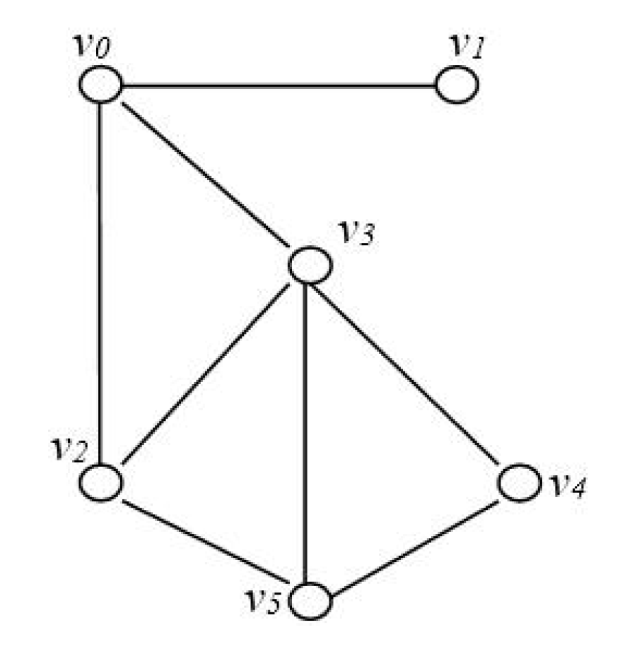
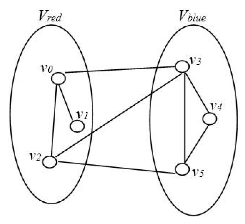
Suppose a graph G = (V, E) is given in Figure 1. Let |V| = 6, |E| = 8, and then the best solution for MLCP of graph G is shown in Figure 2, and its best value is 2.

3.2. Initial Population

The algorithm randomly generates population X consisting of p individuals. For the given graph G = (V, E), in which V is a set containing n vertices, and E is a set containing l edges, m vertices are chosen at random from V to construct set V_red (m is the initial number of the red vertices); and the remaining vertices are used to construct set V_blue, that is, |V_red| = m, V_blue = V\V_red. Sets V_red and V_blue are seen as a bipartition scheme (V_red, V_blue), which is also treated as an individual in population X. In this way, p individuals are generated at random initially, and population X is thus constructed, |X| = p.

3.3. Data Splitting Operation

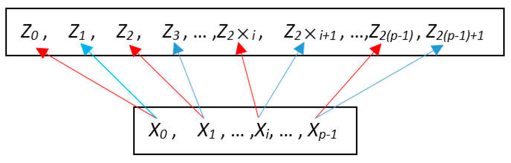
To avoid the defect of the local optima, we expand the data amount of population X, hence we get an expanded scope of data search. We use two data splitting strategies to split a bipartition scheme into two. Thus, by using the first data splitting strategy each individual X_i (0 ≤ i < p) in population X generates an individual Z_2×i, and by using the second data splitting strategy each individual X_i (0 ≤ i < p) generates an individual Z_2×i+1. By doing this, p individuals in population X are divided into 2 × p individuals, and the enlarged population Z is constructed (|X| = p, |Z| = 2 × p). Figure 3 shows the population expansion, where the red arrow indicates the effects of the first data splitting strategy and the blue arrow the effects of the second data splitting strategy.

The first data splitting strategy of bipartition scheme (V_red, V_blue) is an important part of memetic algorithm, which consists of five steps.

First step: Degree set Degree_red of all vertices in sub-graph G₁(V_red) is calculated.

Second step: Find the minimum degree vertex, v, from Degree_red. If there is more than one vertex with the same minimum degree, randomly select a vertex among them.

Third step: Degree set Degree_blue of all vertices in sub-graph G₂(V_blue) is calculated.

Fourth step: Find the minimum degree vertex, w, from Degree_blue. If there is more than one vertex with the same minimum degree, randomly select a vertex among them.

Fifth step: A new bipartition scheme (V^‘_red, V^‘_blue) is generated by exchanging the vertices v and w in sets V_red and V_blue.

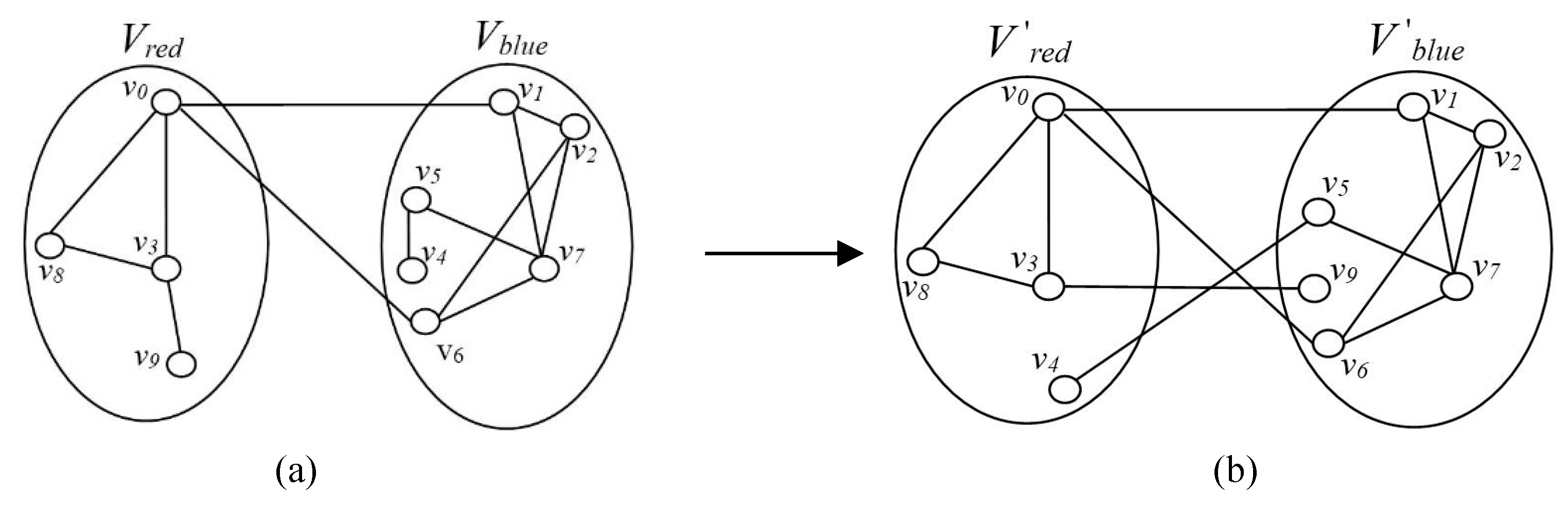
Suppose the number of red vertices is 4 in the given graph G = (V, E), V ={v₀,v₁, … ,v₉}. We obtain a bipartition scheme (V_red, V_blue), as shown in Figure 4a, in which set V_red ={v₀,v₃,v₈,v₉}, V_blue ={v₁,v₂,v₄,v₅,v₆,v₇}, where the degree of vertex v₉ in set V_red is the smallest, and that of vertex v₄ in set V_blue is the smallest. After exchanging the two vertices, a new bipartition scheme (V^‘_red, V^‘_blue) is generated. The new bipartition scheme (V^‘_red, V^‘_blue) after splitting is: V^‘_red ={v₀,v₃,v₄,v₈}, V^‘_blue ={v₁,v₂,v₅,v₆,v₇,v₉}, as shown in Figure 4b.

The second data splitting strategy is described as follows: for a given bipartition scheme (V_red, V_blue), in which |V_red| = m, V_blue = V\V_red, randomly a vertex v in set V_red is chosen, and a vertex w in set V_blue is randomly chosen. Then, vertices v and w in set V_red and set V_blue are exchanged to generate a new bipartition scheme (V″_red, V″_blue).

3.4. Search for the Individuals

Memetic algorithm needs to carry out a heuristic search for each individual in the population by an effective and improved K-OPT local search algorithm designed.

We first obtain an individual Z_j which is a (V_red, V_blue)_j, ((V_red)_j⊂V, (V_blue)_j =V\(V_red)_j, 0 ≤ j<|Z|). The local search algorithm is implemented to add as many selected vertices, acquired through our vertex adding strategy, as possible in set (V_blue)_j to set (V_red)_j, until the stop condition set by the algorithm is met. Thus, a new bipartition scheme (V_red, V_blue)’_j is constructed. Generally speaking, in (V_red, V_blue)’_j, |Er((V^‘_red)_j)|is approximately equal to |Er((V^‘_blue)_j)|. Then, the objective function value f ((V_red, V_blue)’_j) is calculated using Equation (2). If f ((V_red, V_blue)’_j) > f (s₁), the memetic algorithm accepts the constructed bipartition as the new best solution. The improved K-OPT local search algorithm is implemented by the New_K-OPT_MLCP (Algorithm 2).

Our vertex adding strategy is described as follows:

We first need to define the following three vectors as the foundation on which the vertex adding strategy is constructed.

• CC_red: The current set of red vertices in graph G.
• PAV_red: The vertex set of possible additions, i.e., each vertex is connected to at least one vertex of CC_red.

  $$PA{V}_{red}=\left\{v\right|v\in V_{blue},\exists w\in C{C}_{red},(v,w)\in E,V_{blue}=V\backslash C{C}_{red}\}.$$

  (4)
• GPAV_red: The degree set of vertices v_i$\in$PAV_red in sub-graph G^‘(PAV_red), where PAV_red ⊆ V_blue.

  $$\{\begin{array}{l}GPA{V}_{red}[i]=degre{e}_{G^{\prime }(PA{V}_{red})}(v_i)=\left|\right\{a|\forall a\in PA{V}_{red},(v_i,a)\in E\}|\\ v_i\in PA{V}_{red}\\ 0\le i\le \left|PA{V}_{red}\right|-1\end{array}.$$

  (5)

To avoid the local optima defect, the vertex adding strategy is employed in two phases: vertex addition phase (Algorithm 2, Lines 8–12) and vertex deletion phase (Algorithm 2, Lines 14–18).

In the vertex addition phase of CC_red, we obtain PAV_red from the current CC_red, then select a vertex w from PAV_red and move it from V_blue to CC_red, and finally update PAV_red. The vertex addition phase is repeatedly executed until PAV_red = $\varnothing$ or |Er(CC_red)| > |Er(V_blue)|.

In the vertex deletion phase of CC_red, we select a vertex u from CC_red, then delete the vertex u from CC_red, and add it to V_blue. Go back to the vertex addition phase again to continue the execution until the set ending conditions are met.

The approach to select vertex w is first to obtain a GPAV_red in sub-graph G’(PAV_red), then to calculate the vertex selection probability value ρ(w_i) of each vertex w_i (0 ≤ i < |PAV_red|) in PAV_red, and finally to select vertex w_i to maximize ρ(w_i). If there are more than one vertex with the maximum value of ρ(w_i), randomly select one.

$$\{\begin{array}{l}\mathrm{maxd}=\underset{w_i\in PA{V}_{red},0\le i<\left|PA{V}_{red}\right|}{\max }(degre{e}_{G^{\prime }(PA{V}_{red})}(w_i))\\ \rho (w_i)=\frac{\mathrm{maxd}+1-GPA{V}_{red}\left[\mathrm{i}\right]}{\mathrm{maxd}+1}\\ w_i\in PA{V}_{red}\\ 0\le i<\left|PA{V}_{red}\right|\end{array}.$$

(6)

A vertex w is selected according to the following criterion:

$$f_1(w)=\underset{0\le i<\left|PA{V}_{red}\right|}{\max }(\rho (w_i)).$$

(7)

We found that the larger the probability value ρ(w_i) of vertex w_i is, the smaller the degree value of vertex w_i becomes.

The approach of vertex u selection is as follows: we assume that (CC_red, V_blue)^(j) is the bipartition scheme with no possible additions. We successively take the value of i from the range of 0 – (|CC_red| $-$ 1), and then in turn execute CC_red^(j)\{u_i} as follows: delete vertex u_i from CC_red^(j) successively to generate new bipartition schemes (CC^‘_red, V^‘_blue)_i, i.e., (CC^‘_red)_i ←CC_red^(j)\{u_i}, (V^‘_blue)_i ←V_blue^(j)$\cup${u_i}, u_i$\in$CC_red, 0 ≤ i <|CC_red|, and finally obtain Ed((CC^‘_red, V^‘_blue)_i).

$$\{\begin{array}{l}Ed((C{C}_{red}^{\prime },V_{blue}^{\prime }{)}_i)=|\{(x,y)|\forall (x,y)\in E,x\in (C{C}_{red}^{\prime }{)}_i,y\in (V_{blue}^{\prime }{)}_i\left\}\right|\\ (V_{blue}^{\prime }{)}_i=V\backslash (C{C}_{red}^{\prime }{)}_i\\ 0\le i<\left|C{C}_{red}{}^{(j)}\right|\end{array}.$$

(8)

The maximum value maxdd is found from all the values of Ed, and the vertex selection probability value ρ₂(u_i) of vertex u_i can be calculated:

$$\{\begin{array}{l}\max dd=\underset{0\le i<\left|C{C}_{red}{}^{(j)}\right|}{\max }(Ed((C{C}_{red}^{\prime },V_{blue}^{\prime }{)}_i))\\ {\rho }_2(u_i)=\frac{\max dd+1-Ed({(C{C}_{red}^{\prime },V_{blue}^{\prime })}_i)}{\max dd+1}\\ u_i\in C{C}_{red}{}^{(j)}\\ 0\le i<\left|C{C}_{red}{}^{(j)}\right|\end{array}$$

(9)

A vertex u is selected according to the following criterion:

$$f_2(u)=\underset{u_i\in C{C}_{red}{}^{(j)},0\le i<\left|C{C}_{red}{}^{(j)}\right|}{\max }({\rho }_2(u_i)).$$

(10)

We found that the larger the probability value ρ₂(u_i) of vertex u_i is, the smaller the corresponding Ed ((CC^‘_red, V^‘_blue)_i) becomes. If there are more than one vertices with the maximum value of ρ₂(u_i), randomly select one.

At each generation, the variable gA stores the value of vertices number successfully added to the CC_red for now, and the variable gmaxA stores the value of vertices number successfully added to the CC_red during the previous generations. If gA > gmaxA, the incumbent CC_red has more red vertices than the previous ones found by the local search algorithm. Then, gmaxA is updated with the value of gA and the incumbent CC_red is stored to the set Abest (Algorithm 2, Line 12). In the vertex addition phase, the value of gA + 1 replaces that of gA (gA ← gA + 1) after a vertex is added. In the vertex deletion phase, the value of gA − 1 replaces that of gA (gA ← gA − 1) after a vertex is deleted.

At the completion of the inner loop statements, when gmaxA > 0, CC_red, which has the greatest number of vertices, is stored in set Abest, then the incumbent CC_red is updated with Abest. When gmaxA = 0, CC_red, which has the greatest number of vertices, is stored in set Aprev; if the execution of the inner loop does not find any new set CC_red that has more vertices, Aprev is adopted as CC_red generated by the previous execution of the inner loop and will replace the incumbent CC_red (Algorithm 2, Lines 22–28).

The algorithm’s search efficiency may be reduced because of the roundabout searching characteristics. To solve this problem, a restricting tabu table is added to the local search algorithm.

The tabu table can be presented by two-dimensional array or one-dimensional array. We adopt the one-dimensional array T, set the tabu tenure value as L, and store the iteration numbers of running the local search algorithm into the tabu table. When the algorithm runs reach iteration value c, and if (c − T[w]) < L or if (c −T[u]) < L, it means vertex w or u has been processed and the vertex should be re-selected. Otherwise, the current value c is stored in the tabu table, i.e.,T[w] ← c or T[u] ← c.

Algorithm 2 New_K-OPT_MLCP (G, Zj, T, L).

Require:

Zj: the jth individual (Vred, Vblue)j, (Vred)j⊂V, (Vblue)j = V\(Vred)j

T: tabu table

L: tabu tenure value

Output: s2, the solution found by local search algorithm

begin

1 (CCred, Vblue) ← (Vred, Vblue)j;

2 according to CCred and Vblue, PAVred and GPAVred are obtained;

3 repeat

4 Aprev ← CCred, DA ← Aprev, PL ←{v0, v1, …… vn-1}, gA ← 0, gmaxA ← 0, c ← 0;

5 repeat

6   c ← c + 1;

7   if |PAVred∩PL| > 0 and |Er(CCred)| < |Er(Vblue)| then

8   select vertex w according to f1(w), if there are multiple vertices, select a vertex w randomly;

9   if c − T[w] < L then select a non-tabu vertex w according to f1(w);

10   T[w] ← c;

11   CCred ← CCred∪{w}, Vblue ←Vblue\{w}, gA ← gA + 1, PL ← PL\{w};

12   if gA > gmaxA then gmaxA ← gA, Abest ← CCred;

13   else

14   select vertex u according to f2(u), if there are multiple vertices, select a vertex u randomly;

15   if c − T[u] < L then select a non-tabu vertex u according to f2(u);

16   T[u] ← c;

17   CCred ← CCred\{u}, Vblue ← Vblue∪{u}, gA ← gA−1, PL ← PL\{u};

18   if u∈Aprev then DA ← DA\{u};

19   end if

20   based on CCred and Vblue, PAVred and GPAVred are updated;

21  until |DA| = 0 or the cut-off time condition for CPU running is met;

22  if gmaxA > 0 then

23   CCred ← Abest;

24   Vblue ← V\CCred;

25  else

26   CCred ← Aprev;

27   Vblue ← V\CCred;

28  end if

29 until gmaxA ≤ 0 or the cut-off time condition for CPU running is met;

30 (Vred, Vblue)j ← (CCred, Vblue);

31 s2 ← (Vred, Vblue)j;

32 return s2;

end

3.5. Evolutionary Operation of Population

An evolutionary operation in the population X is needed to quickly find the best solution of MLCP. We sort the individuals Z_j (0 ≤ j < 2×p) in population Z in ascending order according to the calculated value of objective function f_* in Equation (11). Then, we replace the individuals X₀ –X_p−1 of population X with the individuals Z₀ –Z_p−1 to complete the evolutionary operation.

$$f_{*}({(V_{red},V_{blue})}_j)=|\{(a,b)|\forall (a,b)\in E,a\in {(V_{red})}_j,b\in {(V_{blue})}_j\}|,0\le j<2\times p.$$

(11)

Evolution operation of the population is represented by Evolution_population (Algorithm 3).

Algorithm 3 Evolution_population (Z, X).

Require:

Z: population, |Z| =2 × p

Output: population X

begin

1 j ← 0;

2 while j < 2 × p do

3 R[j] ← f* ((Vred, Vblue)j);

4 j ← j + 1;

5 end while

6 Individuals Z0 –Z2×p −1 of population Z are sorted in ascending order according to the value of set R;

7 (X0–Xp −1) ←(Z0–Zp −1);

8 return X;

end

3.6. Disturbance Operation

To further improve the search ability of the algorithm and find better values, we add a disturbance operation into the memetic algorithm. This disturbance operation is executed k times.

When the number of iterations is b, disturbance operation begins and randomly selects an individual (V_red, V_blue)_j (0 ≤ j < |X|) from population X, and chooses at random a vertex from set V_red and a vertex from set V_blue, then the two vertices are exchanged to generate a new (V_red, V_blue)’. Then, employ the New_K-OPT_MLCP algorithm to search in (V_red, V_blue)’; if a better solution of MLCP is found, the memetic algorithm will accept it.

The disturbance operation is represented by Disturbance_operation (Algorithm 4).

Algorithm 4 Disturbance_operation(X, b, k, d1, d2, Wbest).

Require:

X: set that stores the population

b, k: control parameters of disturbance operation

d1, d2: control variables of disturbance operation

Wbest: variable that stores the value of the objective function f(st), in which st is the current best solution of MLCP

Output: s1, a better solution found by the local search algorithm

f(s1), the value of the objective function

d1, d2, values of the control variables

begin

1 d1 ← d1 + 1;

2 if d1 = b then

3 d2 ← d2 + 1;

4 if d2 ≤ k then

5   if d2 = 1 then

6   randomly choose Xj from X and start disturbance to generate a new X‘j;

7   W ← New_K-OPT_MLCP (G, X‘j, T, L);

8   if f (W) > Wbest then s1 ← W, Wbest ← f (W);

9   t ← X‘j ;

10  else

11   start disturbance t to generate a new t‘ ;

12   W ← New_K-OPT_MLCP (G, t‘, T, L);

13   if f (W) > Wbest then s1 ← W, Wbest ← f (W);

14   t ← t‘;

15  end if

16  d1 ← d1 − 1

17  else

18  d1 ← 0, d2 ← 0;

19  end if

20 end if

21 return s1, Wbest, d1, d2;

end

In Memetic_D_O_MLCP algorithm, setting the value of b and k will determine the disturbance operation’s starting condition and the number of times of its execution. In Disturbance_operation algorithm, Lines 1, 3, 16, and 18 store the modified values of variables d1 and d2, which are the threshold values needed to start off a new disturbance operation.

4. Simulated Annealing Algorithm

Simulated annealing algorithm, a classical heuristic algorithm to solve combinatorial optimization problems, starts off from a higher initial temperature. With the decreasing of temperature parameters, the algorithm can randomly find the global best solution of problems instead of the local optima by combining the perturbations triggered by the probabilities.

For a given graph G, simulated annealing algorithm finds a coloring bipartition scheme (V_red, V_blue) of V which maximizes min{|Er(V_red)|, |Er(V_blue)|}. With parameters T₀ (initial temperature value), α (cooling coefficient) and T_end (the end temperature value), first, the algorithm divides the vertex set V into two sets, i.e., V_red and V_blue (V_red = $\varnothing$, V_blue = V) and the initial value of the best solution of MLCP C_best is set to 0. Next, a vertex is randomly selected in V_blue and moved from V_blue to V_red; here, |V_red| = 1, V_blue = V\V_red. Then, the algorithm repeats a series of generations to explore the search space defined by the set of all 2-colorings. At each generation, a vertex is randomly selected in V_blue and moved from V_blue to V_red. The additions will take place in the following three forms:

When 2 > |V_red| and 2 ≤ |V_blue|, a vertex is randomly selected in V_blue and moved from V_blue to V_red to generate a new coloring bipartition scheme (V^‘_red, V^‘_blue) and the new status is accepted.

When 2 > |V_blue| and 2 ≤ |V_red|, a vertex is randomly selected in V_red and moved from V_red to V_blue to generate a new coloring bipartition scheme (V^‘_red, V^‘_blue) and accepted as the new status.

When 2 ≤ |V_red| and 2 ≤ |V_blue|, a vertex is randomly selected from V_red and one randomly from V_blue, then the two vertices are exchanged to generate a new coloring bipartition scheme (V^‘_red, V^‘_blue), only when R₁((V^‘_red, V^‘_blue)) ≥ R₁((V_red, V_blue)), the scheme is accepted as a new status. Otherwise, the probability will decide whether to accept it as a new status or not.

Once the new status is accepted, if C_best < R₁ ((V^‘_red, V^‘_blue)), then the bipartition scheme (V^‘_red, V^‘_blue) is accepted as the best solution of MLCP.

At the end of each generation, the temperature T cools down until T ≤T_end according to T = T × α, where α$\in$(0,1). The algorithm runs iteratively as per the above steps until the stop condition is met.

The best solution found by the algorithm is R_b((V_red, V_blue)), i.e.,

$$\{\begin{array}{l}{R}_1((V_{red},V_{blue}{)}_j)=\min \{|Er((V_{red}{)}_j)|,|Er((V_{blue}{)}_j)|\}\\ R_b((V_{red},V_{blue}))=\underset{0\le j<t}{\max }\{R_1((V_{red},V_{blue}{)}_j)\}\end{array}.$$

(12)

Here, t is the number of all solutions that can be found by the simulated annealing algorithm in graph G, and (V_red, V_blue)_j is the jth solution of MLCP.

The simulated annealing algorithm is represented by SA (Algorithm 5).

Algorithm 5 SA(G, Vred, Vblue, T0, α, Tend).

Require: G: G = (V, E), |V| = n, |E| = l

Vred: a set of red vertices in graph G

Vblue: a set of blue vertices in graph G

T0: initial temperature value

α: cooling coefficient

Tend: end temperature value

Output: s3, the best solution found by SA algorithm

R1(s3), value of the objective function

begin

1 Cbest ← 0;

2 repeat

3 T ← T0;

4 initialize Vred and Vblue, randomly select a vertex in Vblue and moved from Vblue to Vred;

5 while T > Tend do

6   if 2 > |Vred| and 2 ≤ |Vblue| then

7   a vertex is randomly selected in Vblue and moved from Vblue to Vred to generate a new bipartition scheme (V‘red, V‘blue);

8  (Vred, Vblue) ← (V‘red, V‘blue);

9  if Cbest < R1((V‘red, V‘blue)) then Cbest ←R1((V‘red, V‘blue)), s3 ← (V‘red, V‘blue);

10 else if 2 > |Vblue| and 2 ≤ |Vred| then

11   a vertex is randomly selected in Vred and moved from Vred to Vblue to generate a new bipartition scheme (V‘red, V‘blue);

12   (Vred, Vblue) ← (V‘red, V‘blue);

13   if Cbest < R1 ((V‘red, V‘blue)) then Cbest ← R1 ((V‘red, V‘blue)), s3 ← (V‘red, V‘blue);

14 else if 2 ≤ |Vred| and 2 ≤ |Vblue| then

15   according to (Vred, Vblue), a vertex is randomly selected from Vred and a vertex randomly selected from Vblue;

16   the two vertices are exchanged to generate a new bipartition scheme (V‘red, V‘blue);

17   if R1 ((Vred, Vblue)) ≤ R1((V‘red, V‘blue)) then

18   (Vred, Vblue) ← (V‘red, V‘blue);

19   if Cbest < R1((V‘red, V‘blue)) then Cbest ← R1((V‘red, V‘blue)), s3 ← (V‘red, V‘blue);

20   else if random number in (0, 1) < $e^{\frac{R_1((V_{red}^{’},V_{blue}^{’}))-R_1((V_{red},V_{blue}))}{T}}$ then

21   (Vred, Vblue) ← (V‘red, V‘ blue);

22  end if

23 end if

24 T ← T × α;

25  end while

26 until stop condition is met;

27 return s3, Cbest;  /*Cbest is the value of the objective function R1(s3) */

end

5. Greedy Algorithm

Greedy algorithm aims at making the optimal choice at each stage with the hope of finding a global best solution. For a given graph G, greedy algorithm finds a coloring bipartition scheme (V_red, V_blue) of V which maximizes min{|Er(V_red)|, |Er(V_blue)|}.

When a graph G = (V, E) is given, the algorithm divides vertex set V into two sets, i.e., V_red and V_blue (V_red = $\varnothing$, V_blue = V), and the initial value of the best solution of MLCP C_best is set to 0. Next, a vertex is randomly selected in V_blue and moved from V_blue to V_red, here |V_red | = 1, V_blue = V\V_red. Then, the algorithm repeats a series of generations to explore the search space defined by the set of all 2-colorings. At each generation, based on sub-graph G^‘(V_blue), choose a vertex w of the minimum degree (w$\in$V_blue); if there are more than one vertex with the same minimum degree, randomly select a vertex among them. Then, add the vertex from V_blue to V_red, that is: V_red ← V_red$\cup${w}, V_blue ← V_blue\{w}, thus a new bipartition scheme (V^‘_red, V^‘_blue) is generated, and, when R₂((V^‘_red,V^‘_blue)) > C_best, the scheme is accepted as the best solution. The generation will be repeated until |Er(V_red)| > |Er(V_blue)|.

The algorithm runs iteratively as per the above steps until the stop condition is met.

The best solution found by the algorithm is R_g((V_red,V_blue)), i.e.,

$$\{\begin{array}{l}{R}_2((V_{red},V_{blue}{)}_j)=\min \{|Er((V_{red}{)}_j)|,|Er((V_{blue}{)}_j)|\}\\ R_g((V_{red},V_{blue}))=\underset{0\le j<t}{\max }\{R_2((V_{red},V_{blue}{)}_j)\}\end{array}.$$

(13)

Here, t is the number of all solutions that can be found by the greedy algorithm in graph G, and (V_red, V_blue)_j is the jth solution of MLCP.

The greedy algorithm is represented by Greedy (Algorithm 6).

Algorithm 6 Greedy (G, Vred, Vblue).

Require: G: G = (V, E), |V| = n, |E| = l

Vred: a set of red vertices in graph G

Vblue: a set of blue vertices in graph G

Output: s4, the best solution found by greedy algorithm

R2(s4), value of the objective function

begin

1 Cbest ←0;

2 repeat

3 Vred ←Ø, Vblue ← V;

4 randomly select a vertex in Vblue and moved from Vblue to Vred;

5 repeat

6   (V’red, V’blue) ← (Vred, Vblue);

7   if R2((V’red, V’blue)) > Cbest then s4 ← (V’red, V’blue), Cbest ← R2 ((V’red, V’blue));

8    select a vertex w with the minimum degree from sub-graph G‘(Vblue), if there are multiple vertices, select a vertex w randomly;

9    Vred ← Vred ∪ {w}, Vblue ← Vblue\{w};

10  until |Er(Vred)| > |Er(Vblue)|;

11 until stop condition is met;

12 return s4, Cbest;  /* Cbest is the value of the objective function R2 (s4) */

end

6. Experimental Results

All algorithms were programmed in C++, and run on a PC with Intel Pentium(R) G630 processor 2.70 GHz and 4 GB memory under Windows 7 (64 bits), and the test graphs adopted were the benchmark DIMACS proposed in [5]. We compared the search results by using memetic algorithm, simulated annealing algorithm, and greedy algorithm. Then, the results of memetic algorithm were compared with those obtained from using artificial bee colony algorithm [4], tabu search algorithm [5] and variable neighborhood search algorithm [5].

The first group of experiments was performed to adjust the key parameters and analyze their influence on Memetic_D_O_MLCP. As is known to all, the most important parameters in Memetic_D_O_MLCP implementations are the values of p and L, which determine the number of the individuals of the population and the tabu tenure value during the search process. To find the most suitable values of p and L for Memetic_D_O_MLCP approach to MLCP, we performed experiments with different values of p and L. Memetic_D_O_MLCP was run 10 times for each benchmark instance, and each test lasted 30 min.

The results of experiments are summarized in

Table 1. Experiments with parameters p and L.

Inst	m	p = 4						p = 12						p = 20
		L = 10		L = 60		L = 90		L = 10		L = 60		L = 90		L = 10		L = 60		L = 90
		Best	Avg	Best	Avg	Best	Avg	Best	Avg	Best	Avg	Best	Avg	Best	Avg	Best	Avg	Best	Avg
fpsol2.i.1.col	|V|/5	3035	2844	3033	2857	3582	2928	3015	2840	3002	2845	3029	2837	3071	2929	2942	2727	2998	2843
fpsol2.i.2.col	|V|/5	2120	1965	2375	1953	2183	1860	2272	1972	2176	1944	2450	1969	2324	2016	2169	1932	2310	2038
fpsol2.i.3.col	|V|/5	2141	1930	2331	1931	2266	2048	2333	1960	2330	1930	2115	1900	1981	1817	2397	1986	2281	1951
DSJC125.1.col	|V|/5	255	252	254	252	254	251	254	252	255	252	255	252	254	252	255	253	254	252
DSJC125.5.col	|V|/5	1081	1072	1082	1067	1088	1078	1084	1076	1087	1080	1089	1080	1084	1078	1087	1072	1084	1074
queen15_15.col	|V|/5	1716	1699	1721	1678	1721	1694	1693	1650	1705	1692	1716	1681	1659	1632	1704	1638	1674	1641
queen16_16.col	|V|/5	2090	2050	2087	2049	2087	2055	2040	1976	2062	1994	2098	2026	2036	1990	2032	1995	2040	1996
mulsol.i.4.col	|V|/5	1704	1694	1704	1698	1704	1694	1701	1695	1704	1696	1704	1698	1700	1697	1704	1697	1704	1694

, organized as follows: in the first column, Inst the benchmark instance name is given, containing the vertices set V; and, in the second column, m is the initial number of red vertices in the benchmark graph. For each p$\in${4, 12, 20} and L$\in${10, 60, 90}, column Best contains the best values of MLCP solution found by the algorithm, while column Avg represents the average values of MLCP solution found by the algorithm. For each instance, the best values of Best and Avg are shown in italics. The analysis of the obtained results shows that values of p and L influence the solution quality. For example, the number of best values of Best is 5 for combination p = 12 and L = 90; Best 3 for p = 4, L = 90 and p = 20, L = 60; Best 2 for p = 4 and L = 10, p = 4 and L = 60, p = 12 and L = 60; Best 1 for p = 20 and L = 90; Best 0 for p = 12 and L = 10, p = 20 and L = 10. Meanwhile, the number of best values of Avg is 2 for combinations p = 12 and L = 90, p = 4 and L = 90; Avg 1 for p = 4 and L = 10, p = 4 and L = 60, p = 12 and L = 60, p = 20 and L = 10, p = 20 and L = 60, p = 20 and L = 90.

In Table 1, one observes that, for combination p = 12 and L = 90, the number of instances where the Memetic_D_O_MLCP achieved the best value for Best and Avg is 5 and 2, respectively. For all other combinations, these numbers are the biggest. Therefore, we used the combination in all other experiments.

The second groups of tests compared the search results of Memetic_D_O_MLCP, SA algorithm and Greedy algorithm, each having been run 20 times for each benchmark instance with the cut-off time of 30 min. In simulated annealing algorithm, the initial temperature T₀ is set at 1000, the cooling coefficient α at 0.9999 and the end temperature T_end at 0.0001. The results of experiments are summarized in

Table 2. Test results of the Memetic_D_O_MLCP, SA, and Greedy on benchmark instances.

Inst	|V|	|E|	Memetic_D_O_MLCP			SA		Greedy
			m	Best	Avg	Best	Avg	Best	Avg
anna.col	138	986	|V|/5	200	198	160	154	131	131
david.col	87	812	|V|/5	158	157	133	130	140	140
DSJC125.1.col	125	736	|V|/5	255	252	222	217	240	238
DSJC125.5.col	125	3891	|V|/5	1091	1083	1025	1021	1075	1067
DSJC125.9.col	125	6961	|V|/5	1798	1789	1761	1756	1776	1772
fpsol2.i.1.col	496	11654	|V|/5	3091	2896	3016	2982	2510	2502
fpsol2.i.2.col	451	8691	|V|/5	2290	2046	2267	2242	1707	1703
fpsol2.i.3.col	425	8688	|V|/5	2387	1996	2291	2247	1664	1664
games120.col	120	1276	|V|/5	288	281	215	209	284	284
homer.col	561	3258	10	662	655	450	441	492	489
huck.col	74	602	|V|/5	130	129	111	109	113	113
inithx.i.1.col	864	18707	10	6644	6153	4861	4773	6167	6050
inithx.i.2.col	645	13979	10	5622	5104	3641	3597	3571	3481
inithx.i.3.col	621	13969	10	5589	4756	3643	3593	3131	3111
jean.col	80	508	|V|/5	111	110	98	95	106	106
latin_square_10.col	900	307350	10	85161	85072	77006	75770	85185	85185
le450_5a.col	450	5714	10	1824	1801	1516	1495	1834	1827
le450_5b.col	450	5734	10	1820	1801	1512	1498	1843	1831
le450_5c.col	450	9803	10	2985	2951	2541	2530	3014	2995
le450_5d.col	450	9757	10	2943	2913	2542	2519	2972	2958
le450_15b.col	450	8169	10	2395	2355	2138	2120	2409	2398
le450_15c.col	450	16680	10	4530	4476	4294	4267	4560	4539
le450_15d.col	450	16750	10	4586	4542	4320	4289	4626	4609
le450_25a.col	450	8260	10	2467	2434	2183	2148	2466	2454
le450_25b.col	450	8263	10	2664	2606	2172	2149	2682	2658
le450_25c.col	450	17343	10	4711	4652	4457	4438	4728	4714
le450_25d.col	450	17425	10	4872	4807	4470	4449	4883	4875
miles250.col	128	774	|V|/5	185	184	145	137	183	183
miles500.col	128	2340	|V|/5	522	522	393	381	518	518
miles750.col	128	4226	|V|/5	870	870	673	638	849	849
miles1000.col	128	6432	|V|/5	1183	1180	954	921	1156	1156
miles1500.col	128	10396	|V|/5	1645	1616	1461	1421	1485	1484
mulsol.i.1.col	197	3925	|V|/5	1697	1690	1193	1152	1624	1624
mulsol.i.2.col	188	3885	|V|/5	1685	1682	1153	1117	1202	1189
mulsol.i.3.col	184	3916	|V|/5	1695	1692	1174	1131	1211	1174
mulsol.i.4.col	185	2946	|V|/5	1704	1701	1172	1134	1218	1195
mulsol.i.5.col	186	3973	|V|/5	1714	1713	1189	1144	1216	1210
myciel3.col	11	20	|V|/5	5	5	5	5	5	5
myciel4.col	23	71	|V|/5	21	21	21	21	21	21
myciel6.col	95	755	|V|/5	233	231	215	212	194	193
myciel7.col	191	2360	|V|/5	723	717	643	634	574	574
queen5_5.col	25	320	|V|/5	46	46	46	46	46	46
queen6_6.col	36	580	|V|/5	91	91	91	88	91	91
queen7_7.col	49	952	|V|/5	148	147	145	141	148	148
queen8_8.col	64	1456	|V|/5	236	232	219	214	236	228
queen8_12.col	96	2736	|V|/5	458	453	400	391	458	458
queen9_9.col	81	2112	|V|/5	340	336	308	304	340	334
queen10_10.col	100	2940	|V|/5	485	479	419	415	468	466
queen11_11.col	121	3960	|V|/5	644	643	563	556	633	633
queen12_12.col	144	5192	|V|/5	866	853	725	717	833	833
queen13_13.col	169	6656	|V|/5	1097	1093	918	909	1067	1067
queen14_14.col	196	8372	|V|/5	1407	1385	1148	1131	1346	1345
queen15_15.col	225	10360	|V|/5	1721	1706	1402	1376	1676	1675
queen16_16.col	256	12640	|V|/5	2107	2075	1668	1652	2051	2048
school1.col	385	19095	10	6633	6553	4951	4886	6644	6644
school1_nsh.col	352	14612	10	5545	5450	3838	3780	5548	5548
zeroin.i.1.col	211	4100	10	1210	1198	1113	1095	924	923
zeroin.i.2.col	211	3541	10	1135	1126	975	959	803	800
zeroin.i.3.col	206	3540	10	1134	1126	981	964	800	799

, organized as follows: in the second column, |V| is the number of vertices; and, in the third column, |E| is the number of edges. For each instance the best values of Best are shown in italics. Among 59 instances, the search results of Memetic_D_O_MLCP, SA algorithm and Greedy algorithm were the same in the instances myciel3.col, myciel4.col, queen5_5.col and queen6_6.col. Memetic_D_O_MLCP and Greedy algorithm could find equivalent best value of four instances (i.e., queen7_7.col, queen8_8.col, queen8_12.col, and queen9_9.col). In the remaining 51 instances, Memetic_D_O_MLCP could find the best results of 38 instances (accounting for 75%), and Greedy algorithm could find the best results of 13 instances (accounting for 25%). The experiments showed that Memetic_D_O_MLCP could find more instances of best values.

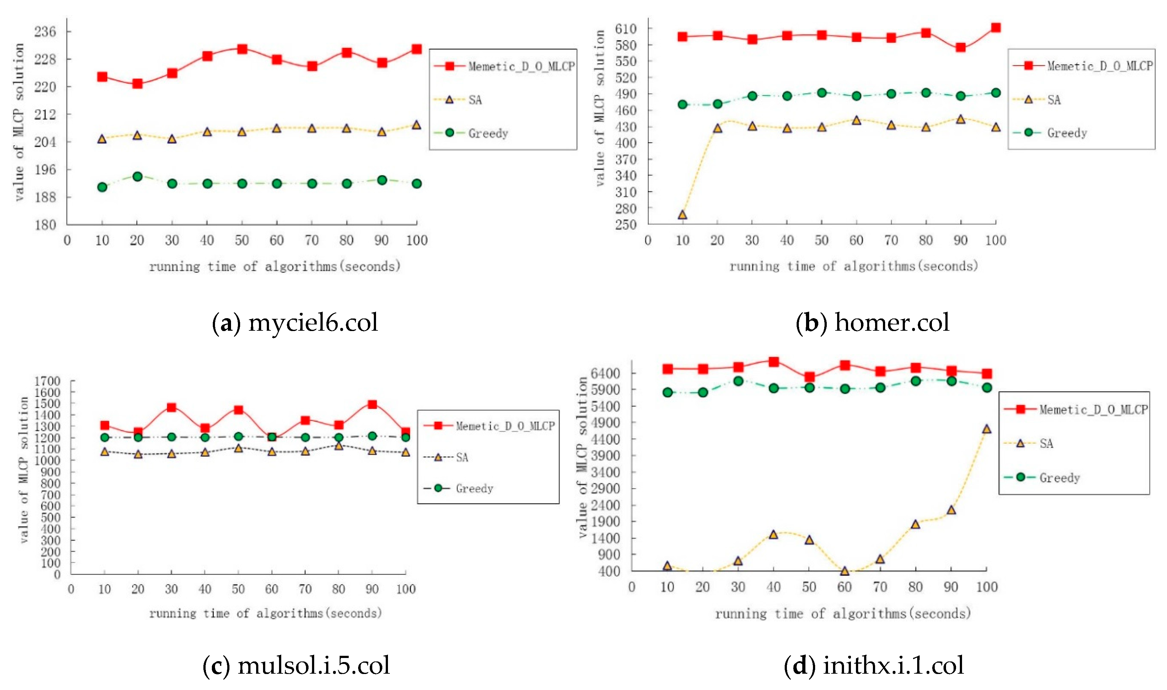
The third group of tests aimed at comparing the search results after each algorithm was run on four benchmark instances, namely myciel6.col, homer.col, mulsol.i.5.col and inithx.i.1.col, for the first one 100 s. The results that algorithms found were collected at an interval of 10 s. The running time was regarded as the X coordinate on the axis and the value of MLCP solution as the Y coordinate.

Figure 5 illustrates that Memetic_D_O_MLCP can find the best result at each time node.

The fourth group of tests compared the time each algorithm took to find the best results, each being run 20 times for 32 instances with the cut-off time of 30 min.

The results are summarized in

Table 3. Running time of the Memetic_D_O_MLCP, SA and Greedy on benchmark instances.

Inst	Memetic_D_O_MLCP				SA			Greedy
	m	Best	Avg	Time(min)	Best	Avg	Time(min)	Best	Avg	Time(min)
anna.col	|V|/5	200	199	5.30	159	150	17.29	131	131	0.09
david.col	|V|/5	158	157	0.47	140	130	21.97	140	140	0.02
DSJC125.1.col	|V|/5	254	252	27.92	220	214	29.76	239	237	19.24
DSJC125.5.col	|V|/5	1086	1078	22.82	1026	1012	28.20	1075	1067	14.07
DSJC125.9.col	|V|/5	1797	1785	18.86	1757	1752	14.04	1782	1773	17.81
fpsol2.i.1.col	|V|/5	3073	2871	23.52	2984	2966	13.42	2510	2504	4.78
fpsol2.i.2.col	|V|/5	2274	1882	17.20	2250	2226	25.58	1707	1706	22.30
games120.col	|V|/5	288	280	1.05	216	205	29.74	284	284	0.05
huck.col	|V|/5	130	129	0.03	113	109	6.86	113	113	0.09
miles250.col	|V|/5	185	184	5.92	140	134	29.67	183	183	4.05
miles500.col	|V|/5	522	522	1.11	389	375	25.71	518	518	< 0.01
miles750.col	|V|/5	870	870	1.72	644	618	17.17	849	849	0.07
miles1000.col	|V|/5	1186	1178	18.53	938	892	24.83	1156	1156	0.22
miles1500.col	|V|/5	1619	1613	27.56	1453	1411	15.90	1485	1485	2.36
mulsol.i.1.col	|V|/5	1695	1689	20.94	1164	1089	28.06	1624	1624	0.29
mulsol.i.2.col	|V|/5	1685	1680	26.63	1157	1065	22.97	1202	1188	8.10
mulsol.i.3.col	|V|/5	1693	1687	22.76	1147	1112	23.56	1209	1183	25.14
mulsol.i.4.col	|V|/5	1704	1694	25.22	1139	1091	29.25	1218	1186	28.08
mulsol.i.5.col	|V|/5	1714	1705	23.77	1165	1093	20.23	1214	1207	28.68
jean.col	|V|/5	111	110	0.13	97	93	18.93	106	106	0.02
myciel6.col	|V|/5	232	231	20.01	213	211	19.19	194	192	26.07
myciel7.col	|V|/5	719	710	18.73	631	624	27.23	574	574	3.68
queen10_10.col	|V|/5	485	478	1.42	418	410	10.08	468	466	21.61
queen11_11.col	|V|/5	644	643	2.56	554	539	21.94	640	633	12.95
queen12_12.col	|V|/5	866	853	5.32	721	703	22.64	833	833	0.07
queen13_13.col	|V|/5	1097	1093	25.21	907	884	21.66	1067	1067	2.98
queen15_15.col	|V|/5	1697	1675	21.65	1377	1357	29.27	1676	1675	26.07
inithx.i.1.col	10	6622	5982	23.36	4774	4696	11.55	6169	6044	1.45
inithx.i.3.col	10	5362	4123	22.89	3616	3569	9.58	3151	3117	22.93
zeroin.i.1.col	10	1207	1189	12.76	1111	1083	19.77	924	923	5.78
zeroin.i.2.col	10	1131	1124	18.46	967	939	21.43	802	799	26.64
zeroin.i.3.col	10	1131	1125	28.96	959	937	28.32	800	798	10.53

. Compared with SA algorithm and Greedy algorithm, it took less time for Memetic_D_O_MLCP to find the best results for the 11 instances (shown in italics). Accounting for 34% in the total, these 11 instances were: fpsol2.i.2.col, huck.col, mulsol.i.3.col, mulsol.i.4.col, mulsol.i.5.col, myciel6.col, queen10_10.col, queen11_11.col, queen15_15.col, inithx.i.3.col, and zeroin.i.2.col. For six instances, namely david.col, DSJC125.9.col, games120.col, miles250.col, miles750.col, and jean.col, which accounted for 19% in the total, the time spent by Memetic_D_O_MLCP and Greedy algorithm showed little difference. Additionally, the former found better results than the latter. For the remaining 15 instances, although the time taken by Memetic_D_O_MLCP was longer than that by Greedy algorithm, as it consumed more time for executing the operations of data splitting, searching, evolution and disturbance, the results found by the former were better than those by the latter. Of all 32 instances, comparing with Memetic_D_O_MLCP, SA algorithm spent more time to find the best results; besides, the Best SA algorithm results were inferior.

The comparison between Memetic_D_O_MLCP and artificial bee colony (ABC) algorithm [4] is summarized in

Table 4. Comparison results on Memetic_D_O_MLCP and ABC.

Inst	Memetic_D_O_MLCP		ABC
	m	Best	Best
DSJC125.1.col	|V|/5	255	209
DSJC125.5.col	|V|/5	1091	1005
DSJC125.9.col	|V|/5	1798	1746
fpsol2.i.1.col	|V|/5	3091	2956
fpsol2.i.2.col	|V|/5	2290	2231
fpsol2.i.3.col	|V|/5	2387	2207
inithx.i.1.col	10	6644	1295
inithx.i.2.col	10	5622	3574
inithx.i.3.col	10	5589	3548
myciel3.col	|V|/5	5	5
myciel4.col	|V|/5	21	21
myciel5.col	|V|/5	73	68
myciel6.col	|V|/5	233	207
myciel7.col	|V|/5	723	621
le450_5a.col	10	1824	1475
le450_5b.col	10	1820	1490
le450_5c.col	10	2985	2505
le450_5d.col	10	2943	2493
le450_15b.col	10	2395	2110
le450_15c.col	10	4530	4217
le450_15d.col	10	4586	4227

. For each instance, the best values of Best are shown in italics. Of all 21 instances proposed in [4], except that the search results of instances myciel3.col and myciel4.col were equivalent to that of artificial bee colony algorithm, Memetic_D_O_MLCP found better results (accounting for 90%) and improved the best-known result of instance myciel5.col.

Furthermore, we compared the search results from Memetic_D_O_MLCP, tabu search (Tabu) algorithm [5] and variable neighborhood search (VNS) algorithm [5]; the results are shown in

Table 5. Comparison results on Memetic_D_O_MLCP, Tabu and VNS.

Inst	Memetic_D_O_MLCP			Tabu		VNS
	m	Best	Avg	Best	Avg	Best	Avg
anna.col	|V|/5	200	198	195	182	218	189
david.col	|V|/5	158	157	153	142	164	152
DSJC125.1.col	|V|/5	255	252	248	238	227	215
DSJC125.5.col	|V|/5	1091	1083	1078	1073	1047	1033
DSJC125.9.col	|V|/5	1798	1789	1794	1787	1793	1785
games120.col	|V|/5	288	281	282	269	192	181
homer.col	10	662	655	651	625	603	541
huck.col	|V|/5	130	129	130	126	123	110
inithx.i.1.col	10	6644	6153	7412	6272	6215	5838
inithx.i.2.col	10	5622	5104	5956	5831	4771	4478
inithx.i.3.col	10	5589	4756	5943	5818	4804	4464
jean.col	|V|/5	111	110	110	104	110	95
latin_square_10.col	10	85161	85072	76925	76925	77031	76956
le450_5a.col	10	1824	1801	1977	1923	1545	1520
le450_5b.col	10	1820	1801	1969	1923	1550	1522
le450_5c.col	10	2985	2951	3154	3124	2578	2553
le450_5d.col	10	2943	2913	3140	3108	2583	2546
le450_15b.col	10	2395	2355	2795	2719	2338	2268
le450_25b.col	10	2664	2606	2903	2863	2382	2337
le450_25d.col	10	4872	4807	5420	5376	4844	4747
miles250.col	|V|/5	185	184	183	172	134	126
miles500.col	|V|/5	522	522	502	483	402	367
miles750.col	|V|/5	870	870	836	833	708	648
miles1000.col	|V|/5	1183	1180	1114	1108	1035	963
miles1500.col	|V|/5	1645	1616	1517	1513	1565	1490
mulsol.i.1.col	|V|/5	1697	1690	1649	1649	1313	1240
mulsol.i.2.col	|V|/5	1685	1682	1685	1668	1319	1211
mulsol.i.3.col	|V|/5	1695	1692	1695	1669	1260	1217
mulsol.i.4.col	|V|/5	1704	1701	1704	1693	1276	1214
mulsol.i.5.col	|V|/5	1714	1713	1697	1686	1296	1233
myciel3.col	|V|/5	5	5	5	5	7	7
myciel4.col	|V|/5	21	21	21	20	25	24
myciel6.col	|V|/5	233	231	231	223	247	237
myciel7.col	|V|/5	723	717	714	701	737	711
queen5_5.col	|V|/5	46	46	46	45	50	48
queen6_6.col	|V|/5	91	91	91	90	86	82
queen7_7.col	|V|/5	148	147	148	145	142	136
queen8_8.col	|V|/5	236	232	236	233	208	201
queen8_12.col	|V|/5	458	453	458	457	380	369
queen9_9.col	|V|/5	340	336	336	332	306	293
queen10_10.col	|V|/5	485	479	485	483	403	394
queen11_11.col	|V|/5	644	643	650	637	546	536
queen12_12.col	|V|/5	866	853	866	858	703	689
queen13_13.col	|V|/5	1097	1093	1106	1066	910	887
queen14_14.col	|V|/5	1407	1385	1407	1403	1127	1101
queen15_15.col	|V|/5	1721	1707	1722	1703	1388	1366
queen16_16.col	|V|/5	2107	2075	2136	2125	1682	1650
school1.col	10	6633	6553	6975	6752	5628	5398
school1_nsh.col	10	5545	5450	5721	5622	4169	4066
zeroin.i.1.col	10	1210	1198	1185	1166	1454	1358
zeroin.i.2.col	10	1135	1126	1105	1079	1294	1201
zeroin.i.3.col	10	1134	1126	1107	1082	1221	1158

(the algorithms in the literature were run 20 times, each lasting 30 min for each benchmark instance). Memetic_D_O_MLCP could find the best results of 26 instances (shown in italics), in which the best results of 11 instances equaled those found by Tabu algorithm. Hence, Memetic_D_O_MLCP could improve the best-known results of the remaining 15 instances. Besides, of the 53 instances in Table 5, the best results of 22 instances found by Memetic_D_O_MLCP were better than those by Tabu algorithm, and the best results of 42 instances found by Memetic_D_O_MLCP were better than that of VNS algorithm.

7. Conclusions

In this paper, we propose a memetic algorithm (Memetic_D_O_MLCP) to deal with the minimum load coloring problem. The algorithm employs an improved K-OPT local search procedure with a combination of data splitting operation, disturbance operation and a population evolutionary operation to assure the quality of the search results and intensify the searching ability.

We assessed the performance of our algorithm on 59 well-known graphs from the benchmark DIMACS competitions. The algorithm could find the best results of 46 graphs. Compared with simulated annealing algorithm and greedy algorithm, which cover the best results for the tested instances, our algorithm was more competent.

In addition, we investigated the artificial bee colony algorithm, variable neighborhood search algorithm and tabu search algorithm proposed in the literature. We carried out comparative experiments between our algorithm and artificial bee colony algorithm using 21 benchmark graphs, and the experiments showed that the algorithm’s best results of 19 benchmark graphs were better than those of artificial bee colony algorithm, and the best-known result of one benchmark graph was improved by our algorithm. More experiments were conducted to compare our algorithm with tabu search algorithm and variable neighborhood search algorithm, and proved that the best-known results of 15 benchmark graphs were improved by our algorithm.

Finally, we showed that the proposed Memetic_D_O_MLCP approach significantly improved the classical heuristic search approach for the minimum load coloring problem.