Approximation-Free Output-Feedback Non-Backstepping Controller for Uncertain SISO Nonautonomous Nonlinear Pure-Feedback Systems

Abstract

A novel differentiator-based approximation-free output-feedback controller for uncertain nonautonomous nonlinear pure-feedback systems is proposed. Using high-order sliding mode observer, which is a finite-time exact differentiator, the time-derivatives of the signal generated using tracking error and filtered input are directly estimated. As a result, the proposed non-backstepping control law and stability analysis are drastically simple. The tracking error vector is guaranteed to be exponentially stable in finite time regardless of the nonautonomous property in the considered system. It does not require neural networks or fuzzy logic systems, which are typically adopted to capture unstructured uncertainties intrinsic in the controlled system. As far as the authors know, there are no research results on the output-feedback controller for the uncertain nonautonomous pure-feedback nonlinear systems. The results of the simulation show clearly the performance and compactness of the control scheme proposed.

1. Introduction

Designing a controller for nonlinear systems containing unstructured uncertainties has been considerably advanced and performed in recent years. Conventionally, many adaptive controllers using universal approximators (UAs) such as neural networks (NNs) or fuzzy logic systems (FLSs) have been proposed (refer to [1,2,3,4,5,6,7,8,9,10,11,12] and references therein). More recently, controllers for nonlinear pure-feedback systems that contain unstructured uncertainties and unmatched disturbances have been actively proposed. Adaptive backstepping with UAs or dynamic surface control (DSC) algorithm is typically adopted to induce control laws that deal with unstructured uncertainties and unmatched disturbances [10,11,12,13,14,15,16,17,18,19,20,21,22,23,24]. The pure-feedback nonlinear systems are more general than strict-feedback systems [8,25,26,27,28] because they have the nonaffine appearance of the states which are chosen as virtual controls in each intermediate design steps. As a result, it is more challenging and difficult to construct the control law for this class of systems. Previously proposed adaptive controllers are typically combining UAs with backstepping or DSC. In these control algorithms, unstructured uncertainties in the system are estimated by NNs or FLSs. The outputs of the approximators are used by the controller to compensate or cancel the effect of the unmatched or unstructured uncertainties. The conventional adaptive DSC or backstepping based controllers that adopt NNs or FLSs have the following severe drawbacks. The complexity of the control law grows significantly as the dynamic order of the controlled system increases. To evade this problem, in the DSC-based controllers, the time-derivatives of virtual controls are replaced by some filtered values of them. However, even in the DSC-based controllers, the shortcoming that many UAs are required to build virtual control in every design steps still exists. These approximators are usually trained online to cope with respective uncertainties that appear in every intermediate design step. Using too many UAs results in a significant increase in the complexity of control law. Computational burden is another crucial problem since the parameters in the approximators are to be updated simultaneously in real time.

In this paper, a new output-feedback differentiator-based controller for SISO uncertain nonautonomous pure-feedback nonlinear systems is proposed using high-order sliding mode (HOSM) observer [29,30], which is a finite-time exact differentiator. As far as the authors know, there are no research results on the output-feedback controller for the considered nonautonomous pure-feedback nonlinear systems. Inspired by [8,10,22], the original system is transformed into a Brunovsky form with respect to newly defined states which are the time-derivatives of the system output. The key idea of the proposed controller is that it utilizes HOSM observer to estimate the time-derivatives of a signal that is generated using the tracking error and filtered control input. The merits of the controller proposed are described as follows.

(i)

The powerful feature of the HOSM differentiator is used by the controller to cope with uncertainties in the controlled system, which leads to no need of adopting UAs such as NNs or FLSs. Compared to the previous adaptive controller using UAs to capture unstructured uncertainties in the system, the dynamic order of the controller proposed is considerably low.

(ii)

The control law and stability analysis are also considerably simple. Moreover, the number of design constants is relatively much smaller.

(iii)

The output tracking error achieves exponential stability in finite time.

To show the compactness and performance of the controller that is proposed, simulations have been performed.

2. Preliminaries and Problem Formulation

The following uncertain nonautonomous pure-feedback nonlinear system is considered.

$$\begin{array}{ccc}\hfill {\dot{x}}_i& =& f_i({\mathbf{x}}_i,x_{i+1},t),i=1,\cdots ,n-1\hfill \\ \hfill {\dot{x}}_n& =& f_n({\mathbf{x}}_n,u,t).\hfill \\ \hfill y& =& x_1\hfill \end{array}$$

(1)

where $x_i$’s are state variables, ${\mathit{x}}_i={[x_1,\cdots ,x_i]}^{\mathrm{T}}$, n is the dynamic order, y and u are the output and input of the system, and $f_i$’s are unknown functions. Note that all the $f_i$’s are the functions of time explicitly. This class of system may contain time-varying parameters, unmatched additive or multiplicative disturbances, interactions with linked remote systems, etc. Only the output $y(=x_1)$ is assumed to be available. The other states $x_i,i=2,\cdots ,n$ are all assumed to be unmeasurable. The control objective is driving y to track $y_d\left(t\right)$ while maintaining all the signals to be bounded.

Assumption 1.

The functions $f_i$ for $i=1,\cdots ,n$ and $y_d\left(t\right)$ are smooth functions

In practical engineering systems, all the states tend to be maintained in prescribed bounded operation regions and the control input is also bounded due to physical limitations.

Assumption 2.

The following open set includes the whole operation region of the system (1)

$$\Omega =\left\{{\mathbf{x}}_n,u\left|\right|{\mathbf{x}}_n|<r_x,u<r_u\right\}$$

(2)

where $r_x$ and $r_u$ are positive constants.

Consider a time-varing signal $a\left(t\right)$ and its nth time derivative $a^{\left(n\right)}\left(t\right)$ is assumed to be Lipschitz. The HOSM observer that has the following form can estimate the time-derivatives of $a\left(t\right)$

$$\begin{array}{ccc}\hfill {\dot{\sigma }}_0& =& -{\lambda }_n{L}^{\frac{1}{n+1}}{\lceil {\sigma }_0-a\rfloor }^{\frac{n}{n+1}}+{\sigma }_1\triangleq {\beta }_0\hfill \\ \hfill {\dot{\sigma }}_1& =& -{\lambda }_{n-1}{L}^{\frac{1}{n}}{\lceil {\sigma }_1-{\beta }_0\rfloor }^{\frac{n-1}{n}}+{\sigma }_2\triangleq {\beta }_1\hfill \\ \hfill ⋮\\ \hfill {\dot{\sigma }}_{n-1}& =& -{\lambda }_1{L}^{\frac{1}{2}}{\lceil {\sigma }_{n-1}-{\beta }_{n-2}\rfloor }^{\frac{1}{2}}+{\sigma }_n\triangleq {\beta }_{n-1}\hfill \\ \hfill {\dot{\sigma }}_n& =& -{\lambda }_{0}L\mathrm{sgn}({\sigma }_n-{\beta }_{n-1})\hfill \end{array}$$

(3)

where ${\lceil z\rfloor }^p={\left|z\right|}^p\mathrm{sgn}\left(z\right)$, $L>0$ is a design constant, and ${\lambda }_i$’s are typically chosen as ${\lambda }_0=1.1$, ${\lambda }_1=1.5$, ${\lambda }_2=3$, ${\lambda }_3=5$, ${\lambda }_4=8$, ${\lambda }_5=12$ [30]. The HOSM differentiator (3) has the following powerful freature.

Lemma 1

([29]). If the parameters in (3) are appropriately chosen, the following equalities hold after a finite transient time

$${\sigma }_0=a;{\sigma }_i=a^{\left(i\right)}\left(t\right),i=1,\cdots ,n$$

(4)

if $a^{\left(n\right)}\left(t\right)$ has Lipschitz constant.

The positive design constant L must be determined sufficiently large enough to hold that it is larger than the Lipschitz constant of $a^{\left(n\right)}\left(t\right)$.

3. Controller Design

3.1. Reformulation of the Controlled System

As in [8,10,22], we denote the time derivatives of y as $z_i\triangleq y^{(i-1)}(i=1,\cdots ,n)$, and they are chosen as new state variables. The dynamic equations of the newly defined states are induced in this subsection. The first dynamics is

$${\dot{z}}_1=f_1(x_1,x_2,t)\triangleq z_2.$$

The second dynamics is easily induced as

$$\begin{array}{ccc}\hfill {\dot{z}}_2& =& \frac{\partial f_1}{\partial x_1}{\dot{x}}_1+\frac{\partial f_1}{\partial x_2}{\dot{x}}_2+\frac{\partial f_1}{\partial t}\hfill \\ & =& \frac{\partial f_1}{\partial x_1}{f}_1({\mathbf{x}}_2,t)+\frac{\partial f_1}{\partial x_2}{f}_2({\mathbf{x}}_2,x_3,t)+\frac{\partial f_1({\mathbf{x}}_2,t)}{\partial t}\hfill \\ & \triangleq & g_2({\mathbf{x}}_2,x_3,t)\hfill \\ & \triangleq & z_3\hfill \end{array}$$

where $g_2(·)$ is the unknown function of ${\mathit{x}}_2,x_3$, and t. The next dynamics can be induced as

$$\begin{array}{ccc}\hfill {\dot{z}}_3& =& \frac{\partial g_2}{\partial {\mathbf{x}}_2}{\dot{\mathbf{x}}}_2+\frac{\partial g_2}{\partial x_3}{\dot{x}}_3+\frac{\partial g_2}{\partial t}\hfill \\ & =& \sum _{j=1}^2\frac{\partial g_2}{\partial x_j}{f}_j({\mathbf{x}}_{j+1},t)+\frac{\partial g_2}{\partial x_3}{f}_3({\mathbf{x}}_3,x_4,t)\hfill \\ & & +\frac{\partial g_2({\mathbf{x}}_2,x_3,t)}{\partial t}\hfill \\ & \triangleq & g_3({\mathbf{x}}_3,x_4,t)\hfill \\ & \triangleq & z_4\hfill \end{array}$$

where $g_3(·)$ is also the unknown function of ${\mathit{x}}_3,x_4$, and t. In general, ${\dot{z}}_i$’s for $i=2,\cdots ,n-1$ are recursively derived as

$${\dot{z}}_i=g_i({\mathbf{x}}_i,x_{i+1},t)$$

(5)

where

$$\begin{array}{ccc}\hfill g_i({\mathbf{x}}_i,x_{i+1},t)& =& \sum _{j=1}^{i-1}\frac{\partial g_{i-1}}{\partial x_j}{f}_j({\mathbf{x}}_{j+1},t)\hfill \\ & & +\frac{\partial g_{i-1}}{\partial x_i}{f}_i({\mathbf{x}}_i,x_{i+1},t)\hfill \\ & & +\frac{\partial g_{i-1}({\mathbf{x}}_{i-1},x_i,t)}{\partial t}.\hfill \end{array}$$

(6)

As a result, the new dynamics of the controlled system is finally induced as

$$\begin{array}{ccc}\hfill {\dot{z}}_i& =& z_{i+1},i=1,\cdots ,n-1\hfill \end{array}$$

(7)

$$\begin{array}{ccc}\hfill {\dot{z}}_n& =& g_n({\mathbf{x}}_n,u,t)\hfill \end{array}$$

(8)

$$\begin{array}{ccc}\hfill y& =& z_1\hfill \end{array}$$

(9)

where

$$\begin{array}{ccc}\hfill g_n({\mathbf{x}}_n,u,t)& =& \sum _{j=1}^{n-1}\frac{\partial g_{n-1}}{\partial x_j}{f}_j({\mathbf{x}}_{j+1},t)\hfill \\ & & +\frac{\partial g_{n-1}}{\partial x_n}{f}_n({\mathbf{x}}_n,u,t)\hfill \\ & & +\frac{\partial g_{n-1}({\mathbf{x}}_{n-1},x_n,t)}{\partial t}.\hfill \end{array}$$

(10)

The original system (1) is redescribed as a Brunovsky system (7)–(9) with newly defined states $z_i,i=1,\cdots ,n$. Since $y=z_1=x_1$, the objective of the controller is maintained in the transformed system. The newly defined state variables $z_i,i=2,\cdots ,n$ are unavailable and only the system output $z_1=y$ is measurable.

Assumption 3.

The inequality

$$\frac{\partial g_n({\mathbf{x}}_n,u,t)}{\partial u}=\left(\prod _{i=1}^{n-1}\frac{\partial f_i({\mathbf{x}}_i,x_{i+1},t)}{\partial x_{i+1}}\right)\frac{\partial f_n({\mathbf{x}}_n,u,t)}{\partial u}>0$$

(11)

holds for the set Ω that is defined in (2).

Assumption 3 is widely adopted in the literature for the controllability of the system (1). (e.g., assumption 1 in [6], assumption 4 in [17], assumption 1 in [18], etc.)

3.2. Control Input Filtering

The following simple linear time-invariant (LTI) filter is introduced to constitute the signal $a\left(t\right)$ that is fed into the HOSM differentiator (3)

$$\begin{array}{ccc}\hfill {\dot{w}}_i& =& -c{w}_i+w_{i+1},i=1,\cdots ,n-1\hfill \\ \hfill {\dot{w}}_n& =& -c{w}_n+u\hfill \end{array}$$

(12)

where $c>0$ is a design constant. Equation (12) can be redescribed in a vector form as

$$\begin{array}{c}\hfill \dot{\mathbf{w}}=\mathbf{A}\mathbf{w}+\mathbf{b}u\end{array}$$

(13)

where

$$\begin{array}{c}\hfill \mathbf{w}=\left[\begin{array}{c}{w}_1\\ w_2\\ ⋮\\ w_n\end{array}\right],\mathbf{A}=\left[\begin{array}{ccccc}-c& 1& 0& \cdots & 0\\ 0& -c& 1& \cdots & 0\\ ⋮& ⋮& ⋮& \ddots & ⋮\\ 0& 0& 0& \cdots & -c\end{array}\right],\mathbf{b}=\left[\begin{array}{c}0\\ 0\\ ⋮\\ 1\end{array}\right]\end{array}$$

(14)

The tracking error is defined as $e=y-y_d$ and the signal $a\left(t\right)$ that is fed into the HOSM observer is generated as

$$\begin{array}{c}\hfill a=e-w_1.\end{array}$$

(15)

The following equalities hold after a finite transient time according to Lemma 1:

$$\begin{array}{ccc}\hfill {\sigma }_0& =& a=e-w_1\hfill \end{array}$$

(16)

$$\begin{array}{ccc}\hfill {\sigma }_1& =& \dot{a}=\dot{e}-p_1\left(\mathbf{w}\right)-w_2\hfill \end{array}$$

(17)

$$\begin{array}{ccc}\hfill {\sigma }_2& =& \ddot{a}=\ddot{e}-p_2\left(\mathbf{w}\right)-w_3\hfill \end{array}$$

(18)

$$\begin{array}{c}\hfill ⋮\end{array}$$

$$\begin{array}{ccc}\hfill {\sigma }_{n-1}& =& a^{(n-1)}=e^{(n-1)}-p_{n-1}\left(\mathbf{w}\right)-w_n\hfill \end{array}$$

(19)

$$\begin{array}{ccc}\hfill {\sigma }_n& =& a^{\left(n\right)}=e^{\left(n\right)}-p_n\left(\mathbf{w}\right)-u\hfill \end{array}$$

(20)

where $p_i\left(\mathit{w}\right)$’s are the polynomials of $\mathit{w}$ and they are obviousely calculated for $i=1,\cdots ,6$ as follows:

$$\begin{array}{ccc}\hfill p_1\left(\mathbf{w}\right)& =& -c{w}_1\hfill \end{array}$$

(21)

$$\begin{array}{ccc}\hfill p_2\left(\mathbf{w}\right)& =& c^2{w}_1-2c{w}_2\hfill \end{array}$$

(22)

$$\begin{array}{ccc}\hfill p_3\left(\mathbf{w}\right)& =& -c^3{w}_1+3c^2{w}_2-3c{w}_3\hfill \end{array}$$

(23)

$$\begin{array}{ccc}\hfill p_4\left(\mathbf{w}\right)& =& c^4{w}_1-4c^3{w}_2+6c^2{w}_3-4c{w}_4\hfill \end{array}$$

(24)

$$\begin{array}{ccc}\hfill p_5\left(\mathbf{w}\right)& =& -c^5{w}_1+5c^4{w}_2-10c^3{w}_3+10c^2{w}_4\hfill \\ & & -5c{w}_5\hfill \end{array}$$

(25)

$$\begin{array}{ccc}\hfill p_6\left(\mathbf{w}\right)& =& c^6{w}_1-6c^5{w}_2+15c^4{w}_3-20c^3{w}_4\hfill \\ & & +15c^2{w}_5-6c{w}_6\hfill \end{array}$$

(26)

The boundedness of $w_i$’s are described in the follwing lemma.

Lemma 2

([31]). Under Assumption 2, the following inequalities hold

$$\begin{array}{c}\hfill |w_i|<\frac{r_u}{c^{n-i+1}}\end{array}$$

(27)

for $i=1,\cdots ,n$.

Note that the scheme of filtering u is inspired by [32]. The difference is that the proposed filter in this paper adopts stabilizing terms of $-c{w}_i$ for $i=1,\cdots ,n$ in (12). If $c=0$, the filter (12) becomes simple connected integrators that is used in [32] and all the $p_i\left(\mathit{w}\right)$’s become zeros.

3.3. Control Law and Stability Anlaysis

Let the tracking error vector be $\mathit{e}={[e,\dot{e},\cdots ,e^{(n-1)}]}^{\mathrm{T}}\in {\mathbb{R}}^n$ and its estimate is available using (17)–(19) as

$$\begin{array}{c}\hfill \widehat{\mathbf{e}}=\left[\begin{array}{c}e\\ {\sigma }_1+p_1+w_2\\ ⋮\\ {\sigma }_{n-1}+p_{n-1}+w_n\end{array}\right]\in {\mathbb{R}}^n\end{array}$$

(28)

which becomes $\mathit{e}$ in finitie time by Lemma 1. The control law is determined as

$$\begin{array}{c}\hfill u=-{\sigma }_n-p_n-{\mathbf{k}}^{\mathrm{T}}\widehat{\mathbf{e}}\end{array}$$

(29)

where $\mathit{k}={[k_1,k_2,\cdots ,k_n]}^{\mathrm{T}}$ is chosen such that

$${(s+\kappa )}^n=s^n+k_n{s}^{n-1}+\cdots +k_{2}s+k_1$$

(30)

with $\kappa >0$ is a design constant.

The main result of the proposed control scheme is described in the following theorem.

Theorem 1.

Consider the system (1) under Assumptions 1 and 2. The control input (29) using the HOSM differentiator (3) and input filter (13) makes the tracking error vector $\mathit{e}$ to be exponentially stable in finite time.

Proof. 

From Lemma 1, (20), and (29), it is evident that, after a finite time, the control input u becomes

$$\begin{array}{ccc}\hfill u& =& -{\sigma }_n-p_n-{\mathbf{k}}^{\mathrm{T}}\widehat{\mathbf{e}}\hfill \\ & =& -\{e^{\left(n\right)}-p_n-u\}-p_n-{\mathbf{k}}^{\mathrm{T}}\mathbf{e}\hfill \\ & =& -e^{\left(n\right)}+u-{\mathbf{k}}^{\mathrm{T}}\mathbf{e}.\hfill \end{array}$$

(31)

The resultant equation that is easily induced from (31) is

$$\begin{array}{c}\hfill e^{\left(n\right)}=-{\mathbf{k}}^T\mathbf{e}\end{array}$$

(32)

or, more concisely, in vector form equation of

$$\begin{array}{c}\hfill \dot{\mathbf{e}}=\mathbf{A}\mathbf{e}\end{array}$$

(33)

where

$$\begin{array}{c}\hfill \mathbf{A}=\left[\begin{array}{ccccc}0& 1& 0& \cdots & 0\\ 0& 0& 1& \cdots & 0\\ ⋮& ⋮\\ -k_1& -k_2& -k_3& \cdots & -k_n\end{array}\right].\end{array}$$

(34)

It is evident that the solution of (33) is $\mathit{e}\left(t\right)=exp\left(\mathit{A}t\right)\mathit{e}\left(0\right)$. Because the characteristic equation of $\mathit{A}$ (30) is Hurwitz, it is clear that the tracking error vector $\mathit{e}$ converges to zero exponentially in finite time. □

Remark 1.

The requirement for Lemma 1 is that the following $a^{\left(n\right)}$ has a Lipschitz constant.

$$\begin{array}{ccc}\hfill a^{\left(n\right)}& =& e^{\left(n\right)}-p_n\left(\mathbf{w}\right)-u\hfill \\ & =& (g_n-y_d^{\left(n\right)})-p_n\left(\mathbf{w}\right)-u\hfill \end{array}$$

(35)

The $a^{\left(n\right)}$ has a Lipschitz constant if its time-derivative exists and continuous. Since $f_i$’s in (1) and $y_d$ are assumed to be smooth functions by Assumption 1, it is evident that the $g_n$ and $y_d^{\left(n\right)}$ are also smooth functions and they are continuously differentiable. The $\mathit{w}$ is evidently differentiable and continuous by (13) which results that the $p_n$ is also continuously differentiable since $p_n$ is the polynomial of $\mathit{w}$. The control input u is determined as (29) which is also continuously differentiable considering (3), (12). Gathering all these facts together, it is evident that $a^{\left(n\right)}$ has a Lipschitz constant.

Remark 2.

Previous literature [10,11,12,13,14,15,16,17,18,19,20,21,22,23,24] typically uses UAs such as NNs or FLSs to cope with the intrinsic unstructured uncertainty. The parameters in the adopted UAs are updated online to capture the unknown system functions. This kind of controllers has the shortcoming that the control law, adaptive laws, and stability analysis are too complex. The controller proposed needs no UAs because the disturbances and uncertainties in the controlled system are effectively compensated by the HOSM observer. This makes the structure of the proposed controller and stability analysis be drastically simplified.

Remark 3.

It is worth to note that no time derivatives of $y_d\left(t\right)$ are required. In real physical systems, they are often very difficult to measure or calculate.

Remark 4.

The discontinuous switching function in HOSM differentiator is hidden in the last dynamics of (3), which results that the chattering is most intensive in ${\sigma }_n$. However, ${\sigma }_i$ for $i=1,n-1$ show much weaker chattering as i approaches zero. Moreover, as described in [29], the $a^{\left(n\right)}$ is more accurately observed by higher order differentiators. Thus, the simple remedy to suppress control chattering is using $m(>n+1)$th-order HOSM differentiator to generate ${\sigma }_0,\dots {\sigma }_n$, and just discard the redundant ${\sigma }_{n+1}\dots {\sigma }_{m-1}$ values that contain intensive chatterings.

Remark 5.

In (30), if κ is once determined, the vector $\mathit{k}$ is directly calculated. Thus, the controller has only three constants to be determined, κ in (30), c in (12), and L in (3) which are all positive. The critical parameters that directly affect the contoller performance are L and κ. In most simulations performed, the easiest choice for c is $c=1$, which results in $|w_i|<r_u$ from Lemma 2.

The overall design steps for the controller are summarized as follows.

(i)

For the nth-order system (1), construct the HOSM differentiator (3) with appropriately determined constant L.

(ii)

LTI filter (12) with designed constant c is to be made. In this step, the constant c is usually chosen as 1.

(iii)

Formula (29) with an adequately chosen $\kappa$ is used to generate the control input into the system.

These steps will be applied to an example 2nd-order system in the next section.

4. Simulation

To illustrate the performance and simplicity of the controller proposed, simulations for the following 2nd-order system are performed.

$$\begin{array}{ccc}\hfill {\dot{x}}_1& =& 0.1x_{1}cos10t+(1+x_1^2)x_2\hfill \\ \hfill {\dot{x}}_2& =& x_1{x}_2+u+u^{\frac{3}{7}}+0.5sin5t\hfill \end{array}$$

(36)

It is worth noting that the actual dynamic equations and contained disturbances are not known explicitly to the controller. The desired output $y_d=sint$ and $\mathit{x}\left(0\right)={[0.1,0]}^T$ is the initial condition. The constants are determined as $\kappa =20$, $L=12$, and $c=1$. Python language and its libraries such as scipy, numpy, and matplotlib [33] are used to perform the simulations.

Since $n=2$, the following 3rd-order HOSM differentiator is adopted:

$$\begin{array}{ccc}\hfill {\dot{\sigma }}_0& =& -3L^{\frac{1}{3}}{\lceil {\sigma }_0-a\rfloor }^{\frac{2}{3}}+{\sigma }_1\triangleq {\beta }_0\hfill \\ \hfill {\dot{\sigma }}_1& =& -1.5L^{\frac{1}{2}}{\lceil {\sigma }_1-{\beta }_0\rfloor }^{\frac{1}{2}}+{\sigma }_2\triangleq {\beta }_1\hfill \\ \hfill {\dot{\sigma }}_2& =& -1.1L\mathrm{sgn}({\sigma }_2-{\beta }_1)\hfill \end{array}$$

(37)

The input filter has the following 2nd-order dynamics:

$$\begin{array}{ccc}\hfill {\dot{w}}_1& =& -c{w}_1+w_2\hfill \\ \hfill {\dot{w}}_2& =& -c{w}_2+u\hfill \end{array}$$

(38)

The control input is

$$\begin{array}{ccc}\hfill u& =& -{\sigma }_2-p_2-{\mathbf{k}}^{\mathrm{T}}\widehat{\mathbf{e}}\hfill \end{array}$$

(39)

where $p_2$ is defines as (22), $\mathit{k}={[20,400]}^{\mathrm{T}}$ and

$$\begin{array}{ccc}\hfill \widehat{\mathbf{e}}& =& \left[\begin{array}{c}e\\ {\sigma }_1+p_1+w_2\end{array}\right]\hfill \end{array}$$

(40)

with (21).

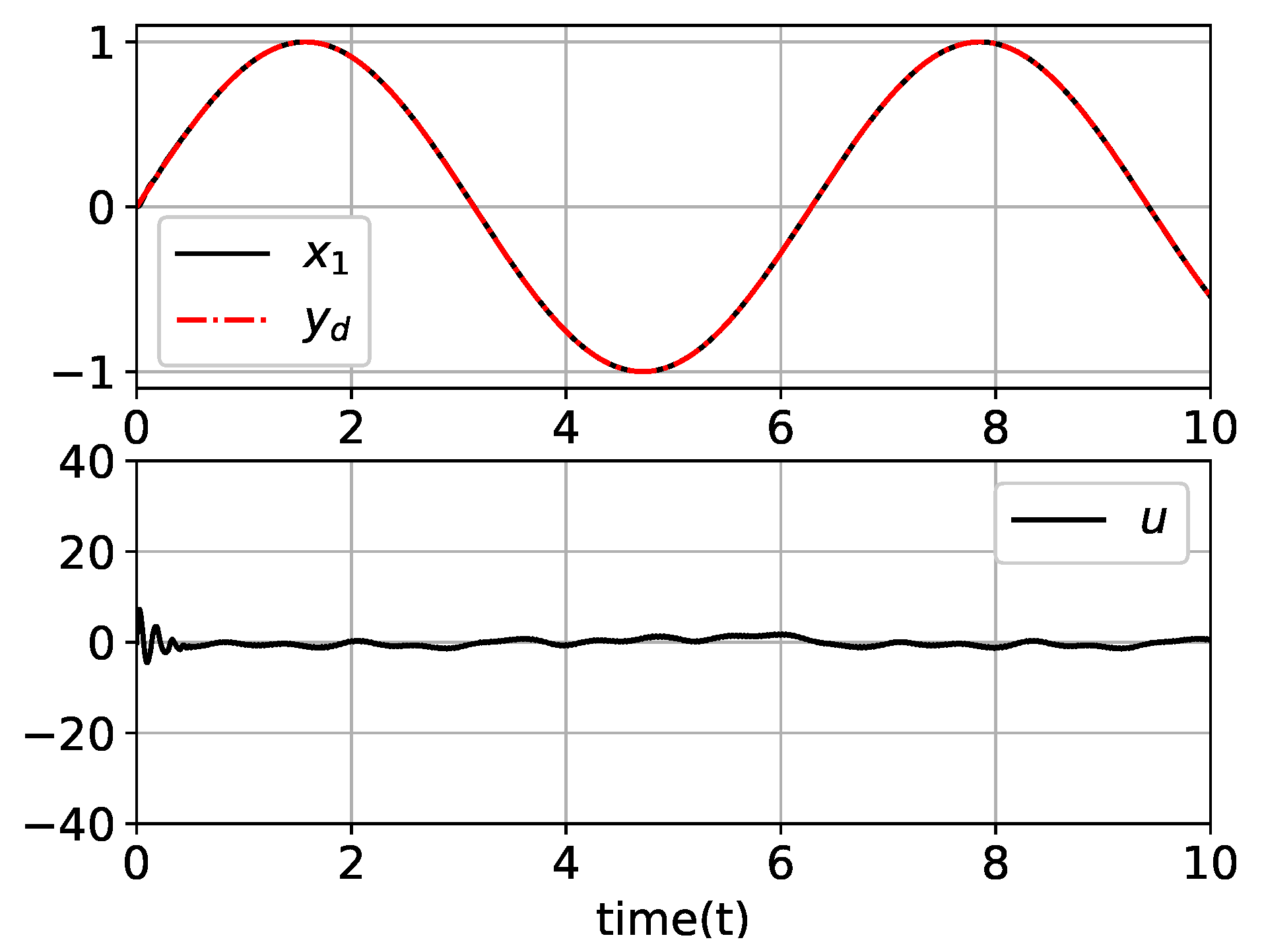
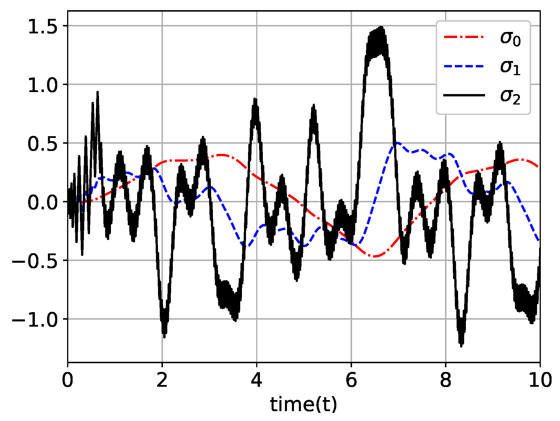
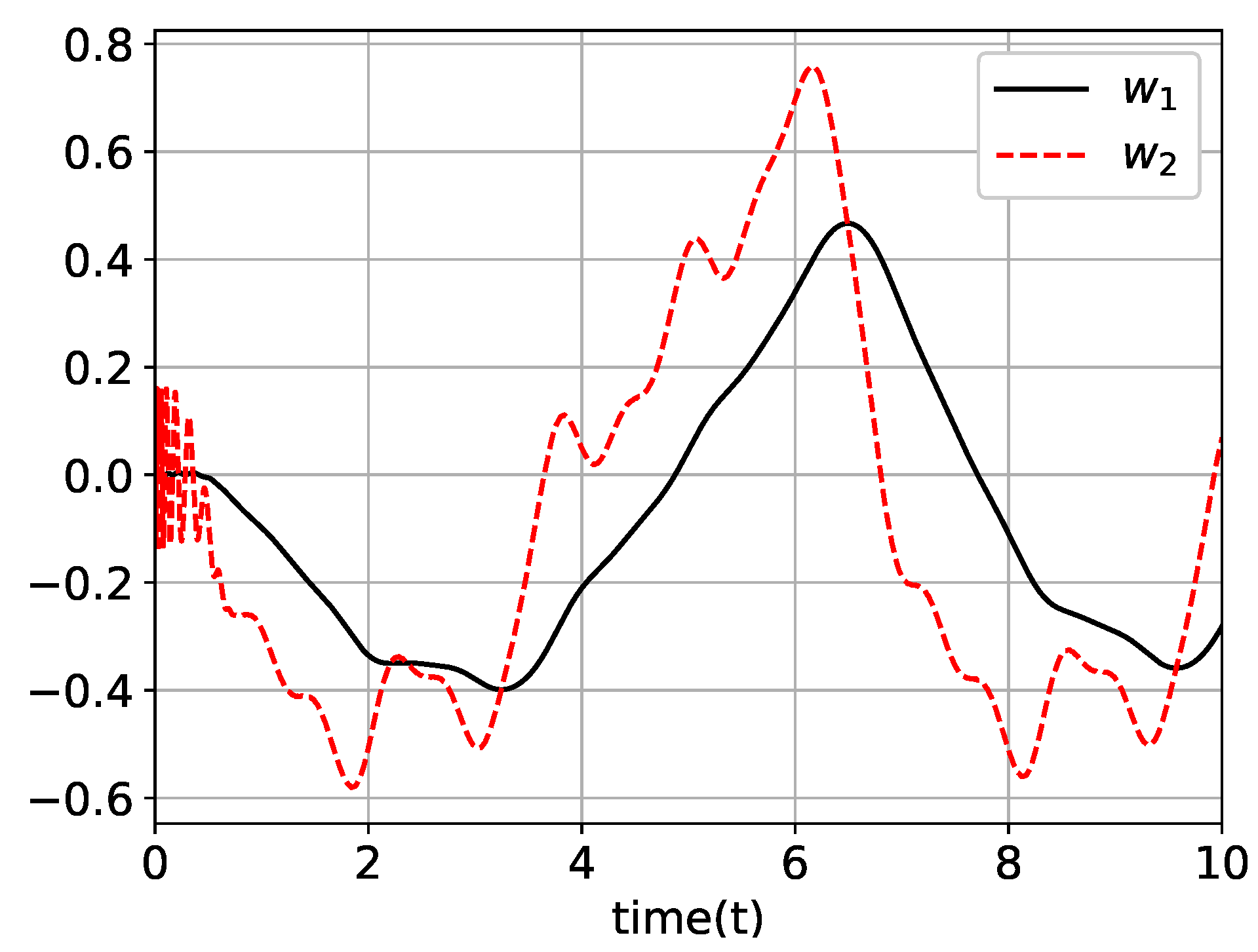
The simulation results are depicted in Figure 1, Figure 2 and Figure 3. It is illustrated that the output tracks $y_d$ very well after a short transient period in Figure 1. It is depicted in Figure 3 that there is a slight chattering in ${\sigma }_2$, which directly effects on the control input (39). From Figure 2 and Figure 3, all the states of the HOSM differentiator and input filter are bounded.

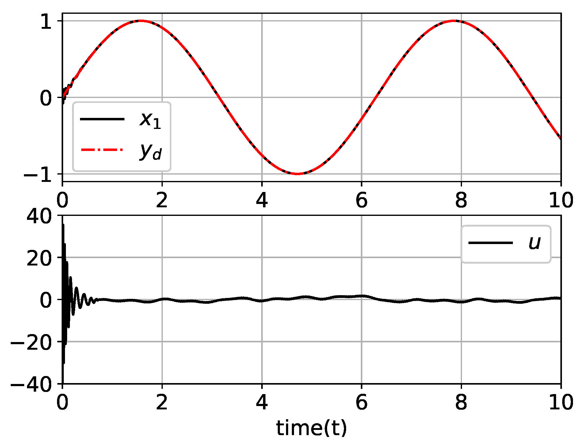
Additional simulation is performed for the different initial condition $\mathit{x}\left(0\right)={[0,0.1]}^T$ and the result is depicted in Figure 4. It is observed that the system output y tracks $y_d$ very well with smaller transient oscillation.

In both simulations, the control input is maintained within the range of $(-40,40)$. The states of HOSM differentiator and input filter are also bounded such that $|{\sigma }_i|<2$ for $i=1,2,3$ and $|w_i|<1.0$ for $i=1,2$ hold.

5. Conclusions

A novel output-feedback differentiator-based controller for SISO uncertain nonautonomous nonlinear pure-feedback systems is proposed. The HOSM differentiator, which is a finite-time exact differentiator, is used to estimate the time-derivatives of the signal which consist of the tracking error and filtered input. The controller has a very simple form and exponential convergence of the tracking error in finite time is guaranteed regardless of unstructured uncertainties and nonautonomous property in the considered system. No separate adaptive schemes, nor UAs such as NNs or FLSs that are to be adaptively tuned online to cope with system uncertainties, are required. Simulation results illustrate the simplicity and performance of the proposed controller.

References

- Wang, W.-Y.; Chan, M.-L.; Hsu, C.-C.J.; Lee, T.-T. H∞ Tracking-Based Sliding Mode Control for Unvertain Nonlinear Systems via an Adaptive Fuzzy-Neural Approach. IEEE Trans. Syst. Man Cybern. Part B Cybern. 2002, 32, 483–492. [Google Scholar] [CrossRef] [PubMed]
- Park, J.-H.; Park, G.-T. Robust adaptive fuzzy controller for nonlinear system Using Estimation of Bounds for Approximation Errors. Fuzzy Sets Syst. 2003, 133, 19–36. [Google Scholar] [CrossRef]
- Park, J.-H.; Park, G.-T. Robust Adaptive Fuzzy Controller for Nonaffine Nonlinear Systems with Dynamic Rule Activation. Int. J. Robust Nonliner Control 2003, 13, 117–139. [Google Scholar] [CrossRef]
- Park, J.-H.; Seo, S.-J.; Park, G.-T. Adaptive Fuzzy Observer with Minimal Dynamic Order for Uncertain Nonlinear Systems. IEE Proc. Control Theory Appl. 2003, 150, 189–197. [Google Scholar] [CrossRef]
- Park, J.-H.; Kim, S.-H. Direct Adaptive Output-Feedback Fuzzy Controller for Nonaffine Nonlinear System. IEE Proc. Control Theory Appl. 2004, 151, 65–72. [Google Scholar] [CrossRef]
- Park, J.-H.; Huh, S.-H.; Kim, S.-H.; Seo, S.-J.; Park, G.-T. Direct Adaptive Controller for Nonaffine Nonlinear Systems Using Self-Structuring Neural Networks. IEEE Trans. Neural Netw. 2005, 16, 414–422. [Google Scholar] [CrossRef]
- Park, J.-H.; Park, G.-T.; Kim, S.-H.; Moon, C.-J. Direct Adaptive Self-Structuring Fuzzy Controller for Nonaffine Nonlinear Systems. Fuzzy Sets Syst. 2005, 153, 429–445. [Google Scholar] [CrossRef]
- Park, J.-H.; Kim, S.-H.; Moon, C.-J. Adaptive Neural Control for Strict-Feedback Nonlinear Systems Without Backstepping. IEEE Trans. Neural Netw. 2009, 20, 1204–1209. [Google Scholar] [CrossRef]
- Yang, H.; Li, Z. Adaptive backstepping control for a class of semistrict feedback nonlinear systems using neural networks. J. Control Theory Appl. 2011, 9, 220–224. [Google Scholar] [CrossRef]
- Na, J.; Ren, X.; Zheng, D. Adaptive Control for Nonlinear Pure-Feedback Systems with High-Order Sliding Mode Observer. IEEE Trans. Neural Netw. Learn. Syst. 2013, 24, 370–382. [Google Scholar] [PubMed]
- Shen, Q.; Zhang, T.; Lim, C.-C. Novel Neural Control for a Class of Uncertain Pure-Feedback Systems. IEEE Trans. Neural Netw. Learn. Syst. 2014, 86, 912–922. [Google Scholar]
- Wang, H.; Chen, B.; Lin, C.; Sun, Y. Observer-based adaptive neural control for a class of nonlinear pure-feedback systems. Neurocomputing 2016, 171, 1517–1523. [Google Scholar] [CrossRef]
- Ge, S.S.; Wang, C. Adaptive NN control of uncertain nonlinear pure-feedback systems. Automatica 2002, 38, 671–682. [Google Scholar] [CrossRef]
- Zhao, Q.; Lin, Y. Adaptive dynamic surface control for pure-feedback systems. Int. J. Robust Nonlinear Control 2016, 22, 1647–1660. [Google Scholar] [CrossRef]
- Sun, G.; Wang, D.; Peng, Z.; Wang, H.; Lan, W.; Wang, M. Robust adaptive neural control of uncertain pure-feedback nonlinear systems. Int. J. Control 2013, 86, 912–922. [Google Scholar] [CrossRef]
- Du, H.; Shao, H.; Yao, P. Adaptive Neural Network Control for a Class of Low-Trangular-Structured Nonlinear Systems. IEEE Trans. Neural Netw. 2006, 17, 509–514. [Google Scholar] [CrossRef]
- Zhang, T.; Shi, X.; Zhu, Q.; Yang, Y. Adaptive neural tracking control of pure-feedback nonlinear systems with unknown gain signs and unmodeled dynamics. Neurocomputing 2013, 121, 290–297. [Google Scholar] [CrossRef]
- Chen, Z.; Ge, S.S.; Zhang, Y.; Li, Y. Adaptive Neural Control of MIMO Nonlinear Systems with a Block-Trangular Pure-Feedback Control Structure. IEEE Trans. Neural Netw. Learn. Syst. 2014, 25, 2017–2029. [Google Scholar] [CrossRef]
- Sun, G.; Wang, D.; Peng, Z. Adaptive control based on single neural network approximation for non-linear pure-feedback sustems. IET Control Theory Appl. 2012, 6, 2387–2396. [Google Scholar] [CrossRef]
- Wang, D. Neural network-based adaptive dynamic surface control of uncertain nonlinear pure-feedback systems. Int. J. Robust Nonlinear Control 2011, 21, 527–541. [Google Scholar] [CrossRef]
- Zhang, T.-P.; Zhu, Q.; Yang, Y.-Q. Adaptive neural control of non-affine pure-feedback non-linear systems with input nonlinearity and perturbed uncertainties. Int. J. Syst. Sci. 2012, 43, 691–706. [Google Scholar] [CrossRef]
- Park, J.-H.; Kim, S.-H.; Park, T.-S. Output-Feedback Adaptive Neural Controller for Uncertain Pure-Feedback Nonlinear Systems Using a High-Order Sliding Mode Observer. IEEE Trans. Neural Netw. Learn. Syst. 2019, 30, 1596–1601. [Google Scholar] [CrossRef] [PubMed]
- Hou, M.; Deng, Z.; Duan, G. Adaptive control of uncertain pure-feedback nonlinear systems. Int. J. Syst. Sci. 2017, 48, 2137–2145. [Google Scholar] [CrossRef]
- Liu, W.; Lim, C.C.; Shi, P.; Xu, S. Observer-based tracking control for MIMO pure-feedback nonlinear systems with time-delay and input quantisation. Int. J. Control 2017, 90, 2433–2448. [Google Scholar] [CrossRef]
- Tong, S.; Li, Y.; Shi, P. Observer-based adaptive fuzzy backstepping output feedback control of uncertain MIMO pure-feedback nonlinear systems. IEEE Trans. Fuzzy Syst. 2012, 20, 771–785. [Google Scholar] [CrossRef]
- Li, Y.; Tong, S.; Li, T. Adaptive Fuzzy Output Feedback Dynamic Surface Control of Interconnected Nonlinear Pure-Feedback Systems. IEEE Trans. Cybern. 2015, 45, 138–149. [Google Scholar] [CrossRef] [PubMed]
- Liu, Y.-J.; Lu, S.; Li, D.; Tong, S. Adaptive Controller Design-Based ABLF for a Class of Nonlinear Time-Varying State Constraint Systems. IEEE Trans. Syst. Man Cybern. Syst. 2017, 47, 1546–1553. [Google Scholar] [CrossRef]
- Liu, Y.-J.; Tong, S. Barrier Lyapunov functions for Nussbaum gain adaptive control of full state constraint nonlinear systems. Automatica 2017, 76, 143–152. [Google Scholar] [CrossRef]
- Levant, A. Higher-order sliding modes, differentiation and output-feedback control. Int. J. Control 2003, 76, 924–941. [Google Scholar] [CrossRef]
- Levant, A. Homegeneity approach to high-order sliding mode design. Automatica 2005, 41, 823–830. [Google Scholar] [CrossRef]
- Slotine, J.J.E.; Li, W. Applied Nonlinear Control; Prentice-Hall Inc.: Englewood Cliffs, NJ, USA, 1991. [Google Scholar]
- Park, J.-H.; Kim, S.-H.; Park, T.-S. Approximation-Free Output-Feedback Control of Uncertain Nonlinear Systems Using Higher-Order Sliding Mode Observer. J. Dyn. Syst. Meas. Control 2018, 140, 124502. [Google Scholar] [CrossRef]
- Hunter, J.D. Matplotlib: A 2D graphics environment. Comput. Sci. Eng. 2007, 9, 90–95. [Google Scholar] [CrossRef]
© 2019 by the authors. Licensee MDPI, Basel, Switzerland. This article is an open access article distributed under the terms and conditions of the Creative Commons Attribution (CC BY) license (http://creativecommons.org/licenses/by/4.0/).