Stability and Bifurcation Analysis on a Predator–Prey System with the Weak Allee Effect

Abstract

In this paper, the dynamics of a predator-prey system with the weak Allee effect is considered. The sufficient conditions for the existence of Hopf bifurcation and stability switches induced by delay are investigated. By using the theory of normal form and center manifold, an explicit expression, which can be applied to determine the direction of the Hopf bifurcations and the stability of the bifurcating periodic solutions, are obtained. Numerical simulations are performed to illustrate the theoretical analysis results.

1. Introduction

The Allee effect refers to the phenomenon that individuals of many species benefit from the presence of conspecifics, which implies when the per capita growth rate becomes bigger with the increase of the density and gets smaller as long as density passes through a critical value [1]. When the growth rate decreases but still keeps positive at a low population density, the Allee effect is called weak. It is easy to see that this situation is totally different from the logistic growth. During the last decade this phenomenon attracted a lot of attention with the rise of conservation biology.

The dynamics with the Allee effect, such as the stability of positive equilibrium [2,3,4,5,6,7], the existence of periodic solution [8,9,10,11,12], or bifurcation analysis [13,14,15], on nonlinear systems have been extensively investigated. Especially, Boukal and L. Berec [16] critically reviewed and classified models of single-species population dynamics with the demographic Allee effect. Meanwhile in consideration of the carrying capacity of environment with respect to the prey in the per capita growth rate of the population, they also proposed the following differential equation with the weak Allee effect

$$\dot{N}(t)=\frac{\epsilon }{K}{N}^2(t)\left(1-\frac{N(t)}{K}\right),$$

(1)

where $N(t)$ denotes the prey population at moment t, $0<\epsilon <1$ is the per capita growth rate of the population and $K>0$ is the carrying capacity of the environment. In biology, the group defense enriches the ability of the prey to defend or escape from the predators, and thus it helps decrease the predation. Tabares et al. [17] proposed the coupled system of equations

$$\begin{array}{c}\dot{N}(t)=\frac{4\epsilon }{K}{N}^2(t)\left(1-\frac{N(t)}{K}\right)-\alpha N(t)P(t),\hfill \\ \dot{P}(t)=-\gamma P(t)+a\beta P(t){\int }_{-\infty }^{t}N(\tau )exp(-a(t-\tau ))d\tau .\hfill \end{array}$$

(2)

as a model to describe the dynamical behaviour of the predator-prey system incorporating a weak Allee effect in the prey population $N(t)$ and a distributed delay in the predator populations $P(t)$ at time t. They analyzed the influence of weak Allee effect in the system. Here $\epsilon ,\alpha ,\beta ,\gamma ,a$ and K are all positive parameters. $\alpha$ is the rate of predation, $\beta$ is the conversion rate, $\gamma$ is the predator mortality in the absence of prey and a is the delay parameter. K denotes the carrying capacity of the environment with respect to the prey. Equation (2) is regarded as a predator-prey system with group defense [18]. J. D. Ferreira et al. [1] proposed the system

$$\begin{array}{c}\dot{N}(t)=\frac{4\epsilon }{K}{N}^2(t)\left(1-\frac{N(t)}{K}\right)-\alpha N(t)P(t),\hfill \\ \dot{P}(t)=-\gamma P(t)+\beta P(t){\int }_{-\infty }^{t}N(\tau )G(t-\tau )d\tau ,\hfill \end{array}$$

(3)

which describes the dynamics of interactions between a predator and a prey species with weak Allee effect. They studied the influence of the weak Allee effect with the density function $G:{\mathbb{R}}^{+}\to {\mathbb{R}}^{+}$ defined by

$$G(t)=a^{2}t{e}^{-at},a>0$$

and got analogous stability results as (2). For all biological processes in nature, the time delay is an inherent phenomenon. Hence, it is practical to assume that the growth rate of the prey population is determined by its recent history. So taking into account the maturation time of the prey, we define the density function $G(t)$ by

$$G(t)=a{e}^{-at},a>0,$$

and it makes system (2) the following delayed predator-prey model with weak Allee effect.

$$\begin{array}{c}\dot{N}(t)=\frac{4\epsilon }{K}{N}^2(t)\left(1-\frac{N(t-\tau )}{K}\right)-\alpha N(t)P(t),\hfill \\ \dot{P}(t)=-\gamma P(t)+a\beta P(t){\int }_{-\infty }^{t}N(\tau )exp(-a(t-\tau ))d\tau .\hfill \end{array}$$

(4)

In this paper, we study the effect of the delay $\tau$ on the positive equilibrium of system (4), and investigate the normal form for the Hopf bifurcation. In Section 2, stability of the equilibrium and existence of Hopf bifurcations are given. In Section 3, the direction and stability of the bifurcating periodic solutions of the system will be analyzed. Finally, in Section 4, numerical simulations are performed to illustrate our theoretical results.

2. Stability of the Equilibrium and Existence of Hopf Bifurcations

System (4) can be rewritten as

$$\begin{array}{c}\dot{N}(t)=\frac{4\epsilon }{K}{N}^2(t)\left(1-\frac{N(t-\tau )}{K}\right)-\alpha N(t)P(t),\hfill \\ \dot{P}(t)=-\gamma P(t)+\beta P(t)Q(t),\hfill \\ \dot{Q}(t)=a(N(t)-Q(t)),\hfill \end{array}$$

(5)

where

$$Q(t)=a{\int }_{-\infty }^{t}N(\tau )exp(-a(t-\tau ))d\tau .$$

Introducing $N=K{x}_1$, $P=K{x}_2$, $Q=K{x}_3$, $t=\frac{\overline{t}}{\epsilon }$ and then dropping the bar, system (5) becomes

$$\begin{array}{c}{\dot{x}}_1(t)=4x_1^2(t)(1-x_1(t-\tau ))-\frac{K\alpha }{\epsilon }{x}_1(t)x_2(t),\hfill \\ {\dot{x}}_2(t)=-\frac{\gamma }{\epsilon }{x}_2(t)+\frac{K\beta }{\epsilon }{x}_2(t)x_3(t),\hfill \\ {\dot{x}}_3(t)=\frac{a}{\epsilon }(x_1(t)-x_3(t)).\hfill \end{array}$$

(6)

When $\tau =0$, system (6) is system (3) in [17]. System (6) has only one positive equilibrium $E\left(\frac{\gamma }{\beta K},\frac{4\epsilon \gamma (\beta K-\gamma )}{\alpha {\beta }^2{K}^3},\frac{\gamma }{\beta K}\right)$. In [17], sufficient conditions, which guarantee the positive equilibrium is locally asymptotically stable for system (6) with $\tau =0$, have been given. We now recall some of their conclusions.

Lemma 1.

Equilibrium E of system (6) is locally asymptotically stable provided the following inequalities are satisfied

$$\begin{array}{c}\beta K-\gamma >0,\hfill \end{array}$$

(7)

$$\begin{array}{c}2\gamma -\beta K>0,\hfill \end{array}$$

(8)

$$\begin{array}{cc}\hfill \frac{a{\beta }^2{K}^2+4\gamma \epsilon (2\gamma -\beta K)}{{\beta }^2\epsilon K^2}\times & \frac{4a\gamma (2\gamma -\beta K)}{{\beta }^2\epsilon K^2}-\frac{4a{\gamma }^2(\beta K-\gamma )}{{\beta }^2{\epsilon }^2{K}^2}>0.\hfill \end{array}$$

(9)

Let $b=\frac{1}{\beta K}$, then Equations (7)–(9) are equivalent to

$$\frac{1}{2}<b\gamma <1,$$

(10)

$$a>\frac{\gamma [1-(\gamma +4\epsilon )b+16\epsilon \gamma b^2-16\epsilon {\gamma }^2{b}^3]}{2b\gamma -1}.$$

(11)

Denote the three curves on $\gamma -b$ plane $b\gamma =\frac{1}{2}$, $b\gamma =1$ and $a=\frac{\gamma [1-(\gamma +4\epsilon )b+16\epsilon \gamma b^2-16\epsilon {\gamma }^2{b}^3]}{2b\gamma -1}$ by $l_1,l_2$ and $l_3$, respectively. For the case when $a=0.2$, $\epsilon =0.15$, the three curves divide the first quadrant of the $\gamma -b$ plane into four regions $D_i,i=1,2,3,4$ (see Figure 1a). We know from Lemma 1 that the positive equilibrium of system (6) is stable when $\tau =0$.

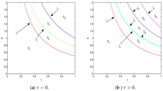
Figure 1. Bifurcation diagram of positive equilibrium in $\gamma$ –b plane for $a=0.2,\epsilon =0.15$.

The characteristic equation of system (6) at E is

$$\left|\begin{array}{ccc}\lambda -4b\gamma (1-b\gamma -b\gamma e^{-\lambda \tau })& \frac{\alpha Kb\gamma }{\epsilon }& 0\\ 0& \lambda & \frac{-4\gamma (1-b\gamma )}{\alpha K}\\ -\frac{a}{\epsilon }& 0& \lambda +\frac{a}{\epsilon }\end{array}\right|=0,$$

(12)

i.e.,

$${\lambda }^3+\left(\frac{a}{\epsilon }-4b\gamma (1-b\gamma )\right){\lambda }^2-\frac{4ab\gamma }{\epsilon }(1-b\gamma )\lambda +\frac{4ab{\gamma }^2(1-b\gamma )}{{\epsilon }^2}+4b^2{\gamma }^2\left({\lambda }^2+\frac{a}{\epsilon }\lambda \right)e^{-\lambda \tau }=0.$$

(13)

Clearly, $\lambda =0$ is not a root of (13). Let $\lambda =i\omega (\omega >0)$ be a root of (13), then

$$-i{\omega }^3-r_1{\omega }^2+i{r}_2\omega +r_3+r_4(-{\omega }^2+i\frac{a\omega }{\epsilon })e^{-i\omega \tau }=0,$$

(14)

where $r_1=\frac{a}{\epsilon }-4b\gamma (1-b\gamma )$, $r_2=-\frac{4ab\gamma }{\epsilon }(1-b\gamma )$, $r_3=\frac{4ab{\gamma }^2(1-b\gamma )}{{\epsilon }^2}$ and $r_4=4b^2{\gamma }^2$. Separating the real and imaginary parts leads to

$$\begin{array}{c}\hfill -r_1{\omega }^2+r_3+r_4\omega (-\omega cos(\omega \tau )+\frac{a}{\epsilon }sin(\omega \tau ))=0,\\ \hfill -{\omega }^3+r_2\omega +r_4\omega (\frac{a}{\epsilon }cos(\omega \tau )+\omega sin(\omega \tau ))=0.\end{array}$$

(15)

It follows directly from (15) that

$${\omega }^6+(r_1^2-2r_2-r_4^2){\omega }^4+(r_2^2-2r_1{r}_3-\frac{a^2{r}_4^2}{{\epsilon }^2}){\omega }^2+r_3^2=0.$$

(16)

In fact, (15) can be rewritten as

$$\begin{array}{c}\hfill -r_1{\omega }^2+r_3=-r_4\omega (-\omega cos(\omega \tau )+\frac{a}{\epsilon }sin(\omega \tau )),\\ \hfill -{\omega }^3+r_2\omega =-r_4\omega (\frac{a}{\epsilon }cos(\omega \tau )+\omega sin(\omega \tau )).\end{array}$$

Now, taking the square of two sides of the equations and adding we obtain (16) directly.

Let ${\omega }^2=z$, then (16) can be rewritten as

$$f(z)\equiv z^3+(r_1^2-2r_2-r_4^2)z^2+(r_2^2-2r_1{r}_3-\frac{a^2{r}_4^2}{{\epsilon }^2})z+r_3^2=0.$$

(17)

Since the constant term in (17) is positive, $f(z)=0$ has at least one positive root if and only if there exists $z^{*}>0$ such that

$$f^{{}^{\prime }}(z^{*})=0andf(z^{*})\le 0.$$

(18)

In fact,

$$f^{{}^{\prime }}(z)=3z^2+2Az+B,$$

where $A=r_1^2-2r_2-r_4^2$ and $B=r_2^2-2r_1{r}_3-\frac{a^2{r}_4^2}{{\epsilon }^2}$. When $B<0$, it is clearly that $f^{{}^{\prime }}(z)=0$ has a positive root $z^{*}=\frac{-A+\sqrt{A^2-3B}}{3}$. Through direct calculation, we get

$$B=\frac{8ab{\gamma }^2}{{\epsilon }^2}\left(2ab{(1-b\gamma )}^2-2a{b}^3{\gamma }^2-\frac{a}{\epsilon }(1-b\gamma )+4b\gamma {(1-b\gamma )}^2\right).$$

Thus, $B<0$ if

$$2ab{(1-b\gamma )}^2-2a{b}^3{\gamma }^2-\frac{a}{\epsilon }(1-b\gamma )+4b\gamma {(1-b\gamma )}^2<0.$$

(19)

We rewrite (19) as

$$a>\frac{4b\epsilon \gamma {(1-b\gamma )}^2}{1-b\gamma +2\epsilon b^3{\gamma }^2-2b\epsilon {(1-b\gamma )}^2}.$$

(20)

Denote $l_4:a=\frac{4b\epsilon \gamma {(1-b\gamma )}^2}{1-b\gamma +2\epsilon b^3{\gamma }^2-2b\epsilon {(1-b\gamma )}^2}$ and $l_5:f(z^{*})=0$, then curve $l_4$ divides $D_4$ into two regions $D_5$ and $D_6$, curve $l_5$ divides $D_3$ into two regions $D_7$ and $D_8$ (see Figure 1b). This means that Equation (17) has two positive roots in region $D_7$. Thus, we can draw the following conclusions.

Lemma 2.

Assume (10), (11), (18) and (20) hold,

(i) when $f(z^{*})=0$, $f(z)=0$ has one positive root;

(ii) when $f(z^{*})<0$, $f(z)=0$ has two positive roots.

A positive root of $f(z)=0$ corresponds to a pair of purely imaginary roots of Equation (3). Thus we get the following results.

Lemma 3.

Assume (10), (11), (18) and (20) hold.

(i) if $f(z)=0$ has one positive root $z^{*}$, then (16) has one pair of purely imaginary roots $\pm i{\omega }_0$ with double, where ${\omega }_0^2=z^{*}$;

(ii) if $f(z)=0$ has two positive roots $z_{+}$ and $z_{-}$, then (16) has two pair of purely imaginary roots $\pm i{\omega }_{+}$ and $\pm i{\omega }_{-}$, where ${\omega }_{+}^2=z_{+}$ and ${\omega }_{-}^2=z_{-}$. Furthermore $f^{{}^{\prime }}(z_{+})>0$ and $f^{{}^{\prime }}(z_{-})<0$.

Denote ${\omega }_{*}$ as a positive root of (16). By (15), we have

$$sin{\omega }_{*}\tau =\frac{{\omega }_{*}^4+\left(\frac{a}{\epsilon }{r}_1-r_2\right){\omega }_{*}^2-\frac{a}{\epsilon }{r}_3}{r_4{\omega }_{*}\left({\omega }_{*}^2+\frac{a^2}{{\epsilon }^2}\right)}.$$

(21)

$$cos{\omega }_{*}\tau =\frac{\left(\frac{a}{\epsilon }-r_1\right){\omega }_{*}^3+\left(r_3-\frac{a{r}_2}{\epsilon }\right){\omega }_{*}}{r_4{\omega }_{*}\left({\omega }_{*}^2+\frac{a^2}{{\epsilon }^2}\right)}\equiv G({\omega }_{*}).$$

(22)

Since $\frac{a}{\epsilon }-r_1=4b\gamma (1-b\gamma )>0$ and $r_3-\frac{a{r}_2}{\epsilon }=\frac{4ab\gamma }{{\epsilon }^2}(1-b\gamma )(\gamma +a)>0$, we known $cos{\omega }_{*}\tau >0$.

Let

$$h(z)=z^2+\left(\frac{a}{\epsilon }{r}_1-r_2\right)z-\frac{a}{\epsilon }{r}_3$$

(23)

Since ${(\frac{a}{\epsilon }{r}_1-r_2)}^2+\frac{4a}{\epsilon }{r}_3>0$ and $-\frac{a}{\epsilon }{r}_3<0$, then $h(z)=0$ has one positive root and one negative root. Denote the positive root by $z_0$. According to the discussions above and Ruan. S et al. [19], we get the following conclusion.

Lemma 4.

(i) If (10), (11), (18) and (20) are not all satisfied, then Equation (13) has at least one root with positive real part for $\tau >0$;

(ii) If (10), (11), (20) and $f(z^{*})=0$ hold, then there exists ${\tau }_0^{+}<{\tau }_1^{+}<\cdots <{\tau }_j^{+}<\cdots$, such that Equation (13) has a pair of purely imaginary roots $\pm i{\omega }_{+}$ with double when $\tau ={\tau }_j^{+}$;

(iii) If (10), (11), (20) and $f(z^{*})<0$ hold, then there exists ${\tau }_0^{+}<{\tau }_1^{+}<\cdots <{\tau }_j^{+}<\cdots$ and ${\tau }_0^{-}<{\tau }_1^{-}<\cdots <{\tau }_j^{-}<\cdots$ such that Equation (13) has a pair of purely imaginary roots $\pm i{\omega }_{\pm }$ when $\tau ={\tau }_j^{\pm }$, respectively, where

$${\tau }_j^{+}=\left\{\begin{array}{cc}\frac{1}{{\omega }_{+}}[arccosG({\omega }_{+})+2j\pi ],\hfill & z_0<z_{+},\hfill \\ \frac{1}{{\omega }_{+}}[-arccosG({\omega }_{+})+2(j+1)\pi ],\hfill & z_0>z_{+},\hfill \end{array}\right.$$

(24)

and

$${\tau }_j^{-}=\left\{\begin{array}{cc}\frac{1}{{\omega }_{-}}[-arccosG({\omega }_{-})+2(j+1)\pi ],\hfill & z_0>z_{-},\hfill \\ \frac{1}{{\omega }_{-}}[arccosG({\omega }_{-})+2j\pi ],\hfill & z_0<z_{-}.\hfill \end{array}\right.$$

(25)

Let $\lambda (\tau )=r(\tau )+i\omega (\tau )$ be the root of Equation (13) satisfying $r({\tau }_j^{\pm })=0$, $\omega ({\tau }_j^{\pm })={\omega }_{\pm }$, respectively. Substituting $\lambda (\tau )=r(\tau )+i\omega (\tau )$ into Equation (13) and taking derivative with respect to $\tau$, we get

$$\begin{array}{ccc}\frac{d\lambda }{d\tau }\hfill & =\hfill & \frac{\lambda r_4\left({\lambda }^2+\frac{a}{\epsilon }\lambda \right)e^{-\lambda \tau }}{3{\lambda }^2+2r_1\lambda +r_2+r_4\left(2\lambda +\frac{a}{\epsilon }\right)e^{-\lambda \tau }-r_4\tau \left({\lambda }^2+\frac{a}{\epsilon }\lambda \right)e^{-\lambda \tau }}\hfill \\ & =\hfill & \frac{r_4{\omega }^2\left[\left(\frac{a}{\epsilon }cos\omega \tau +\omega sin\omega \tau \right)+i\left(\omega cos\omega \tau -\frac{a}{\epsilon }sin\omega \tau \right)\right]}{H(\omega ,\tau )},\hfill \end{array}$$

(26)

where

$$\begin{array}{cc}\hfill H(\omega ,\tau )=& -3{\omega }^2+r_2+r_4\left[\left(\frac{a}{\epsilon }-{\omega }^2\tau \right)cos\omega \tau +\left(2\omega +\frac{a\omega \tau }{\epsilon }sin\omega \tau \right)\right]\\ & +i[2r_1\omega +r_4\left(\left(2\omega +\frac{a\omega \tau }{\epsilon }\right)cos\omega \tau +\left({\omega }^2\tau -\frac{a}{\epsilon }\right)sin\omega \tau \right],\end{array}$$

It follows that

$$\begin{array}{c}Re(\frac{d\lambda }{d\tau })=\frac{-{\omega }^2{r}_4}{\Delta }\times \hfill \\ \{\{-3{\omega }^2+r_2+r_4\left[\left(\frac{a}{\epsilon }-{\omega }^2\tau \right)cos\omega \tau +\left(2\omega +\frac{a\omega \tau }{\epsilon }sin\omega \tau \right)\right]\}(\frac{a}{\epsilon }cos\omega \tau +\omega sin\omega \tau )\hfill \\ +[2r_1\omega +r_4\left(\left(2\omega +\frac{a\omega \tau }{\epsilon }\right)cos\omega \tau +\left({\omega }^2\tau -\frac{a}{\epsilon }\right)sin\omega \tau \right]\left(\omega cos\omega \tau -\frac{a}{\epsilon }sin\omega \tau \right)\}\hfill \\ =\frac{-{\omega }^2}{\Delta }\left[-3{\omega }^4-2(r_1^2-2r_2-r_4){\omega }^2-(r_2^2-2r_1{r}_3-\frac{r_4^2{a}^2}{{\epsilon }^2})\right]\hfill \\ =\frac{-{\omega }^2}{\Delta }\left[-3z_{\pm }^2-2(r_1^2-2r_2-r_4)z_{\pm }-(r_2^2-2r_1{r}_3-\frac{r_4^2{a}^2}{{\epsilon }^2})\right]\hfill \\ =\frac{-{\omega }^2}{\Delta }{f}^{{}^{\prime }}(z_{\pm }),\hfill \end{array}$$

(27)

namely, $r^{{}^{\prime }}({\tau }_j^{+})<0$ and $r^{{}^{\prime }}({\tau }_j^{-})>0$ ($j=0,1,2,\cdots$ ), where $△=|H(\omega ,\tau )|$. Therefore, the transversality condition holds, and thus Hopf-bifurcation occurs at $\tau ={\tau }_j^{\pm }$. Furthermore, we have the following conclusion.

Lemma 5.

Assume (10), (11), (20) and (18) hold.

(i) For $f(z^{*})<0$, there exists a integer m such that

$${\tau }_0^{+}<{\tau }_0^{-}<{\tau }_1^{+}<{\tau }_1^{-}<\cdots <{\tau }_{m-1}^{-}<{\tau }_m^{+}<{\tau }_{m+1}^{+}<{\tau }_{m+1}^{-}.$$

Equation (13) has at least a pair of positive real parts when $\tau \in {\bigcup }_{j=0}^m({\tau }_j^{+},{\tau }_j^{-})$;

(ii) All roots of Equation (13) have negative real parts when $\tau \in {\bigcup }_{j=1}^m({\tau }_{j-1}^{-},{\tau }_j^{+})$; Equation (13) has at least a pair of roots with positive real parts when $\tau >{\tau }_m^{+}$.

(iii) when $\tau ={\tau }_j^{+}$ and $\tau ={\tau }_j^{-}(j=0,1,2,\cdots )$, all roots of Equation (13) have negative real parts except the purely imaginary roots $\pm i{\omega }_{+}$ and $\pm i{\omega }_{-}$.

From (24) and (25), it is easy to verify that

$${\tau }_0^{+}<{\tau }_0^{-},\mathrm{and}{\tau }_j^{+}-{\tau }_{j-1}^{+}<{\tau }_j^{-}-{\tau }_{j-1}^{-}.$$

Therefore, together with the define of ${\tau }_j^{\pm }$ and ${\omega }_{\pm }$, means that the lemma is true.

Now we have found the stability switches. In another words, the stability of the equilibrium switching from stability to instability when $\tau$ passes through ${\tau }_j^{+}(j=0,1,2,\cdots ,m)$ and back to stability when $\tau$ passes through ${\tau }_j^{-}(j=0,1,2,\cdots ,m-1)$. When $\tau >{\tau }_m^{+}$, the equilibrium is instability for ever.

3. Direction and Stability of Hopf Bifurcations

In Section 2, some conditions which guarantee system (5) and its modification (6) undergo Hopf bifurcation at some critical values of $\tau$ are obtained. We now apply the normal form and center manifold theory introduced by Hassard et al. [20] to study the direction of these Hopf bifurcations and stability of the bifurcated periodic solutions.

We rescale the time by $t\to \frac{t}{\tau }$ to normalize the delay. Let $\tau ={\tau }^{*}+\mu ,\mu \in \mathbb{R}$ and ${\tau }^{*}\in \left\{{\tau }_j^{+}\right\}\bigcup \left\{{\tau }_j^{-}\right\}$, then $\mu =0$ is the Hopf bifurcation value and system (6) is equivalent to the following functional differential equation in $C=C([-1,0],{\mathbb{R}}^3)$

$$\dot{x}(t)=L_{\mu }(x_t)+F(\mu ,x_t).$$

(28)

where $x_t(\theta )=x(t+\theta )\in C$, and $L_{\mu }:C\to {\mathbb{R}}^3$, $F:\mathbb{R}\times C\to {\mathbb{R}}^3$ are given respectively, by

$$\begin{array}{ccc}\hfill L_{\mu }(\varphi )& =& ({\tau }^{*}+\mu )\left(\begin{array}{ccc}{a}_{11}& a_{12}& 0\\ 0& 0& a_{23}\\ a_{31}& 0& a_{33}\end{array}\right)\left(\begin{array}{c}{\varphi }_1(0)\\ {\varphi }_2(0)\\ {\varphi }_3(0)\end{array}\right)\hfill \\ & +& ({\tau }^{*}+\mu )\left(\begin{array}{ccc}M& 0& 0\\ 0& 0& 0\\ 0& 0& 0\end{array}\right)\left(\begin{array}{c}{\varphi }_1(-1)\\ {\varphi }_2(-1)\\ {\varphi }_3(-1)\end{array}\right)\hfill \end{array}$$

(29)

and

$$F(\mu ,\varphi )=({\tau }^{*}+\mu )\left(\begin{array}{c}4(1-b\gamma ){\varphi }_1^2(0)-8{\varphi }_1(0){\varphi }_1(-1)-\frac{K\alpha }{\epsilon }{\varphi }_1(0){\varphi }_2(0)+h.o.t\\ \frac{K\beta }{\epsilon }{\varphi }_2(0){\varphi }_3(0)\\ 0\end{array}\right),$$

(30)

where $a_{11}=4b\gamma (1-b\gamma )$, $a_{12}=-\frac{K\alpha b\gamma }{\epsilon }$, $a_{13}=\frac{4\gamma (1-b\gamma )}{K\alpha }$, $a_{31}=\frac{a}{\epsilon }$, $a_{33}=-\frac{a}{\epsilon }$, and $M=-4b^2{\gamma }^2$.

By the Reisz representation theorem, there exist a function $\eta (\theta ,\mu )$ of bounded variation for $\theta \in [-1,0]$ such that

$$\begin{array}{ccc}\hfill L_{\mu }\varphi ={\int }_{-1}^{0}d\eta (\theta ,\mu )\varphi (\theta )& for& \varphi \in C.\hfill \end{array}$$

(31)

In fact, we can choose

$$\begin{array}{ccc}\hfill \eta (\theta ,\mu )& =& ({\tau }^{*}+\mu )\left(\begin{array}{ccc}{a}_{11}& a_{12}& 0\\ 0& 0& a_{23}\\ a_{31}& 0& a_{33}\end{array}\right)\delta (\theta )\hfill \\ & -& ({\tau }^{*}+\mu )\left(\begin{array}{ccc}M& 0& 0\\ 0& 0& 0\\ 0& 0& 0\end{array}\right)\delta (\theta +1),\hfill \end{array}$$

(32)

where

$$\delta (\theta )=\left\{\begin{array}{cc}0,& \theta \ne 0,\\ 1,& \theta =0.\end{array}\right.$$

For $\varphi \in C^1([-1,0],{\mathbb{R}}^3)$, define

$$\begin{array}{c}\hfill A(\mu )\varphi =\left\{\begin{array}{cc}\frac{d\varphi }{d\theta },\hfill & \theta \in [-1,0),\hfill \\ {\int }_{-1}^{0}d\eta (s,\mu )\varphi (s),\hfill & \theta =0,\hfill \end{array}\right.\end{array}$$

(33)

and

$$\begin{array}{c}\hfill R(\mu )\varphi =\left\{\begin{array}{cc}0,\hfill & \theta \in [-1,0),\hfill \\ F(\mu ,\varphi ),\hfill & \theta =0.\hfill \end{array}\right.\end{array}$$

(34)

Then (28) can be rewritten as

$$\dot{x}(t)=A(\mu )x_t+R(\mu )x_t.$$

(35)

For $\psi \in C^1([0,1],{({\mathbb{R}}^3)}^{*})$, define

$$\begin{array}{c}\hfill A^{*}\psi (s)=\left\{\begin{array}{cc}-\frac{d\psi }{ds},\hfill & s\in (0,1],\hfill \\ {\int }_{-1}^{0}d{\eta }^T(t,0)\psi (-t),\hfill & s=0.\hfill \end{array}\right.\end{array}$$

(36)

and a bilinear inner product

$$<\psi (s),\varphi (\theta )>=\overline{\psi }(0)\varphi (0)-{\int }_{-1}^0{\int }_{\xi }^{\theta }\overline{\psi }(\xi -\theta )d\eta (\theta )\varphi (\xi )d\xi ,$$

(37)

where $\eta (\theta )=\eta (\theta ,0)$. Then $A^{*}$ and $A(0)$ are adjoint operators, and $\pm i{\tau }^{*}{\omega }_{*}$ are eigenvalues of $A(0)$. Of course, they are also eigenvalues of $A^{*}$. Suppose that $q(\theta )=q(0)e^{i{\omega }_{*}{\tau }^{*}\theta }$ is an eigenvector of $A(0)$ corresponding to $i{\omega }_{*}{\tau }^{*}$, where $q(0)={(q_1,q_2,q_3)}^T$. From (31)–(33), we get

$$\begin{array}{c}\hfill {\tau }^{*}\left(\begin{array}{ccc}i{\omega }_{*}-a_{11}-M{e}^{-i{\omega }_{*}{\tau }^{*}}& -a_{12}& 0\\ 0& i{\omega }_{*}& -a_{23}\\ -a_{31}& 0& i{\omega }_{*}-a_{33}\end{array}\right)\left(\begin{array}{c}{q}_1\\ q_2\\ q_3\end{array}\right)=\left(\begin{array}{c}0\hfill \\ 0\hfill \\ 0\hfill \end{array}\right).\end{array}$$

(38)

Direct computation leads to

$$q_1=1,q_2=\frac{i{\omega }_{*}-a_{11}-M{e}^{-i{\omega }_{*}{\tau }^{*}}}{a_{12}},q_3=\frac{i{\omega }_{*}-a_{33}}{a_{31}}.$$

It is not difficult to verify that $q^{*}=D(q_1^{*},q_2^{*},q_3^{*})e^{-i{\omega }_{*}{\tau }^{*}\theta }$ is an eigenvector of $A^{*}$ corresponding to $-i{\omega }_{*}{\tau }^{*}$ such that $<q^{*},q>=1$, $<q^{*},\overline{q}>=0$, where

$$q_1^{*}=1,q_2^{*}=\frac{-a_{12}}{i{\omega }_{*}},q_3^{*}=\frac{-i{\omega }_{*}-a_{11}-M{e}^{i{\omega }_{*}{\tau }^{*}}}{a_{31}},\mathrm{and}D={[1+{\overline{q}}_2^{*}{q}_2+{\overline{q}}_3^{*}{q}_3+\tau M{e}^{i{\omega }_{*}{\tau }^{*}}]}^{-1}.$$

Using the same notations as in literatures [20,21,22,23], we shall compute the coordinates to describe the center manifold $C_0$ at $\mu =0$.

Let $x_t$ be the solution of (28) when $\mu =0$ and define

$$z(t)=<q^{*},x_t>,W(t,\theta )=x_t-z(t)q(\theta )-\overline{z}(t)\overline{q}(\theta )=x_t(\theta )-2Re\left\{z(t)q(\theta )\right\}.$$

On the center manifold $C_0$, we have

$$W(t,\theta )=W(z(t),\overline{z}(t),\theta ),$$

where

$$W(z(t),\overline{z}(t),\theta )=W_{20}(\theta )\frac{z^2}{2}+W_{11}(\theta )z\overline{z}+W_{02}(\theta )\frac{{\overline{z}}^2}{2}+\cdots ,$$

(39)

$z(t)$ and $\overline{z}(t)$ are local coordinates of center manifold $C_0$ in the direction of the q and $q^{*}$, respectively. According to the center manifold theory, we have

$$W(0,0,\theta )=0,W^{{}^{\prime }}(0,0,\theta )=0.$$

For solution $x_t$ in $C_0$ of Equation (28),

$$<\psi ,A\varphi >=<A^{*}\psi ,\varphi >,\mathrm{for}(\varphi ,\psi )\in D(A)\times D(A^{*})\mathrm{since}\mu =0,$$

so we have

$$\begin{array}{ccc}\hfill \dot{z}(t)& =& <q^{*},\dot{x}(t)>=<q^{*},L_{\mu }(x_t)+F(\mu ,x_t)>\hfill \\ & =& <q^{*},i{\omega }_{*}{\tau }^{*}{x}_t>+<q^{*},F(0,W+2Re\{(z(t)q(\theta )\})>\hfill \\ & =& i{\omega }_{*}\tau *z_t+{\overline{q}}^{*}(0)F(0,W(z,\overline{z},0))+2Re\{(z(t)q(0)\})\hfill \\ & \stackrel{\mathrm{def}}{=}& i{\omega }_{*}\tau *z_t+{\overline{q}}^{*}(0)F_0(z,\overline{z}).\hfill \end{array}$$

(40)

Consider the formal Taylor expansion of the $F_0(z,\overline{z})$ as follows

$$F_0(z,\overline{z})=F_{z^2}\frac{z^2}{2}+F_{\overline{z}}\frac{{\overline{z}}^2}{2}+F_{z\overline{z}}z\overline{z}+F_{z^2\overline{z}}\frac{z^2\overline{z}}{2}+\cdots$$

(41)

We rewrite (40) as

$$\dot{z}(t)=i{\omega }_{*}\tau *z(t)+g(z,\overline{z}),$$

(42)

where

$$g(z,\overline{z})={\overline{q}}^{*}(0)F_0(z,\overline{z})=g_{20}\frac{z^2}{2}+g_{11}z\overline{z}+g_{02}\frac{{\overline{z}}^2}{2}+g_{21}\frac{z^2\overline{z}}{2}+\cdots$$

(43)

According to (30), we have

$$\begin{array}{c}g(z,\overline{z})=\overline{D}{\tau }^{*}(1,\overline{q_2^{*}},\overline{q_3^{*}})\left(\begin{array}{c}{l}_{11}{\varphi }_1^2(0)+l_{12}{\varphi }_1(0){\varphi }_2(0)+l_{13}{\varphi }_1(0){\varphi }_1(-1)+l_{14}{\varphi }_1^2(0){\varphi }_1(-1)\\ l_{21}{\varphi }_2(0){\varphi }_3(0)\\ 0\end{array}\right)\\ =\overline{D}{\tau }^{*}\{(l_{11}+l_{12}{q}_2+l_{13}{e}^{-i{\omega }_{*}{\tau }^{*}}+l_{21}{q}_2{q}_3\overline{q_2^{*}})z^2+\\ [2l_{11}+l_{12}(q_2+{\overline{q}}_2)+l_{21}{\overline{q}}_2^{*}(q_2{\overline{q}}_3+{\overline{q}}_2{q}_3)]z\overline{z}+(l_{11}+l_{12}{\overline{q}}_2+l_{13}{e}^{i{\omega }_{*}{\tau }^{*}}+l_{21}{\overline{q}}_2^{*}{\overline{q}}_2{\overline{q}}_3){\overline{z}}^2\\ +[l_{11}(2W_{11}^{(1)}(0)+W_{20}^{(1)}(0))+l_{12}(W_{11}^{(2)}(0)+\frac{W_{20}^{(1)}(0)q_{12}}{2}+\frac{W_{20}^{(2)}(0)}{2}+W_{11}^{(1)}(0)q_{12})+l_{13}(W_{11}^{(1)}(-1)\\ +\frac{W_{20}^{(1)}(-1)}{2}+W_{20}^{(1)}(0)e^{i{\omega }_{*}{\tau }^{*}}+W_{11}^{(1)}(0)e^{-i{\omega }_{*}{\tau }^{*}})+l_{14}(e^{i{\omega }_{*}{\tau }^{*}}+2e^{-i{\omega }_{*}{\tau }^{*}})\\ +{\overline{q}}_2^{*}{l}_{21}(q_2{W}_{11}^{(3)}(0)+{\overline{q}}_2{W}_{20}^{(3)}(0)+{\overline{q}}_3{W}_{20}^{(2)}(0)+q_3{W}_{11}^{(2)}(0))\left]z^2\overline{z}\right\}.\end{array}$$

(44)

Comparing the coefficients with (43), we have

$$\begin{array}{ccc}\hfill g_{20}& =& 2\overline{D}{\tau }^{*}(l_{11}+l_{12}{q}_2+l_{13}{e}^{-i{\omega }_{*}{\tau }^{*}}+l_{21}{q}_2{q}_3\overline{q_2^{*}}),\hfill \\ \hfill g_{11}& =& \overline{D}{\tau }^{*}(2l_{11}+l_{12}(q_2+{\overline{q}}_2)+l_{13}(e^{-i{\omega }_{*}{\tau }^{*}}+e^{i{\omega }_{*}{\tau }^{*}})+l_{21}{\overline{q}}_2^{*}(q_2{\overline{q}}_3+{\overline{q}}_2{q}_3)),\hfill \\ \hfill g_{02}& =& 2\overline{D}{\tau }^{*}(l_{11}+l_{12}{\overline{q}}_2+l_{13}{e}^{i{\omega }_{*}{\tau }^{*}}+l_{21}{\overline{q}}_2^{*}{\overline{q}}_2{\overline{q}}_3),\hfill \\ \hfill g_{21}& =& 2\overline{D}{\tau }^{*}[l_{11}(2W_{11}^{(1)}(0)+W_{20}^{(1)}(0))+l_{12}(W_{11}^{(2)}(0)+\frac{W_{20}^{(1)}(0)q_{12}}{2}+\frac{W_{20}^{(2)}(0)}{2}\hfill \\ & +& W_{11}^{(1)}(0)q_{12})+l_{13}(W_{11}^{(1)}(-1)+\frac{W_{20}^{(1)}(-1)}{2}+W_{20}^{(1)}(0)e^{i{\omega }_{*}{\tau }^{*}}+W_{11}^{(1)}(0)e^{-i{\omega }_{*}{\tau }^{*}})\hfill \\ & +& l_{14}(e^{i{\omega }_{*}{\tau }^{*}}+2e^{-i{\omega }_{*}{\tau }^{*}})+{\overline{q}}_2^{*}{l}_{21}(q_2{W}_{11}^{(3)}(0)+{\overline{q}}_2{W}_{20}^{(3)}(0)+{\overline{q}}_3{W}_{20}^{(2)}(0)+q_3{W}_{11}^{(2)}(0))].\hfill \end{array}$$

In order to determine $g_{21}$, we focus on the computation of $W_{20}(\theta )$ and $W_{11}(\theta )$. By (35), we have

$$\begin{array}{c}\hfill \dot{W}={\dot{x}}_t-\dot{z}(t)q(\theta )-\dot{\overline{z}}(t)\overline{q}(\theta )=\left\{\begin{array}{cc}AW-gq(\theta )-\overline{g}\overline{q}(\theta ),\hfill & \theta \in [-1,0),\hfill \\ AW-gq(\theta )-\overline{g}\overline{q}(\theta )+F(\mu ,\varphi ),\hfill & \theta =0.\hfill \end{array}\right.\end{array}$$

(45)

Differentiating (39) with respect to t, we obtain

$$\begin{array}{ccc}\hfill \dot{W}& =& W_z\dot{z}+W_{\overline{z}}\dot{\overline{z}}\hfill \\ & =& [W_{20}(\theta )z+W_{11}(\theta )\overline{z}]\dot{z}+[W_{11}(\theta )z+W_{02}(\theta )\overline{z}]\dot{\overline{z}}+\cdots \hfill \\ & =& [W_{20}(\theta )z+W_{11}(\theta )\overline{z}](i{\omega }_{*}\tau *z+g(z,\overline{z}))\hfill \\ & & +[W_{11}(\theta )z+W_{02}(\theta )\overline{z}](i{\omega }_{*}\tau *\overline{z}+\overline{g}(z,\overline{z}))+\cdots \hfill \end{array}$$

(46)

Substituting (43) and (46) into (45), and comparing the coefficients, we have

$$\begin{array}{c}\hfill (2i{\omega }_{*}{\tau }^{*}-A)W_{20}(\theta )=\left\{\begin{array}{cc}-g_{20}q(\theta )-{\overline{g}}_{02}\overline{q}(\theta ),\hfill & \theta \in [-1,0),\hfill \\ -g_{20}q(0)-{\overline{g}}_{02}\overline{q}(0)+F_{z^2},\hfill & \theta =0.\hfill \end{array}\right.\end{array}$$

(47)

and

$$\begin{array}{c}\hfill -A{W}_{11}(\theta )=\left\{\begin{array}{cc}-g_{11}q(\theta )-{\overline{g}}_{11}\overline{q}(\theta ),\hfill & \theta \in [-1,0),\hfill \\ -g_{11}q(0)-{\overline{g}}_{11}\overline{q}(0)+F_{z\overline{z}},\hfill & \theta =0.\hfill \end{array}\right.\end{array}$$

(48)

According to (33) and (47), for $\theta \in [-1,0)$,

$$W_{20}^{{}^{\prime }}(\theta )=2i{\omega }_{*}{\tau }^{*}{W}_{20}(\theta )+g_{20}q(\theta )+{\overline{g}}_{02}\overline{q}(\theta ).$$

It is clear that the solution of above equation is

$$W_{20}(\theta )=\frac{i{g}_{20}}{{\omega }_{*}{\tau }^{*}}q(0)e^{i{\omega }_{*}{\tau }^{*}\theta }+\frac{i{\overline{g}}_{02}}{3{\omega }_{*}{\tau }^{*}}\overline{q}(0)e^{-i{\omega }_{*}{\tau }^{*}\theta }+E_1{e}^{2i{\omega }_{*}\theta }.$$

(49)

For $\theta =0$, we see from (47) that

$${\int }_{-1}^0{d}_{\theta }\eta (0,\theta )W_{20}=2i{\omega }_{*}{\tau }^{*}{W}_{20}(0)+g_{20}q(0)+{\overline{g}}_{02}\overline{q}(0)-F_{z^2}.$$

(50)

Substituting (49) into (50), we have

$$\begin{array}{c}\hfill \left((2i{\omega }_{*}{\tau }^{*}I-{\int }_{-1}^0{d}_{\theta }\eta (\theta )e^{2i{\omega }_{*}{\tau }^{*}\theta }\right)E_1=2{\tau }^{*}\left(\begin{array}{c}{l}_{11}+l_{12}{q}_{12}+l_{13}{e}^{-i{\omega }_{*}{\tau }^{*}}\\ l_{21}{\overline{q}}_2^{*}{q}_2{q}_3\\ 0\end{array}\right),\end{array}$$

(51)

namely,

$$\begin{array}{c}\hfill \left(\begin{array}{ccc}2i{\omega }_{*}-a_{11}-M{e}^{-2i{\omega }_{*}{\tau }^{*}\theta }& -a_{12}& 0\\ 0& 2i{\omega }_{*}& -a_{13}\\ -a_{31}& 0& 2i{\omega }_{*}-a_{33}\end{array}\right)E_1=2\left(\begin{array}{c}{l}_{11}+l_{12}{q}_{12}+l_{13}{e}^{-i{\omega }_{*}{\tau }^{*}}\\ l_{21}{\overline{q}}_2^{*}{q}_2{q}_3\\ 0\end{array}\right).\end{array}$$

(52)

So we have

$$\begin{array}{c}\hfill E_1^{(1)}=\frac{2}{M_1^{*}}\left|\begin{array}{ccc}{l}_{11}+l_{12}{q}_2+l_{13}{e}^{-i{\omega }_{*}{\tau }^{*}}& -a_{12}& 0\\ l_{21}{\overline{q}}_2^{*}{q}_2{q}_3& 2i{\omega }_{*}& -a_{13}\\ 0& 0& 2i{\omega }_{*}-a_{33}\end{array}\right|,\end{array}$$

$$\begin{array}{c}\hfill E_2^{(1)}=\frac{2}{M_1^{*}}\left|\begin{array}{ccc}2i{\omega }_{*}-a_{11}-M{e}^{-2i{\omega }_{*}{\tau }^{*}\theta }& l_{11}+l_{12}{q}_2+l_{13}{e}^{-i{\omega }_{*}{\tau }^{*}}& 0\\ 0& l_{21}{\overline{q}}_2^{*}{q}_2{q}_3& -a_{13}\\ -a_{31}& 0& 2i{\omega }_{*}-a_{33}\end{array}\right|,\end{array}$$

$$\begin{array}{c}\hfill E_3^{(1)}=\frac{2}{M_1^{*}}\left|\begin{array}{ccc}2i{\omega }_{*}-a_{11}-M{e}^{-2i{\omega }_{*}{\tau }^{*}\theta }& -a_{12}& l_{11}+l_{12}{q}_2+l_{13}{e}^{-i{\omega }_{*}{\tau }^{*}}\\ 0& 2i{\omega }_{*}& l_{21}{\overline{q}}_2^{*}{q}_2{q}_3\\ -a_{31}& 0& 0\end{array}\right|,\end{array}$$

where

$$\begin{array}{c}\hfill M_1^{*}=\left|\begin{array}{ccc}2i{\omega }_{*}-a_{11}-M{e}^{-2i{\omega }_{*}{\tau }^{*}\theta }& -a_{12}& 0\\ 0& 2i{\omega }_{*}& -a_{13}\\ -a_{31}& 0& 2i{\omega }_{*}-a_{33}\end{array}\right|.\end{array}$$

Similarly, we have

$$\begin{array}{c}\hfill E_1^{(2)}=\frac{2}{M_2^{*}}\left|\begin{array}{ccc}2l_{11}+l_{12}(q_2+{\overline{q}}_2)+l_{13}(e^{-i{\omega }_{*}{\tau }^{*}}+e^{i{\omega }_{*}{\tau }^{*}})& a_{12}& 0\\ l_{21}{\overline{q}}_2^{*}(q_2{\overline{q}}_3+{\overline{q}}_2{q}_3)& 0& a_{13}\\ 0& 0& a_{33}\end{array}\right|,\end{array}$$

$$\begin{array}{c}\hfill E_2^{(2)}=\frac{2}{M_2^{*}}\left|\begin{array}{ccc}{a}_{11}-M& 2l_{11}+l_{12}(q_2+{\overline{q}}_2)+l_{13}(e^{-i{\omega }_{*}{\tau }^{*}}+e^{i{\omega }_{*}{\tau }^{*}})& 0\\ 0& l_{21}{\overline{q}}_2^{*}(q_2{\overline{q}}_3+{\overline{q}}_2{q}_3)& a_{13}\\ 0& 0& a_{33}\end{array}\right|,\end{array}$$

$$\begin{array}{c}\hfill E_3^{(2)}=\frac{2}{M_2^{*}}\left|\begin{array}{ccc}{a}_{11}-M& a_{12}& 2l_{11}+l_{12}(q_2+{\overline{q}}_2)+l_{13}(e^{-i{\omega }_{*}{\tau }^{*}}+e^{i{\omega }_{*}{\tau }^{*}})\\ 0& 0& l_{21}{\overline{q}}_2^{*}(q_2{\overline{q}}_3+{\overline{q}}_2{q}_3)\\ a_{31}& 0& 0\end{array}\right|,\end{array}$$

where

$$\begin{array}{c}\hfill M_2^{*}=\left|\begin{array}{ccc}{a}_{11}-M& a_{12}& 0\\ a_{31}& 0& a_{13}\\ 0& 0& a_{33}\end{array}\right|.\end{array}$$

Thus, $g_{12}$ can be determined by the parameters and delay. So the following quantities can be derived:

$$C_1(0)=\frac{i}{2{\omega }_{*}{\tau }^{*}}(g_{20}{g}_{11}-2{\left|g_{11}\right|}^2-\frac{1}{3}{\left|g_{02}\right|}^2)+\frac{g_{12}}{2}.$$

$${\mu }_2=-\frac{Re\left\{C_1(0)\right\}}{Re\left\{{\lambda }^{{}^{\prime }}({\tau }^{*})\right\}},{\beta }_2=2Re\left\{C_1(0)\right\}.$$

$$T_2=-\frac{Im(C_1(0))+{\mu }_{2}Im{\lambda }^{{}^{\prime }}({\tau }^{*})}{{\tau }^{*}{\omega }_{*}}.$$

It is well-known from [20] that the sign of ${\mu }_2$ decides the direction of Hopf bifurcation, the sign of ${\beta }_2$ determines the stability of bifurcating periodic solutions and $T_2$ defines the period of bifurcating periodic solutions. Thus we have the following conclusion.

Theorem 1.

(1) The Hopf bifurcation is supercritical (subcritical) and the bifurcating periodic solutions exist for $\tau >{\tau }^{*}(\tau <{\tau }^{*})$ if ${\mu }_2>0({\mu }_2<0)$;

(2) The bifurcating periodic solutions are stable (unstable) if ${\beta }_2<0({\beta }_2>0)$;

(3) The periodic of the bifurcating periodic solutions increase (decrease) if $T_2>0(T_2<0)$.

4. Numerical Simulations

In this section, we perform some numerical simulations to verify our theoretical analysis proved in previous sections. To investigate the effect of delay, we focus on the case when $(\gamma ,b)\in D_7$. Set $a=0.2$, $\epsilon =0.15$, $\gamma =0.55$, $b=1.6$, $K=12.5$, $\beta =0.05$ and $\alpha =0.1$. By direct computation, we get ${\tau }_0^{+}\approx 0.4414$ and the equilibrium E is $(0.88,0.0507,0.88)$.

(i) Take $\tau =0.4$. Starting from the initial value $(x_1(0),x_2(0),x_3(0))=(0.2,0.05,0.2)$, we get Figure 2. According the previous analysis, the equilibrium should be stable. The simulation results coincide exactly with the our conclusion.

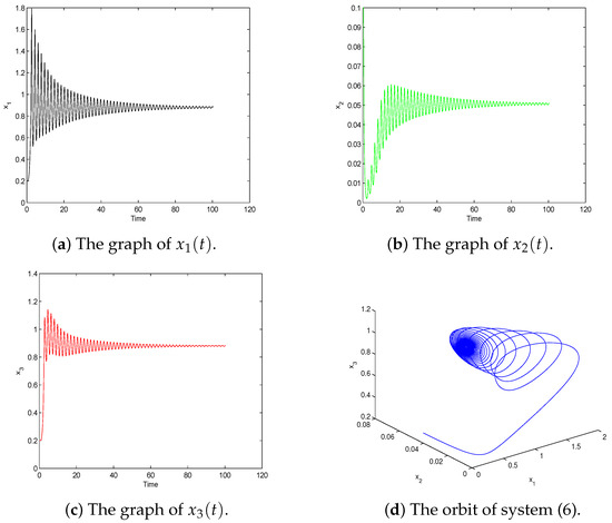
Figure 2. Behavior of system (6) with $\tau =0.4$. The positive equilibrium E is asymptotically stable when $\tau <{\tau }_0^{+}\approx 0.4414$.

(ii) Take $\tau =0.45$. Starting from the initial value $(x_1(0),x_2(0),x_3(0))=(0.8,0.05,0.8)$, we get Figure 3. This implies that the Hopf bifurcation associated with the critical value ${\tau }_0^{+}\approx 0.4414$ is supercritical, the bifurcating periodic solution is stable, and the equilibrium E is unstable. All these results are consistent with our analysis.

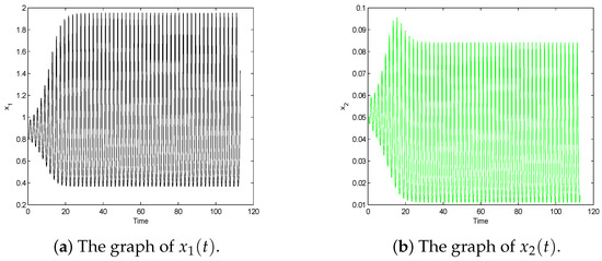
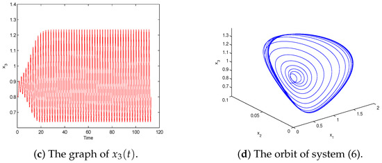
Figure 3. Behavior of system (6) with $\tau =0.45$. The positive equilibrium E is unstable. Furthermore, a periodic solution bifurcates from the positive equilibrium and is orbitally asymptotically stable.

(iii) Take $\tau =0.55$. Starting from the initial value $(x_1(0),x_2(0),x_3(0))=(0.8,0.05,0.8)$, we get Figure 4. In this case, the bifurcating periodic solution vanishes, but the equilibrium is still unstable.

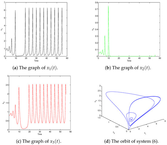
Figure 4. Behavior of system (6) with $\tau =0.55$. The positive equilibrium E is unstable when $\tau >{\tau }_0^{+}\approx 0.4414$.

5. Conclusions

In this paper, we have studied the dynamics of a predator-prey system with the weak Allee effect. Firstly, we investigated the effect of the time delay $\tau$ on the stability of the positive equilibrium of system (5). Then, by using the normal form and center manifold theorems, we explored the existence of the stability switches, the Hopf bifurcation, the bifurcating direction and the stability of the bifurcating periodic solutions when the characteristic equation of system (6) has two pairs of purely imaginary roots. Meanwhile, we found the characteristic equation of system (6) has one pair of purely imaginary roots which are double roots when $f(z)=0$ has one positive root. We believe system (6) perhaps has more interesting dynamics in this case which is more complicated than our present work and will be considered in the future. Furthermore, we can incorporate other time delays, such as predator maturation time, etc., into the mathematical model to investigate their dynamics by other methods, from which we may be able to obtain more interesting results.

References

- Ferreira, J.D.; Salazarb, C.A.T.; Tabares, P.C.C. Weak Allee effect in a predator-prey model involving memory with a hump. Nonlinear Anal.-Real World Appl. 2013, 14, 536–548. [Google Scholar] [CrossRef]
- Yang, K.; Miao, Z.; Chen, F.; Xie, X. Influence of single feedback control variable on an autonomous Holling-II type cooperative system. J. Math. Anal. Appl. 2016, 435, 874–888. [Google Scholar] [CrossRef]
- Lin, Q. Dynamic behaviors of a commensal symbiosis model with non-monotonic functional response and non-selective harvesting in a partial closure. Commun. Math. Biol. Neurosci. 2018, 2018, 4. [Google Scholar]
- Chen, F.; Wu, H.; Xie, X. Global attractivity of a discrete cooperative system incorporating harvesting. Adv. Differ. Equ. 2016, 2016, 268. [Google Scholar] [CrossRef][Green Version]
- Manna, D.; Maiti, A.; Samanta, G.P. A Michaelis-Menten type food chain model with strong Allee effect on the prey. Appl. Math. Comput. 2017, 311, 390–409. [Google Scholar] [CrossRef]
- Li, Y.N.; Li, Y.; Liu, Y.; Cheng, H. Stability Analysis and Control Optimization of a Prey-Predator Model with Linear Feedback Control. Discrete Dyn. Nat. Soc. 2018, 2018, 4945728. [Google Scholar] [CrossRef]
- Bai, Y.; Mu, X. Global asymptotic stability of a generalized SIRS epidemic model with transfer from infectious to susceptible. J. Appl. Anal. Comput. 2018, 8, 402–412. [Google Scholar]
- Han, M.; Zhang, L.; Wang, Y.; Khalique, C.M. The effects of the singular lines on the traveling wave solutions of modified dispersive water wave equations. Nonlinear Anal.-Real World Appl. 2019, 47, 236–250. [Google Scholar] [CrossRef]
- Ding, H.; Lim, C.W.; Chen, L.Q. Nonlinear vibration of a traveling belt with non-homogeneous boundaries. J. Sound Vib. 2018, 424, 78–93. [Google Scholar] [CrossRef]
- Zhang, L.; Wang, Y.; Khlique, C.M.; Bai, Y. Peakon and cuspon solutions of a generalized Camassa-Holm-Novikov equation. J. Appl. Anal. Comput. 2018, 8, 1938–1958. [Google Scholar]
- Li, T.; Lin, Q.; Chen, J. Positive periodic solution of a discrete commensal symbiosis model with Holling II functional response. Commun. Math. Biol. Neurosci. 2016, 2016, 22. [Google Scholar]
- Li, Y.; Cheng, H.; Wang, J.; Wang, Y. Dynamic analysis of unilateral diffusion Gompertz model with impulsive control strategy. Adv. Differ. Equ. 2018, 1, 32. [Google Scholar] [CrossRef]
- Bai, Y.; Li, Y. Stability and Hopf bifurcation for a stage-structured predator-prey model incorporating refuge for prey and additional food for predator. Adv. Differ. Equ. 2019, 2019, 42. [Google Scholar] [CrossRef]
- Shi, Z.; Wang, J.; Li, Q.; Cheng, H. Control optimization and homoclinic bifurcation of a prey-predator model with ratio-dependent. Adv. Differ. Equ. 2019, 2019, 2. [Google Scholar] [CrossRef]
- Huang, J.; Gong, Y.; Ruan, S. Bifurcation Analysis in a Predator-prey Model with Constant-yield Predator Harvesting. Disc. Cont. Dyn. Syst.-Ser. B 2013, 18, 2101–2121. [Google Scholar] [CrossRef]
- Boukal, D.; Berec, L. Single-species models of the Allee effect: Extinction boundaries, sex ratios and mate enconunters. J. Theor. Biol. 2002, 218, 375–394. [Google Scholar] [CrossRef]
- Tabares, P.C.C.; Ferreira, J.D.; Rao, V.S.H. Weak Allee effect in a predator-prey system involving distributed delays. Comput. Appl. Math. 2011, 30, 675–699. [Google Scholar] [CrossRef]
- Freedman, H.I.; Wolkowicz, G.S.K. Predator-Prey Systems with Group Defence: The Paradox of Enrichment Revisited. Bull. Math. Biol. 1986, 48, 493–508. [Google Scholar] [CrossRef]
- Ruan, W.; Wei, J. On the zeros of transcendental functions with applications to stability of delay differential equations with two delays. Dyn. Cont. Discret. Impuls. Syst. Ser. A Math. Anal. 2003, 10, 863–874. [Google Scholar]
- Hassard, B.D.; Kazarinoff, N.D.; Wan, Y.H. Theory and Applications of Hopf Bifurcation; Cambridge University Press: Cambridge, UK, 1981. [Google Scholar]
- Wu, S.; Song, Y. Stability and spatiotemporal dynamics in a diffusive predator-prey model with nonlocal prey competition. Nonlinear Anal.-Real World Appl. 2019, 48, 12–39. [Google Scholar] [CrossRef]
- Song, Y.; Jiang, H.; Liu, Q.; Yuan, Y. Spatiotemporal dynamics of the diffusive Mussel-Algae model near Turing-Hopf bifurcation. SIAM J. Appl. Dyn. Syst. 2017, 16, 2030–2062. [Google Scholar] [CrossRef]
- Zhang, J.; Zhang, L.; Khalique, C.M. Stability and Hopf Bifurcation Analysis on a Bazykin Model with Delay. Abstr. Appl. Anal. 2014, 11, 1–7. [Google Scholar] [CrossRef]
© 2019 by the authors. Licensee MDPI, Basel, Switzerland. This article is an open access article distributed under the terms and conditions of the Creative Commons Attribution (CC BY) license (http://creativecommons.org/licenses/by/4.0/).