Gradient-Based Iterative Parameter Estimation Algorithms for Dynamical Systems from Observation Data
Abstract
1. Introduction
- Based on the gradient search, a gradient-based iterative algorithm is presented for identifying the parameters of controlled autoregressive systems.
- A multi-innovation gradient-based iterative algorithm is derived for improving the performance of the algorithm by using the multi-innovation identification theory.
2. The System Description
3. The Gradient-Based Iterative Algorithm
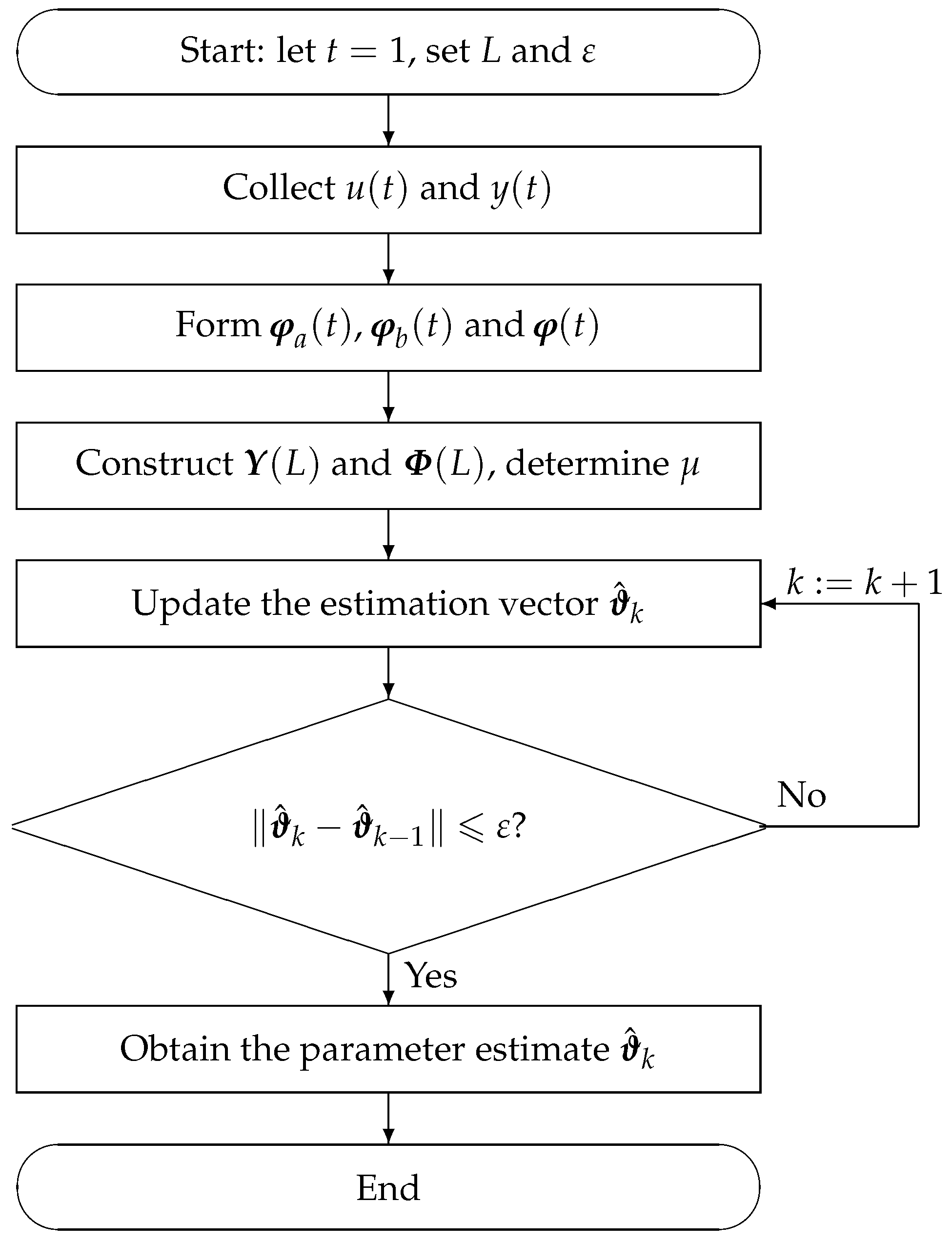
- For , all the variables are set to zero. Let , give the data length L () and set the initial values: , , and the parameter estimation accuracy .
- Collect the input and output data and , , 2, ⋯, L.
- Form the information vectors , and using Equations (8)–(9) and (7).
- Construct the stacked output vector by Equation (5) and the stacked information matrix by Equation (6), select a large according to Equation (4).
- Update the parameter vector estimate using Equation (3).
- Compare with : If , increase k by 1 and go to step 5; otherwise, obtain the iteration k and the parameter estimation vector .
| Algorithm 1 The pseudo-code of implementing the gradient-based iterative algorithm. |
|
4. The Multi-Innovation Gradient-Based Iterative Algorithm
- For , all the variables are set to zero. Let , give the data length p () and set the initial values: , , the maximum iteration and the accuracy .
- Let , collect the input and output data and .
- Form the information vectors , and using Equations (21)–(22) and (20).
- Construct the stacked output vector by Equation (18) and the stacked information matrix by Equation (19), select a large according to Equation (17).
- Update the parameter vector estimate using Equation (16).
- If , increase k by 1 and go to Step 5; otherwise, proceed with the next step.
- Compare with : If , set and increase k by 1 and go to step 2; otherwise, obtain the parameter estimation vector .
5. Example
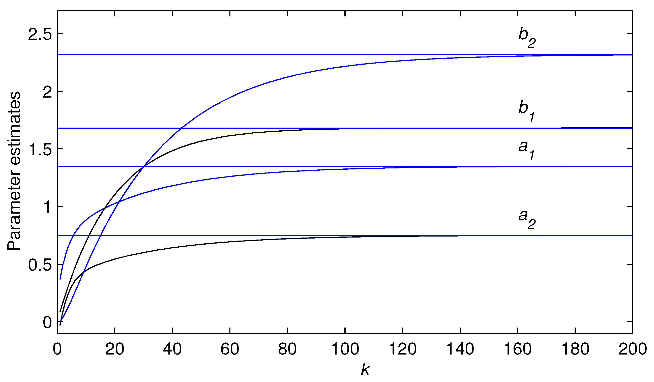
- The GI parameter estimates approach to their true values for sufficiently large data length as the iteration k increases—see Figure 5.
6. Conclusions
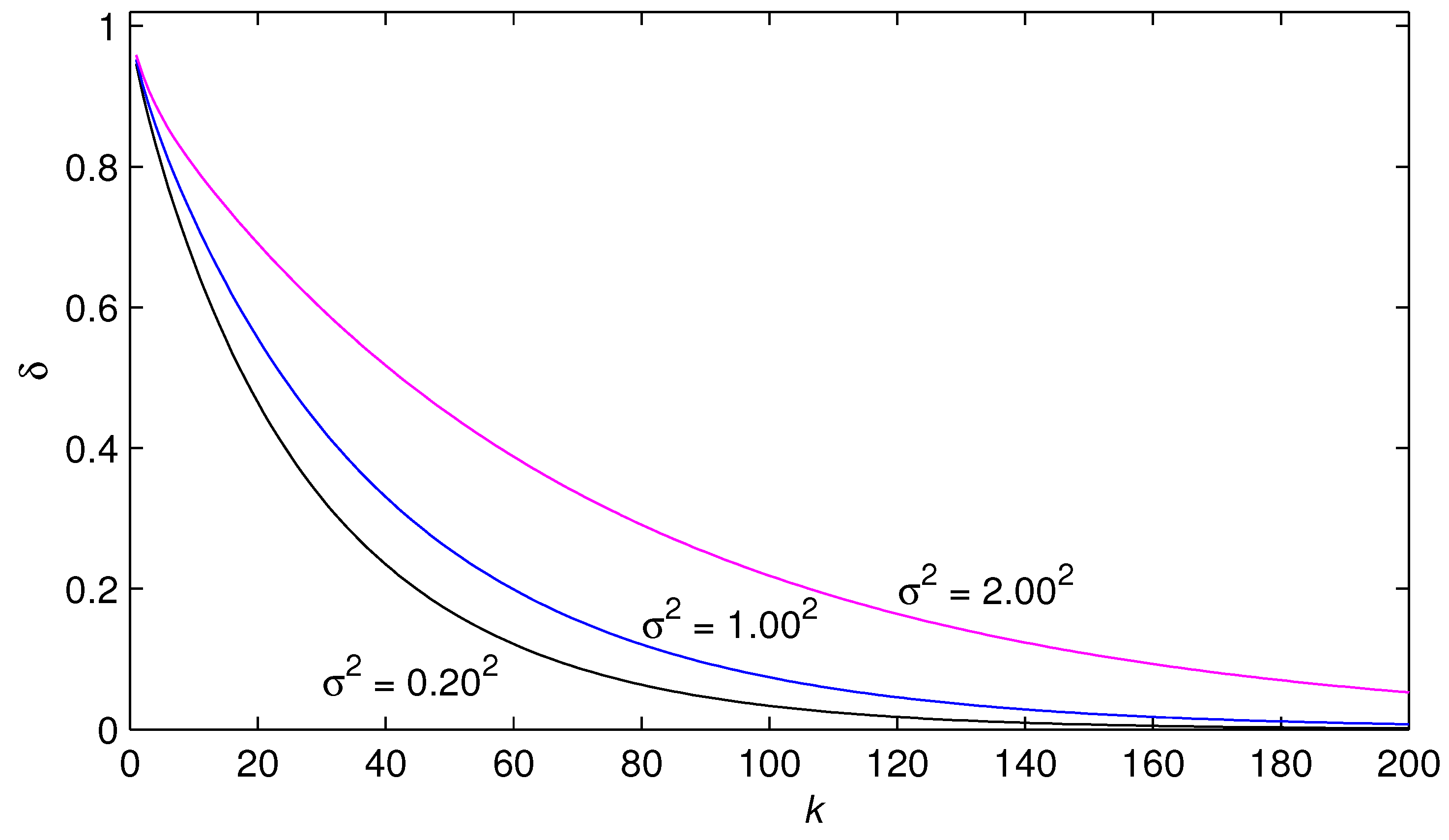
- For a lower noise level, the gradient-based algorithm can give more accurate parameter estimates. The parameter estimation errors become smaller as the iterative index increases.
- The gradient-based iterative parameter estimates approach their true values for sufficiently large data length and iterative index.
- The multi-innovation gradient-based iterative algorithm can track time-varying parameters of dynamical systems, improving the performance of the algorithms.
- The simulation results indicate that the proposed algorithms are effective for estimating the parameters of stochastic systems.
Author Contributions
Funding
Conflicts of Interest
References
- Ding, F. System Identification—New Theory and Methods; Science Press: Beijing, China, 2013; Available online: http://www.bookask.com/book/631454.html (accessed on 5 April 2019). (In Chinese)
- Ding, F. System Identification—Performances Analysis for Identification Methods; Science Press: Beijing, China, 2014; Available online: http://product.dangdang.com/23511899.html?ddclick_reco_product_alsobuy (accessed on 5 April 2019). (In Chinese)
- Ding, F. System Identification—Auxiliary Model Identification Idea and Methods; Science Press: Beijing, China, 2017; Available online: http://www.zxhsd.com/kgsm/ts/2017/07/07/3878821.shtml (accessed on 5 April 2019). (In Chinese)
- Ding, F. System Identification—Iterative Search Principle and Identification Methods; Science Press: Beijing, China, 2018; Available online: https://item.jd.com/12438606.html (accessed on 5 April 2019). (In Chinese)
- Ding, F. System Identification—Multi-Innovation Identification Theory and Methods; Science Press: Beijing, China, 2016; Available online: http://product.dangdang.com/23933240.html (accessed on 5 April 2019). (In Chinese)
- Xu, L. The damping iterative parameter identification method for dynamical systems based on the sine signal measurement. Signal Process. 2016, 120, 660–667. [Google Scholar] [CrossRef]
- Xu, L. A proportional differential control method for a time-delay system using the Taylor expansion approximation. Appl. Math. Comput. 2014, 236, 391–399. [Google Scholar] [CrossRef]
- Xu, L.; Ding, F. Parameter estimation for control systems based on impulse responses. Int. J. Control Autom. Syst. 2017, 15, 2471–2479. [Google Scholar] [CrossRef]
- Li, M.H.; Liu, X.M. The least squares based iterative algorithms for parameter estimation of a bilinear system with autoregressive noise using the data filtering technique. Signal Process. 2018, 147, 23–34. [Google Scholar] [CrossRef]
- Xu, L.; Chen, L.; Xiong, W.L. Parameter estimation and controller design for dynamic systems from the step responses based on the Newton iteration. Nonlinear Dyn. 2015, 79, 2155–2163. [Google Scholar] [CrossRef]
- Xu, L. The parameter estimation algorithms based on the dynamical response measurement data. Adv. Mech. Eng. 2017, 9, 1–12. [Google Scholar] [CrossRef]
- Tian, X.P.; Niu, H.M. A bi-objective model with sequential search algorithm for optimizing network-wide train timetables. Comput. Ind. Eng. 2019, 127, 1259–1272. [Google Scholar] [CrossRef]
- Yang, F.; Zhang, P.; Li, X.X. The truncation method for the Cauchy problem of the inhomogeneous Helmholtz equation. Appl. Anal. 2019, 98, 991–1004. [Google Scholar] [CrossRef]
- Zhao, N.; Liu, R.; Chen, Y.; Wu, M.; Jiang, Y.; Xiong, W.; Liu, C. Contract design for relay incentive mechanism under dual asymmetric information in cooperative networks. Wirel. Netw. 2018, 24, 3029–3044. [Google Scholar] [CrossRef]
- Xu, G.H.; Shekofteh, Y.; Akgul, A.; Li, C.B.; Panahi, S. A new chaotic system with a self-excited attractor: Entropy measurement, signal encryption, and parameter estimation. Entropy 2018, 20, 86. [Google Scholar] [CrossRef]
- Li, X.Y.; Li, H.X.; Wu, B.Y. Piecewise reproducing kernel method for linear impulsive delay differential equations with piecewise constant arguments. Appl. Math. Comput. 2019, 349, 304–313. [Google Scholar] [CrossRef]
- Noshadi, A.; Shi, J.; Lee, W.S.; Shi, P.; Kalam, A. System identification and robust control of multi-input multi-output active magnetic bearing systems. IEEE Trans. Control. Syst. Technol. 2016, 24, 1227–1239. [Google Scholar] [CrossRef]
- Pan, J.; Li, W.; Zhang, H.P. Control algorithms of magnetic suspension systems based on the improved double exponential reaching law of sliding mode control. Int. J. Control Autom. Syst. 2018, 16, 2878–2887. [Google Scholar] [CrossRef]
- Zhang, X.; Ding, F.; Xu, L.; Yang, E.F. Highly computationally efficient state filter based on the delta operator. Int. J. Adapt. Control Signal Process. 2019. [Google Scholar] [CrossRef]
- Luo, X.S.; Song, Y.D. Data-driven predictive control of Hammerstein-Wiener systems based on subspace identification. Inf. Sci. 2018, 422, 447–461. [Google Scholar] [CrossRef]
- Ma, F.Y.; Yin, Y.K.; Li, M. Start-up process modelling of sediment microbial fuel cells based on data driven. Math. Probl. Eng. 2019, 2019, 7403732. [Google Scholar] [CrossRef]
- Li, M.H.; Liu, X.M. Auxiliary model based least squares iterative algorithms for parameter estimation of bilinear systems using interval-varying measurements. IEEE Access 2018, 6, 21518–21529. [Google Scholar] [CrossRef]
- Bottegal, G.; Castro-Garcia, R.; Suykens, J.A.K. A two-experiment approach to Wiener system identification. Automatica 2018, 93, 282–289. [Google Scholar] [CrossRef]
- Guo, F.; Hariprasad, K.; Huang, B.; Ding, Y.S. Robust identification for nonlinear errors-in-variables systems using the EM algorithm. J. Process. Control. 2017, 54, 129–137. [Google Scholar] [CrossRef]
- Li, M.H.; Liu, X.M.; Ding, F. Filtering-based maximum likelihood gradient iterative estimation algorithm for bilinear systems with autoregressive moving average noise. Circuits Syst. Signal Process. 2019, 37, 5023–5048. [Google Scholar] [CrossRef]
- Zhang, X.; Ding, F.; Xu, L.; Yang, E.F. State filtering-based least squares parameter estimation for bilinear systems using the hierarchical identification principle. IET Control Theory Appl. 2018, 12, 1704–1713. [Google Scholar] [CrossRef]
- Ding, F. Two-stage least squares based iterative estimation algorithm for CARARMA system modeling. Appl. Math. Model. 2013, 37, 4798–4808. [Google Scholar] [CrossRef]
- Xu, H.; Ding, F.; Yang, E.F. Modeling a nonlinear process using the exponential autoregressive time series model. Nonlinear Dyn. 2019, 95, 2079–2092. [Google Scholar] [CrossRef]
- Ding, F. Decomposition based fast least squares algorithm for output error systems. Signal Process. 2013, 93, 1235–1242. [Google Scholar] [CrossRef]
- Ge, Z.W.; Ding, F.; Xu, L.; Alsaedi, A.; Hayat, T. Gradient-based iterative identification method for multivariate equation-error autoregressive moving average systems using the decomposition technique. J. Frankl. Inst. 2019, 356, 1658–1676. [Google Scholar] [CrossRef]
- Pan, J.; Ma, H.; Jiang, X.; Ding, W.; Ding, F. Adaptive gradient-based iterative algorithm for multivariate controlled autoregressive moving average systems using the data filtering technique. Complexity 2018, 2018, 9598307. [Google Scholar] [CrossRef]
- Xu, L. Application of the Newton iteration algorithm to the parameter estimation for dynamical systems. J. Comput. Appl. Math. 2015, 288, 33–43. [Google Scholar] [CrossRef]
- Wang, Y.J.; Ding, F. Iterative estimation for a non-linear IIR filter with moving average noise by means of the data filtering technique. IMA J. Math. Control Inf. 2017, 34, 745–764. [Google Scholar] [CrossRef]
- Liu, Y.J.; Wang, D.Q.; Ding, F. Least squares based iterative algorithms for identifying Box-Jenkins models with finite measurement data. Digit. Signal Process. 2010, 20, 1458–1467. [Google Scholar] [CrossRef]
- Liu, Q.Y.; Ding, F. Auxiliary model-based recursive generalized least squares algorithm for multivariate output-error autoregressive systems using the data filtering. Circuits Syst. Signal Process. 2019, 38, 590–610. [Google Scholar] [CrossRef]
- Xu, L.; Ding, F.; Gu, Y.; Alsaedi, A.; Hayat, T. A multi-innovation state and parameter estimation algorithm for a state space system with d-step state-delay. Signal Process. 2017, 140, 97–103. [Google Scholar] [CrossRef]
- Xu, L.; Ding, F. Iterative parameter estimation for signal models based on measured data. Circuits Syst. Signal Process. 2018, 37, 3046–3069. [Google Scholar] [CrossRef]
- Xu, L.; Xiong, W.L.; Alsaedi, A.; Hayat, T. Hierarchical parameter estimation for the frequency response based on the dynamical window data. Int. J. Control Autom. Syst. 2018, 16, 1756–1764. [Google Scholar] [CrossRef]
- Ding, F.; Liu, X.P.; Liu, G. Gradient based and least-squares based iterative identification methods for OE and OEMA systems. Digit. Signal Process. 2010, 20, 664–677. [Google Scholar] [CrossRef]
- Xu, L.; Ding, F. Recursive least squares and multi-innovation stochastic gradient parameter estimation methods for signal modeling. Circuits Syst. Signal Process. 2017, 36, 1735–1753. [Google Scholar] [CrossRef]
- Pan, J.; Jiang, X.; Wan, X.K.; Ding, W. A filtering based multi-innovation extended stochastic gradient algorithm for multivariable control systems. Int. J. Control. Autom. Syst. 2017, 15, 1189–1197. [Google Scholar] [CrossRef]
- Zhang, X.; Xu, L.; Ding, F.; Hayat, T. Combined state and parameter estimation for a bilinear state space system with moving average noise. J. Frankl. Inst. 2018, 355, 3079–3103. [Google Scholar] [CrossRef]
- Zhang, X.; Ding, F.; Alsaadi, F.E.; Hayat, T. Recursive parameter identification of the dynamical models for bilinear state space systems. Nonlinear Dyn. 2017, 89, 2415–2429. [Google Scholar] [CrossRef]
- Bonami, P.; Biegler, L.T.; Conn, A.R.; Cornuéjols, G.; Grossmann, I.E.; Lairde, C.D.; Lee, J.; Lodi, A.; Margot, F.; Sawaya, N.; et al. An algorithmic framework for convex mixed integer nonlinear programs. Discret. Optim. 2008, 5, 186–204. [Google Scholar] [CrossRef]
- Neumaier, A.; Shcherbina, O.; Huyer, W.; Vinkó, T. A comparison of complete global optimization solvers. Math. Program. 2005, 103, 335–356. [Google Scholar] [CrossRef]
- Lastusilta, T.; Bussieck, M.R.; Westerlund, T. An experimental study of the GAMS/AlphaECP MINLP solver. Ind. Eng. Chem. Res. 2009, 48, 7337–7345. [Google Scholar] [CrossRef]
- Klanšek, U. A comparison between MILP and MINLP approaches to optimal solution of nonlinear discrete transportation problem. Transport 2015, 30, 135–144. [Google Scholar] [CrossRef]
- Ding, F.; Liu, X.G.; Chu, J. Gradient-based and least-squares-based iterative algorithms for Hammerstein systems using the hierarchical identification principle. IET Control Theory Appl. 2013, 7, 176–184. [Google Scholar] [CrossRef]
- Xu, L.; Ding, F. Parameter estimation algorithms for dynamical response signals based on the multi-innovation theory and the hierarchical principle. IET Signal Process. 2017, 11, 228–237. [Google Scholar] [CrossRef]
- Wu, M.H.; Li, X.; Liu, C.; Liu, M.; Zhao, N.; Wang, J.; Wan, X.K.; Rao, Z.H.; Zhu, L. Robust global motion estimation for video security based on improved k-means clustering. J. AmbientIntell. Humaniz. Comput. 2019, 10, 439–448. [Google Scholar] [CrossRef]
- Wan, X.K.; Wu, H.; Qiao, F.; Li, F.; Li, Y.; Yan, Y.; Wei, J. Electrocardiogram baseline wander suppression based on the combination of morphological and wavelet transformation based filtering. Computat. Math. Methods Med. 2019, 201, 7196156. [Google Scholar] [CrossRef] [PubMed]
- Wen, Y.Z.; Yin, C.C. Solution of Hamilton-Jacobi-Bellman equation in optimal reinsurance strategy under dynamic VaR constraint. J. Funct. Spaces 2019, 2019, 6750892. [Google Scholar] [CrossRef]
- Yin, C.C.; Zhao, J.S. Nonexponential asymptotics for the solutions of renewal equations, with applications. J. Appl. Probab. 2006, 43, 815–824. [Google Scholar] [CrossRef]
- Yin, C.C.; Wang, C.W. The perturbed compound Poisson risk process with investment and debit interest. Methodol. Comput. Appl. Probab. 2010, 12, 391–413. [Google Scholar] [CrossRef]
- Yin, C.C.; Yuen, K.C. Optimality of the threshold dividend strategy for the compound Poisson model. Stat. Probab. Lett. 2011, 81, 1841–1846. [Google Scholar] [CrossRef]
- Yin, C.C.; Wen, Y.Z. Exit problems for jump processes with applications to dividend problems. J. Comput. Appl. Math. 2013, 245, 30–52. [Google Scholar] [CrossRef]
- Yin, C.C.; Wen, Y.Z. Optimal dividend problem with a terminal value for spectrally positive Levy processes. Insur. Math. Econ. 2013, 53, 769–773. [Google Scholar] [CrossRef]
- Yin, C.C.; Wen, Y.Z.; Zhao, Y.X. On the optimal dividend problem for a spectrally positive levy process. Astin Bull. 2014, 44, 635–651. [Google Scholar] [CrossRef]
- Yin, C.C.; Yuen, K.C. Exact joint laws associated with spectrally negative Levy processes and applications to insurance risk theory. Front. Math. China 2014, 9, 1453–1471. [Google Scholar] [CrossRef]
- Yin, C.C.; Yuen, K.C. Optimal dividend problems for a jump-diffusion model with capital injections and proportional transaction costs. J. Ind. Manag. Optim. 2015, 11, 1247–1262. [Google Scholar] [CrossRef]
- Zhang, X.; Ding, F.; Xu, L.; Alsaedi, A.; Hayat, T. A hierarchical approach for joint parameter and state estimation of a bilinear system with autoregressive noise. Mathematics 2019, 7. [Google Scholar] [CrossRef]
- Xu, L.; Ding, F.; Zhu, Q.M. Hierarchical Newton and least squares iterative estimation algorithm for dynamic systems by transfer functions based on the impulse responses. Int. J. Syst. Sci. 2019, 50, 141–151. [Google Scholar] [CrossRef]
- Wang, Y.J.; Ding, F.; Xu, L. Some new results of designing an IIR filter with colored noise for signal processing. Digit. Signal Process. 2018, 72, 44–58. [Google Scholar] [CrossRef]
- Wang, Y.J.; Ding, F.; Wu, M.H. Recursive parameter estimation algorithm for multivariate output-error systems. J. Frankl. Inst. 2018, 355, 5163–5181. [Google Scholar] [CrossRef]
- Sun, Z.Y.; Zhang, D.; Meng, Q.; Chen, C.C. Feedback stabilization of time-delay nonlinear systems with continuous time-varying output function. Int. J. Syst. Sci. 2019, 50, 244–255. [Google Scholar] [CrossRef]
- Zhan, X.S.; Cheng, L.L.; Wu, J.; Yang, Q.S.; Han, T. Optimal modified performance of MIMO networked control systems with multi-parameter constraints. ISA Trans. 2019, 84, 111–117. [Google Scholar] [CrossRef]
- Zha, X.S.; Guan, Z.H.; Zhang, X.H.; Yuan, F.S. Optimal tracking performance and design of networked control systems with packet dropout. J. Frankl. Inst. 2013, 350, 3205–3216. [Google Scholar]
- Jiang, C.M.; Zhang, F.F.; Li, T.X. Synchronization and antisynchronization of N-coupled fractional-order complex chaotic systems with ring connection. Math. Methods Appl. Sci. 2018, 41, 2625–2638. [Google Scholar] [CrossRef]
- Wang, T.; Liu, L.; Zhang, J.; Schaeffer, E.; Wang, Y. A M-EKF fault detection strategy of insulation system for marine current turbine. Mech. Syst. Signal Process. 2019, 115, 269–280. [Google Scholar] [CrossRef]
- Cao, Y.; Lu, H.; Wen, T. A safety computer system based on multi-sensor data processing. Sensors 2019, 19, 818. [Google Scholar] [CrossRef] [PubMed]
- Cao, Y.; Zhang, Y.; Wen, T.; Li, P. Research on dynamic nonlinear input prediction of fault diagnosis based on fractional differential operator equation in high-speed train control system. Chaos 2019, 29, 013130. [Google Scholar] [CrossRef] [PubMed]
- Cao, Y.; Li, P.; Zhang, Y. Parallel processing algorithm for railway signal fault diagnosis data based on cloud computing. Future Gener. Comput. Syst. 2018, 88, 279–283. [Google Scholar] [CrossRef]
- Cao, Y.; Ma, L.C.; Xiao, S.; Zhang, X.; Xu, W. Standard analysis for transfer delay in CTCS-3. Chin. J. Electron. 2017, 26, 1057–1063. [Google Scholar] [CrossRef]
- Zhao, N.; Wu, M.H.; Chen, J.J. Android-based mobile educational platform for speech signal processing. Int. J. Electr. Eng. Edu. 2017, 54, 3–16. [Google Scholar] [CrossRef]
- Zhao, N.; Chen, Y.; Liu, R.; Wu, M.H.; Xiong, W. Monitoring strategy for relay incentive mechanism in cooperative communication networks. Comput. Electr. Eng. 2017, 60, 14–29. [Google Scholar] [CrossRef]
- Ji, Y.; Ding, F. Multiperiodicity and exponential attractivity of neural networks with mixed delays. Circuits Syst. Signal Process. 2017, 36, 2558–2573. [Google Scholar] [CrossRef]
- Ji, Y.; Liu, X.M. Unified synchronization criteria for hybrid switching-impulsive dynamical networks. Circuits Syst. Signal Process. 2015, 34, 1499–1517. [Google Scholar] [CrossRef]
- Ding, F.; Chen, T. Performance bounds of the forgetting factor least squares algorithm for time-varying systems with finite measurement data. IEEE Trans. Circuits Syst. Regul. Pap. 2005, 52, 555–566. [Google Scholar] [CrossRef]
- Li, N.; Guo, S.; Wang, Y. Weighted preliminary-summation-based principal component analysis for non-Gaussian processes. Control. Eng. Pract. 2019. [Google Scholar] [CrossRef]
- Wang, Y.; Si, Y.; Huang, B.; Lou, Z. Survey on the theoretical research and engineering applications of multivariate statistics process monitoring algorithms: 2008–2017. Can. J. Chem. 2018, 96, 2073–2085. [Google Scholar] [CrossRef]
- Feng, L.; Li, Q.X.; Li, Y.F. Imaging with 3-D aperture synthesis radiometers. IEEE Trans. Geosci. Remote. Sens. 2019, 57, 2395–2406. [Google Scholar] [CrossRef]
- Shi, W.X.; Liu, N.; Zhou, Y.M.; Cao, X.A. Effects of postannealing on the characteristics and reliability of polyfluorene organic light-emitting diodes. IEEE Trans. Electron. Devices 2019, 66, 1057–1062. [Google Scholar] [CrossRef]
- Fu, B.; Ouyang, C.X.; Li, C.S.; Wang, J.W.; Gul, E. An improved mixed integer linear programming approach based on symmetry diminishing for unit commitment of hybrid power system. Energies 2019, 12, 833. [Google Scholar] [CrossRef]
- Wu, T.Z.; Shi, X.; Liao, L.; Zhou, C.J.; Zhou, H.; Su, Y.H. A capacity configuration control strategy to alleviate power fluctuation of hybrid energy storage system based on improved particle swarm optimization. Energies 2019, 12, 642. [Google Scholar] [CrossRef]
- Liu, F.; Xue, Q.; Yabuta, K. Boundedness and continuity of maximal singular integrals and maximal functions on Triebel-Lizorkin spaces. Scie. China-Math. 2019. [Google Scholar] [CrossRef]
- Liu, F. Boundedness and continuity of maximal operators associated to polynomial compound curves on Triebel-Lizorkin spaces. Math. Inequalities Appl. 2019, 22, 25–44. [Google Scholar] [CrossRef]
- Liu, F.; Fu, Z.; Jhang, S. Boundedness and continuity of Marcinkiewicz integrals associated to homogeneous mappings on Triebel-Lizorkin spaces. Front. Math. China 2019, 14, 95–122. [Google Scholar] [CrossRef]
- Ding, J.L. The hierarchical iterative identification algorithm for multi-input-output-error systems with autoregressive noise. Complexity 2017, 2017, 1–11. [Google Scholar] [CrossRef]
- Wang, D.Q.; Yan, Y.R.; Liu, Y.J.; Ding, J.H. Model recovery for Hammerstein systems using the hierarchical orthogonal matching pursuit method. J. Computat. Appl. Math. 2019, 345, 135–145. [Google Scholar] [CrossRef]
- Wang, D.Q.; Li, L.W.; Ji, Y.; Yan, Y.R. Model recovery for Hammerstein systems using the auxiliary model based orthogonal matching pursuit method. Appl. Math. Modell. 2018, 54, 537–550. [Google Scholar] [CrossRef]


| Variables | Expressions | Multiplications | Additions |
|---|---|---|---|
| Sum | |||
| Total flops | |||
| k | |||||
|---|---|---|---|---|---|
| 1 | 0.36787 | −0.03138 | 0.08512 | 0.00447 | 94.61743 |
| 2 | 0.49364 | 0.09219 | 0.16729 | 0.03988 | 90.39550 |
| 5 | 0.72013 | 0.30680 | 0.39043 | 0.18999 | 80.09229 |
| 10 | 0.88253 | 0.44424 | 0.69306 | 0.47742 | 66.48636 |
| 20 | 1.02561 | 0.54320 | 1.10288 | 0.97583 | 46.48051 |
| 50 | 1.22656 | 0.67165 | 1.56551 | 1.80449 | 16.83784 |
| 100 | 1.32469 | 0.73450 | 1.67354 | 2.21545 | 3.34572 |
| 150 | 1.34439 | 0.74715 | 1.68095 | 2.29850 | 0.68915 |
| 200 | 1.34836 | 0.74970 | 1.68146 | 2.31527 | 0.16042 |
| True values | 1.35000 | 0.75000 | 1.68000 | 2.32000 | - |
| k | |||||
|---|---|---|---|---|---|
| 1 | 0.39074 | −0.07246 | 0.05593 | 0.00225 | 95.24273 |
| 2 | 0.51599 | 0.05176 | 0.11093 | 0.02612 | 91.71095 |
| 5 | 0.75720 | 0.28762 | 0.26578 | 0.12989 | 83.37742 |
| 10 | 0.93536 | 0.45376 | 0.49189 | 0.34387 | 72.56593 |
| 20 | 1.05985 | 0.55458 | 0.84302 | 0.75447 | 55.60085 |
| 50 | 1.20990 | 0.65849 | 1.39092 | 1.55649 | 25.60909 |
| 100 | 1.30606 | 0.72444 | 1.63629 | 2.08855 | 7.40476 |
| 150 | 1.33488 | 0.74426 | 1.67889 | 2.24897 | 2.23868 |
| 200 | 1.34356 | 0.75024 | 1.68613 | 2.29741 | 0.74605 |
| True values | 1.35000 | 0.75000 | 1.68000 | 2.32000 | - |
| k | |||||
|---|---|---|---|---|---|
| 1 | 0.41321 | −0.11502 | 0.02712 | 0.00069 | 95.88923 |
| 2 | 0.53665 | 0.00817 | 0.05426 | 0.01247 | 93.10387 |
| 5 | 0.79437 | 0.26457 | 0.13329 | 0.06494 | 87.03542 |
| 10 | 1.00553 | 0.47258 | 0.25709 | 0.18223 | 80.07592 |
| 20 | 1.13655 | 0.59653 | 0.47660 | 0.43831 | 69.11109 |
| 50 | 1.21869 | 0.66123 | 0.95452 | 1.06581 | 44.78973 |
| 100 | 1.28208 | 0.70753 | 1.37278 | 1.68366 | 21.85326 |
| 150 | 1.31416 | 0.73098 | 1.55522 | 1.99714 | 10.70952 |
| 200 | 1.33042 | 0.74288 | 1.63461 | 2.15631 | 5.25922 |
| True values | 1.35000 | 0.75000 | 1.68000 | 2.32000 | - |
© 2019 by the authors. Licensee MDPI, Basel, Switzerland. This article is an open access article distributed under the terms and conditions of the Creative Commons Attribution (CC BY) license (http://creativecommons.org/licenses/by/4.0/).
Share and Cite
Ding, F.; Pan, J.; Alsaedi, A.; Hayat, T. Gradient-Based Iterative Parameter Estimation Algorithms for Dynamical Systems from Observation Data. Mathematics 2019, 7, 428. https://doi.org/10.3390/math7050428
Ding F, Pan J, Alsaedi A, Hayat T. Gradient-Based Iterative Parameter Estimation Algorithms for Dynamical Systems from Observation Data. Mathematics. 2019; 7(5):428. https://doi.org/10.3390/math7050428
Chicago/Turabian StyleDing, Feng, Jian Pan, Ahmed Alsaedi, and Tasawar Hayat. 2019. "Gradient-Based Iterative Parameter Estimation Algorithms for Dynamical Systems from Observation Data" Mathematics 7, no. 5: 428. https://doi.org/10.3390/math7050428
APA StyleDing, F., Pan, J., Alsaedi, A., & Hayat, T. (2019). Gradient-Based Iterative Parameter Estimation Algorithms for Dynamical Systems from Observation Data. Mathematics, 7(5), 428. https://doi.org/10.3390/math7050428


