Retrieving a Context Tree from EEG Data

Abstract

It has been repeatedly conjectured that the brain retrieves statistical regularities from stimuli. Here, we present a new statistical approach allowing to address this conjecture. This approach is based on a new class of stochastic processes, namely, sequences of random objects driven by chains with memory of variable length.

1. Introduction

Consider the following experimental situation. A listener is exposed to a sequence of auditory stimuli, generated by a stochastic chain, while electroencephalographic (EEG) signals are recorded from his scalp. Starting from Von Helmholtz [1], a classical conjecture in neurobiology claims that the listener’s brain automatically identifies statistical regularities in the sequence of stimuli (see, for instance, [2,3]). If this is the case, then a signature of the stochastic chain generating the stimuli should somehow be encoded in the brain activity. The question is whether this signature can be identified in the EEG data recorded during the experiment. The goal of this paper is to discuss a new probabilistic framework in which this conjecture can be formally addressed.

To model the relationship between the random chain of auditory stimuli and the corresponding EEG data, we introduce a new class of stochastic processes. A process in this class has two components. The first one is a stochastic chain taking values in the set of auditory units. The second one is a sequence of functions corresponding to the sequence of EEG chunks recorded during the exposure of the successive auditory stimuli.

We use a stochastic chain with memory of variable length to model the dependence from the past characterizing the sequence of auditory stimuli. Stochastic chains with memory of variable length were introduced by Rissanen [4], as a universal system for data compression. In his seminal paper, Rissanen observed that in many real life stochastic chains the dependence from the past has not a fixed length. Instead, it changes at each step as a function of the past itself. He called a context the smallest final string of past symbols containing all the information required to predict the next symbol. The set of all contexts defines a partition of the past and can be represented by a rooted and labeled oriented tree. For this reason, many authors call stochastic chains with memory of variable length context tree models. We adopt this terminology here. A non-exhaustive list of articles on context tree models, with applications in biology and linguistics, includes [5,6,7,8,9,10,11,12,13].

An interesting point about stochastic chains with memory of variable length with finite context trees is that they are dense in the $\overline{d}$-topology in the class of chains of infinite order with continuous and non-null transition probabilities and summable continuity rates. This result follows easily from Fernández and Galves [14] and Duarte et al. [15]. We refer the reader to these articles for definitions and more details.

Besides modeling the chain of auditory units, we must also model the relationship between the chain of stimuli and the sequence of EEG chunks. To that end, we assume that at each time step a new EEG chunk is chosen according to a probability measure (defined on suitable class of functions) which depends only on the context assigned to the sequence of auditory units generated up to that time. In particular, this implies that to describe the new class of stochastic chains introduced in this paper, we also need to consider a family of probability measures on the set of functions corresponding to the EEG chunks, indexed by the contexts of the context tree characterizing the chain of auditory stimuli.

In this probabilistic framework, the neurobiological question can now be rigorously addressed as follows. Is it possible to retrieve the context tree characterizing the chain of stimuli from the corresponding EEG data? This is a problem of statistical model selection in the class of stochastic processes we have just informally described.

This article is organized as follows. In Section 2, we provide an informal overview of our approach. In Section 3, we introduce the notation, recall what is a context tree model and introduce the new class of sequences of random objects driven by context tree models. A statistical procedure to select, given the data, a member on the class of sequences of random objects driven by context tree models is presented in Section 4. The theoretical result supporting the proposed method, namely Theorem 1, is given in the same section. In Section 5, we conduct a brief simulation study to illustrate the statistical selection procedure presented in Section 4. The proof of Theorem 1 is given in Section 6.

2. Informal Presentation of Our Approach

Volunteers are exposed to sequences of auditory stimuli generated by a context tree models while EEG signals are recorded. The auditory units used as stimuli are strong beats, weak beats or silent units, represented by symbols $2,1$ and 0, respectively.

The way the sequence of auditory units was generated can be informally described as follows. Start with the deterministic sequence

$$2112112112112\dots .$$

Then, replace each weak beat (symbol 1) by a silent unit (symbol 0) with probability $ϵ$ in an independent way.

An example of a sequence produced by this procedure acting on the basic sequence would be

$$2112012112002\dots .$$

In the sequel, this stochastic chain is denoted by the symbols $(X_0,X_1,X_2,\dots )$.

The stochastic chain just described can be generated step by step by an algorithm using only information from the past. We impose to the algorithm the condition that it uses, at each step, the shortest string of past symbols necessary to generate the next symbol.

This algorithm can be described as follows. To generate $X_n$, given the past $X_{n-1},X_{n-2},\dots$, we first look to the last symbol $X_{n-1}$.

• If $X_{n-1}=2$, then

  $$X_n=\left\{\begin{array}{cc}1,\hfill & \mathrm{with} \mathrm{probability}1-ϵ,\hfill \\ 0,\hfill & \mathrm{with} \mathrm{probability}ϵ.\hfill \end{array}\right.$$
• If $X_{n-1}=1$ or $X_{n-1}=0$, then we need to go back one more step,

  ▪

  if $X_{n-2}=2$, then

  $$X_n=\left\{\begin{array}{cc}1,\hfill & \mathrm{with} \mathrm{probability}1-ϵ,\hfill \\ 0,\hfill & \mathrm{with} \mathrm{probability}ϵ;\hfill \end{array}\right.$$

  ▪

  if $X_{n-2}=1$ or $X_{n-2}=0$, then $X_n=2$ with probability 1.

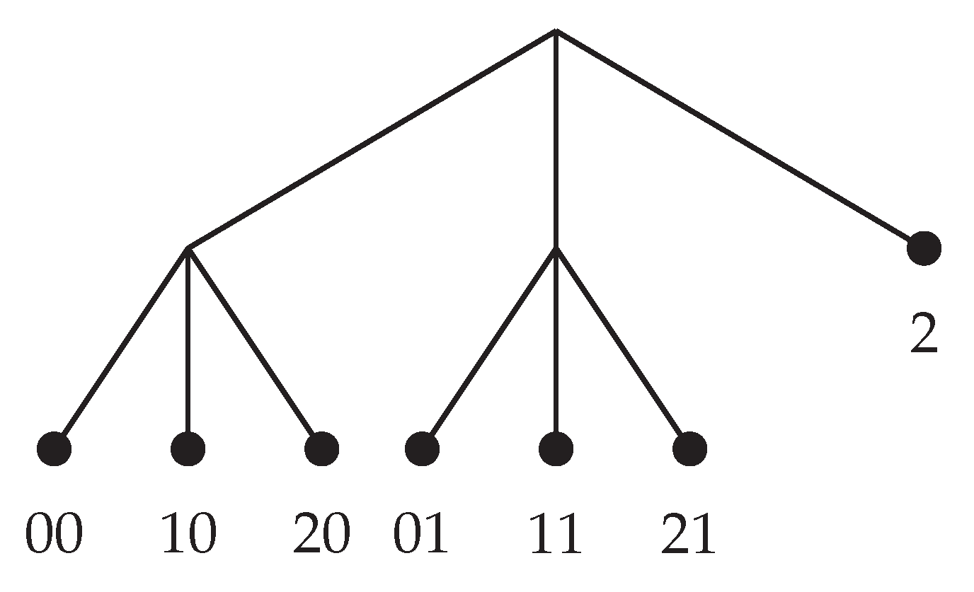
The algorithm described above is characterized by two elements. The first one is a partition of the set of all possible sequences of past units. This partition is represented by the set

$$\tau =\{00,10,20,2,01,11,21,2\}.$$

In partition $\tau$, the string 00 represents the set of all strings ending by the ordered pair $(0,0)$; 10 represents the set of all strings ending by the ordered pair $(1,0)$, …; and finally the symbol 2 represents the set of all strings ending by 2. Following Rissanen [4], let us call context any element of this partition.

For instance, if

$$\dots ,X_{n-3}=1,X_{n-2}=2,X_{n-1}=0,X_n=1.$$

the context associated to this past sequence is 01.

The partition $\tau$ of the past as described above can be represented by a rooted and labeled tree (see Figure 1) where each element of the partition is described as a leaf of the tree.

In the construction described above, for each sequence of past symbols, the algorithm first identifies the corresponding context w in the partition $\tau$. Once the context w is identified, the algorithm chooses a next symbol $a\in \{0,1,2\}$ using the transition probability $p\left(a\right|w)$. In other terms, each context w in $\tau$ defines a probability measure on $\{0,1,2\}$. The family of transition probabilities indexed by elements of the partition is the second element characterizing the algorithm.

The families of transition probabilities associated to $\tau$ are shown in

Table 1. Transition probabilities associated to the context tree $\tau .$

Context w	$\mathbf{p}\left(0\right|\mathbf{w})$	$\mathbf{p}\left(1\right|\mathbf{w})$	$\mathbf{p}\left(2\right|\mathbf{w})$
2	$ϵ$	$1-ϵ$	0
21	$ϵ$	$1-ϵ$	0
20	$ϵ$	$1-ϵ$	0
11	0	0	1
10	0	0	1
01	0	0	1
00	0	0	1

.

Using the notion of context tree, the neurobiological conjecture can now be rephrased as follows. Is the brain able to identify the context tree generating the sample of auditory stimuli? From an experimental point of view, the question is whether it is possible to retrieve the tree presented in Figure 1 from the corresponding EEG data. To deal with this question we introduce a new statistical model selection procedure described below.

Let $Y_n$ be the chunk of EEG data recorded while the volunteer is exposed to the auditory stimulus $X_n$. Observe that $Y_n$ is a continuous function taking values in ${\mathbb{R}}^d$, where $d\ge 1$ is the number of electrodes. Its domain is the time interval of length, say T, during which the acoustic stimulus $X_n$ is presented.

The statistical procedure introduced in the paper can be informally described as follows. Given a sample $(X_0,Y_0),\dots ,(X_n,Y_n)$ of auditory stimuli and associated EEG chunks and for a suitable initial integer $k\ge 1$, do the following.

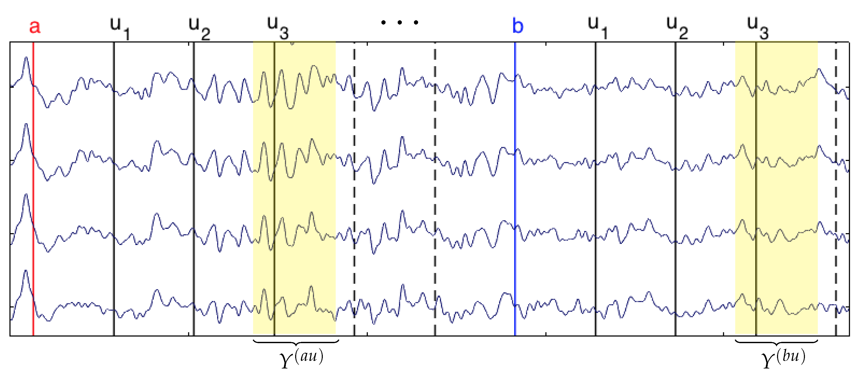
• For each string $\mathbf{u}=u_1,u_2,\dots ,u_k$ of symbols in $\{0,1,2\}$, identify all occurrences in the sequence $X_0,X_1,\dots ,X_n$ of the string $a\mathbf{u}$, obtained by concatenating the symbol $a\in \{0,1,2\}$ and the string $\mathbf{u}$.
• For each $a\in \{0,1,2\}$, define the subsample of all EEG chunks $Y_m=Y_m^{\left(a\mathbf{u}\right)}$ such that $X_{m-k}=a,X_{m-k+1}=u_1,\dots ,X_m=u_k$ (see Figure 2).
• For any pair $a,b\in \{0,1,2\}$, test the null hypothesis that the law of the EEG chunks $Y^{\left(a\mathbf{u}\right)}$ and $Y^{\left(b\mathbf{u}\right)}$ collected at Step 2 are equal.

  (a)

  If the null hypothesis is not rejected for any pair of final symbols a and b, we conclude that the occurrence of a or b before the string $\mathbf{u}$ do not affect the law of EEG chunks. Then, we start again the procedure with the one step shorter sequence $\mathbf{u}=u_2,\dots ,u_k$.

  (b)

  If the null hypothesis is rejected for at least one pair of final symbols a and b, we conclude that the law of EEG chunks depend on the entire string $a\mathbf{u}$ and we stop the pruning procedure.

• We keep pruning the sequence $u_1,\dots ,u_k$ until the null-hypothesis is reject for the first time.
• Call ${\widehat{\tau }}_n$ the tree constituted by the strings which remained after the pruning procedure.

The question is whether ${\widehat{\tau }}_n$ coincides with the context tree $\tau$ generating the sequence of auditory stimuli.

An important technical issue must be clarified at this point, namely, how to test the equality of the laws of two subsamples of EEG chunks. This is done using the projective method informally explained below.

Suppose we have two samples of random functions, each sample composed by independent realizations of some fixed law. To test whether the two samples are generated by the same law, we choose at random a “direction” and project each function in the samples in this direction. This produces two new samples of real numbers. Now, we test whether the samples of the projected real numbers have the same law. Under suitable conditions, a theorem by Cuesta-Albertos et al. [16] ensures that for almost all directions if the test does not reject the null hypothesis that the projected samples have the same law, then the original samples also have the same law.

The arguments informally sketched in this section are formally developed in the subsequent sections.

3. Notation and Definitions

Let A be a finite alphabet. Given two integers $m,n\in \mathbb{Z}$ with $m\le n$, the string $(u_m,\dots ,u_n)$ of symbols in A is often denoted by $u_m^n$; its length is $\ell \left(u_m^n\right)=n-m+1$. The empty string is denoted by ∅ and its length is $\ell (\varnothing )=0$. Fixing two strings u and v of elements of A, we denote by $uv$ the string in $A^{\ell \left(u\right)+\ell \left(v\right)}$ obtained by the concatenation of u and v. By definition $u\varnothing =\varnothing u=u$ for any string $u\in A^{\ell \left(u\right)}$. The string u is said to be a suffix of v if there exists a string s satisfying $v=su$. This relation is denoted by $u⪯v$. When $v\ne u$, we say that u is a proper suffix of v and write $u\prec v$. Hereafter, the set of all finite strings of symbols in A is denoted by $A^{\ast }:={\bigcup }_{k=1}^{\infty }{A}^k$. For any finite string $w=w_{-k}^{-1}$ with $k\ge 2$, we write $suf\left(w\right)$ to denote the one-step shorter string $w_{-k+1}^{-1}$.

Definition 1.

A finite subset τ of $A^{\ast }$ is a context tree if it satisfies the following conditions:

1. 

Suffix Property. For no $w\in \tau$ we have $u\in \tau$ with $u\prec w$.

2. 

Irreducibility. No string belonging to τ can be replaced by a proper suffix without violating the suffix property.

The set $\tau$ can be identified with the set of leaves of a rooted tree with a finite set of labeled branches. The elements of $\tau$ are always denoted by $w,u,v,\dots$.

The height of the context tree $\tau$ is defined as $\ell \left(\tau \right)=max\{\ell (w):w\in \tau \}.$ In the present paper, we only consider context trees with finite height.

Definition 2.

Let τ and ${\tau }^{\prime }$ be two context trees. We say that τ is smaller than ${\tau }^{\prime }$ and write $\tau ⪯{\tau }^{\prime }$, if for every $w^{\prime }\in {\tau }^{\prime }$ there exists $w\in \tau$ such that $w⪯w^{\prime }$.

Given a context tree $\tau$, let $p=\left\{p\right(·\mid w):w\in \tau \}$ be a family of probability measures on A indexed by the elements of $\tau$. The pair $(\tau ,p)$ is called a probabilistic context tree on A. Each element of $\tau$ is called a context. For any string $x_{-n}^{-1}\in A^n$ with $n\ge \ell \left(\tau \right)$, we write $c_{\tau }\left(x_{-n}^{-1}\right)$ to denote the only context in $\tau$ which is a suffix of $x_{-n}^{-1}$.

Definition 3.

A probabilistic context tree $(\tau ,p)$ with height $\ell \left(\tau \right)=k$ is irreducible if for any $a_{-k}^{-1}\in A^k$ and $b\in A$ there exist a positive integer $n=n(a_{-k}^{-1},b)$ and symbols $a_0,a_1,\dots ,a_n=b\in A$ such that

$$p\left(a_0\right|c_{\tau }\left(a_{-k}^{-1}\right))>0,p\left(a_1\right|c_{\tau }\left(a_0{a}_{-k}^{-1}\right))>0,\dots ,p\left(a_n\right|c_{\tau }(a_{n-1},\dots ,a_0{a}_{-k}^{-1}))>0.$$

Definition 4.

Let $(\tau ,p)$ be a probabilistic context tree on A. A stochastic chain ${\left(X_n\right)}_{n\in \mathbb{N}}$ taking values in A is called a context tree model compatible with $(\tau ,p)$ if

1. 

for any $n\ge \ell \left(\tau \right)$ and any finite string $x_{-n}^{-1}\in A^n$ such that $P\left(X_0^{n-1}=x_{-n}^{-1}\right)>0$, it holds that

$$P\left(X_n=a\mid X_0^{n-1}=x_{-n}^{-1}\right)=p\left(a\mid c_{\tau }\left(x_{-n}^{-1}\right)\right)foralla\in A,$$

(1)

where $c_{\tau }\left(x_{-n}^{-1}\right)$ is the only context in τ which is a suffix of $x_{-n}^{-1}$.

2. 

For any $1\le j<\ell \left(c_{\tau }\left(x_{-n}^{-1}\right)\right)$, there exists $a\in A$ such that

$$P\left(X_n=a\mid X_0^{n-1}=x_{-n}^{-1}\right)\ne P\left(X_n=a\mid X_{n-j}^{n-1}=x_{-j}^{-1}\right).$$

With this notation, we can now introduce the class of random objects driven by a context tree model.

Definition 5.

Let A be a finite alphabet, $(\tau ,p)$ a probabilistic context tree on A, $(F,\mathcal{F})$ a measurable space and $(Q^w:w\in \tau )$ a family of probability measures on $(F,\mathcal{F})$. The bivariate stochastic chain ${(X_n,Y_n)}_{n\in \mathbb{N}}$ taking values in $A\times F$ is a sequence of random objects driven by a context tree model compatible with $(\tau ,p)$ and $(Q^w:w\in \tau )$ if the following conditions are satisfied:

1. 

${\left(X_n\right)}_{n\in \mathbb{N}}$ is a context tree model compatible with $(\tau ,p)$.

2. 

The random elements $Y_0,Y_1,\dots$ are $\mathcal{F}$-measurable. Moreover, for any integers $\ell \left(\tau \right)\le m\le n$, any string $x_{m-\ell \left(\tau \right)+1}^n\in A^{n-m+\ell \left(\tau \right)}$ and any sequence $J_m,\dots ,J_n$ of $\mathcal{F}$-measurable sets,

$$P\left(Y_m\in J_m,\dots ,Y_n\in J_n|X_{m-\ell \left(\tau \right)+1}^n=x_{m-\ell \left(\tau \right)+1}^n\right)=\prod _{k=m}^n{Q}^{c_{\tau }\left(x_{k-\ell \left(\tau \right)+1}^k\right)}\left(J_k\right),$$

where $c_{\tau }\left(x_{k-\ell \left(\tau \right)+1}^k\right)$ is the context in τ assigned to the string of symbols $x_{k-\ell \left(\tau \right)+1}^k$.

Definition 6.

A sequence of random objects driven by a context tree model compatible with $(\tau ,p)$ and $(Q^w:w\in \tau )$ is identifiable if for any context $w\in \tau$ there exists a context $u\in \tau$ such that suf$\left(w\right)$ = suf$\left(u\right)$ and $Q^w\ne Q^u.$

The process $\left(X_n\right)$ is called the stimulus chain and $\left(Y_n\right)$ is called the response chain.

The experimental situation described in Section 2 can now be formally presented as follows.

• The stimulus chain $\left(X_n\right)$ is a context tree model taking values in an alphabet having as elements symbols indicating the different types of auditory units appearing in the sequence of stimuli. We call $(\tau ,p)$ its probabilistic context tree.
• Each element $Y_n$ of the response chain $\left(Y_n\right)$ represents the EEG chunk recorded while the volunteer is exposed to the auditory stimulus $X_n$. Thus, $Y_n=(Y_n\left(t\right),t\in [0,T])$ is a function taking values in ${\mathbb{R}}^d$, where T is the time distance between the onsets of two consecutive auditory stimuli and d the number of electrodes used in the analysis. The sample space F is the Hilbert space $L^2([0,T],{\mathbb{R}}^d)$ of ${\mathbb{R}}^d$-valued functions on $[0,T]$ having square integrable components. The Hilbert space F is endowed with its usual Borel $\sigma$-algebra $\mathcal{F}$.
• Finally, $(Q^w,w\in \tau )$ is a family of probability measures on $L^2([0,T],{\mathbb{R}}^d)$ describing the laws of the EEG chunks.

From now on, the pair $(F,\mathcal{F})$ always denotes the Hilbert space $L^2([0,T],{\mathbb{R}}^d)$ endowed with its usual Borel $\sigma$-algebra.

4. Statistical Selection for Sequences of Random Objects Driven by Context Tree Models

Let $(X_0,Y_0),\dots ,(X_n,Y_n)$, with $X_k\in A$ and $Y_k\in F$ for $0\le k\le n$, be a sample produced by a sequence of random objects driven by a context tree model compatible with $(\overline{\tau },\overline{p})$ and $({\overline{Q}}^w:w\in \overline{\tau })$. Before introducing the statistical selection procedure, we need two more definitions.

Definition 7.

Let τ be a context tree and fix a finite string $s\in A^{\ast }$. We define the branch in τ induced by s as the set $B_{\tau }\left(s\right)=\{w\in \tau :w\succ s\}$. The set $B_{\tau }\left(s\right)$ is called a terminal branch if for all $w\in B_{\tau }\left(s\right)$ it holds that $w=as$ for some $a\in A$.

Given a sample $X_0,\dots ,X_n$ of symbols in A and a finite string $u\in A^{\ast }$, the number of occurrences of u in the sample $X_0,\dots ,X_n$ is defined as

$$N_n\left(u\right)=\sum _{m=l\left(u\right)-1}^{n}1\{X_{m-\ell \left(u\right)+1}^m=u\}.$$

Definition 8.

Given integers $n>L\ge 1$, an admissible context tree of maximal height L for the sample $X_0,\dots ,X_n$ of symbols in A, is any context tree τ satisfying

1. 

$w\in \tau$ if and only if $\ell \left(w\right)\le L$ and $N_n\left(w\right)\ge 1$.

2. 

Any string $u\in A^{\ast }$ with $N_n\left(u\right)\ge 1$ is a suffix of some $w\in \tau$ or has a suffix $w\in \tau$.

For any pair of integers $1\le L<n$ and any string $u\in A^{\ast }$ with $\ell \left(u\right)\le L$, call $I_n\left(u\right)$ the set of indexes belonging to $\{\ell (u)-1,\dots ,n\}$ in which the string u appears in sample $X_0,\dots ,X_n$, that is

$$I_n\left(u\right)=\{\ell \left(u\right)-1\le m\le n:X_{m-\ell \left(u\right)+1}^m=u\}.$$

Observe that by definition $|I_n\left(u\right)|=N_n\left(u\right)$. If $I_n\left(u\right)=\{m_1,\dots ,m_{N_n\left(u\right)}\}$, we set $Y_k^{\left(u\right)}=Y_{m_k}$ for each $1\le k\le N_n\left(u\right)$. Thus, $Y_1^{\left(u\right)},\dots ,Y_{N_n\left(u\right)}^{\left(u\right)}$ is the subsample of $Y_0,\dots ,Y_n$ induced by the string u.

Given $u\in A^{\ast }$ such that $N_n\left(u\right)\ge 1$ and $h\in F$, we define the empirical distribution associated to the projection of the sample $Y_1^{\left(u\right)},\dots ,Y_{N_n\left(u\right)}^{\left(u\right)}$ onto the direction h as

$${\widehat{Q}}_n^{u,h}\left(t\right)=\frac{1}{N_n\left(u\right)}\sum _{m=1}^{N_n\left(u\right)}{1}_{(-\infty ,t]}\left(\langle Y_m^{\left(u\right)},h\rangle \right),t\in \mathbb{R},$$

where for any pair of functions $f,h\in F$,

$$\langle f,h\rangle =\sum _{i=1}^d{\int }_0^T{f}_i\left(t\right)h_i\left(t\right)dt.$$

For a given pair $u,v\in A^{\ast }$, with $max\{\ell (u),\ell (v\left)\right\}\le L$ and $h\in F$, the Kolmogorov–Smirnov distance between the empirical distributions ${\widehat{Q}}_n^{u,h}$ and ${\widehat{Q}}_n^{v,h}$ is defined by

$$\mathrm{KS}({\widehat{Q}}_n^{u,h},{\widehat{Q}}_n^{v,h})=\underset{t\in \mathbb{R}}{sup}|{\widehat{Q}}_n^{u,h}\left(t\right)-{\widehat{Q}}_n^{v,h}\left(t\right)|.$$

Finally, we define for any pair $u,v\in A^{\ast }$ such that $max\{\ell (u),\ell (v\left)\right\}\le L$ and $h\in F,$

$$D_n^h((Y_1^{\left(u\right)},\dots ,Y_{N_n\left(u\right)}^{\left(u\right)}),(Y_1^{\left(v\right)},\dots ,Y_{N_n\left(v\right)}^{\left(v\right)}))=\sqrt{\frac{N_n\left(u\right)N_n\left(v\right)}{N_n\left(u\right)+N_n\left(v\right)}}\mathrm{KS}({\widehat{Q}}_n^{u,h},{\widehat{Q}}_n^{v,h}).$$

Our selection procedure can now be described as follows. Fix an integer $1\le L<n$ and let ${\mathcal{T}}_n$ be the largest admissible context tree of maximal height L for the sample $X_0,\dots ,X_n$. The largest means that if $\tau$ is any other admissible context tree of maximal height L for the sample $X_1^n$, then $\tau ⪯{\mathcal{T}}_n.$

For any string $u\in A^{\ast }$ such that $B_{{\mathcal{T}}_n}\left(u\right)$ is a terminal branch, we test the null hypothesis

$$H_0^{\left(u\right)}:\mathcal{L}\left(Y_1^{\left(au\right)},\dots ,Y_{N_n\left(au\right)}^{\left(au\right)}\right)=\mathcal{L}\left(Y_1^{\left(bu\right)},\dots ,Y_{N_n\left(bu\right)}^{\left(bu\right)}\right),\forall au,bu\in B_{{\mathcal{T}}_n}\left(u\right)$$

(2)

using the test statistic

$${∆}_n\left(u\right)={∆}_n^W\left(u\right)=\underset{a,b\in A}{max}{D}_n^W\left((Y_1^{\left(au\right)},\dots ,Y_{N_n\left(au\right)}^{\left(au\right)}),(Y_1^{\left(bu\right)},\dots ,Y_{N_n\left(bu\right)}^{\left(bu\right)})\right),$$

(3)

where $W=((W_1\left(t\right),\dots ,W_d\left(t\right)):t\in [0,T])$ is a realization of a d-dimensional Brownian motion in $[0,T]$.

We reject the null hypothesis $H_0^{\left(u\right)}$ when ${∆}_n\left(u\right)>c$, where $c>0$ is a suitable threshold. When the null hypothesis $H_0^{\left(u\right)}$ is not rejected, we prune the branch $B_{{\mathcal{T}}_n}\left(u\right)$ in ${\mathcal{T}}_n$ and set as a new candidate context tree

$${\mathcal{T}}_n=\left({\mathcal{T}}_n\backslash B_{{\mathcal{T}}_n}\left(u\right)\right)\cup \left\{u\right\}.$$

On the other hand, if the null hypothesis $H_0^{\left(u\right)}$ is rejected, we keep $B_{{\mathcal{T}}_n}\left(u\right)$ in ${\mathcal{T}}_n$ and stop testing $H_0^{\left(s\right)}$ for strings $s\in A^{\ast }$ such that $s⪯u$.

In each pruning step, take a string $s\in A^{\ast }$ that induces a terminal branch in ${\mathcal{T}}_n$ and has not been tested yet. This pruning procedure is repeated until no more pruning is performed. We denote by ${\widehat{\tau }}_n$ the final context tree obtained by this procedure. The formal description of the above pruning procedure is provided in Algorithm 1 as pseudocode.

Algorithm 1 Pseudocode describing the pruning procedure used to select the tree ${\widehat{\tau }}_n$.

Input:  A sample $(X_0,Y_0),\dots ,(X_n,Y_n)$ with $X_k\in A$ and $Y_k\in F$ for $0\le k\le n$, a positive threshold c and a positive integer L. Output:  A tree ${\widehat{\tau }}_n$ 1: $\tau \leftarrow {\mathcal{T}}_n$ 2: Flag$\left(s\right)\leftarrow$ “not visited” for all string s such that $s⪯w\in {\mathcal{T}}_n$ 3: for k in L to 1 do 4:  while $\exists s\in \tau$: $\ell \left(s\right)=k$, Flag$\left(s\right)=$ “not visited” and $B_{\tau }\left(s\right)$ is a terminal branch do 5:   Choose a s such that $\ell \left(s\right)=k$, Flag$\left(s\right)=$ “not visited” and $B_{\tau }\left(s\right)$ is a terminal branch 6:   Compute the test statistic ${∆}_n\left(s\right)$ to test $H_0^{\left(s\right)}$ 7:   if ${∆}_n\left(s\right)>c$ then 8:    Flag$\left(u\right)\leftarrow$ “visited” $\forall u⪯s$ 9:   else 10:    $\tau \leftarrow (\tau \backslash B_{\tau }\left(s\right))\cup \left\{s\right\}$ 11:   end if 12:  end while 13: end for 14: Return${\widehat{\tau }}_n=\tau .$

To state the consistency theorem, we need the following definitions.

Definition 9.

A probability measure P defined on $(F,\mathcal{F})$ satisfies Carleman condition if all the absolute moments $m_k={\int \left|\right|h\left|\right|}^{k}P\left(dh\right)$, $k\ge 1,$ are finite and

$$\sum _{k\ge 1}{m}_k^{-1/k}=+\infty .$$

Definition 10.

Let P be a probability measure on $(F,\mathcal{F})$. We say that P is continuous if $P^h$ is continuous for any $h\in F$, where $P^h$ is defined by

$$P^h\left((-\infty ,t]\right)=P(x\in F:\langle x,h\rangle \le t),t\in \mathbb{R}.$$

Let V be a finite set of indexes and $(P_i:i\in V)$ be a family of probability measures on $(F,\mathcal{F})$. We say that $(P_i:i\in V)$ is continuous if for all $i\in V$, the probability measure $P_i$ is continuous.

In what follows, let $c_{\alpha }=\sqrt{(1/2)ln(2/\alpha )}$, where $\alpha \in (0,1).$ We say that ${\alpha }_n\to 0$ slowly enough as $n\to \infty$ if

$$\frac{\sqrt{n}}{c_{{\alpha }_n}}\to \infty \mathrm{as}n\to \infty .$$

Theorem 1.

Let $(X_0,Y_0),\dots ,(X_n,Y_n)$ be a sample produced by a identifiable sequence of random objects driven by a context tree model compatible with $(\overline{\tau },\overline{p})$ and $({\overline{Q}}_w:w\in \overline{\tau })$, and let ${\widehat{\tau }}_n$ be the context tree selected from the sample by Algorithm 1 with $L\ge \ell \left(\overline{\tau }\right)$ and threshold $c_{{\alpha }_n}=\sqrt{(1/2)ln(2/{\alpha }_n)}$, where ${\alpha }_n\in (0,1)$. If $(\overline{\tau },\overline{p})$ is irreducible and $({\overline{Q}}_w:w\in \overline{\tau })$ is continuous and satisfies Carleman condition, then for ${\alpha }_n\to 0$ slowly enough as $n\to \infty$,

$$\underset{n\to \infty }{lim}P({\widehat{\tau }}_n\ne \overline{\tau })=0.$$

The proof of Theorem 1 is presented in Section 6.

5. Simulation Study

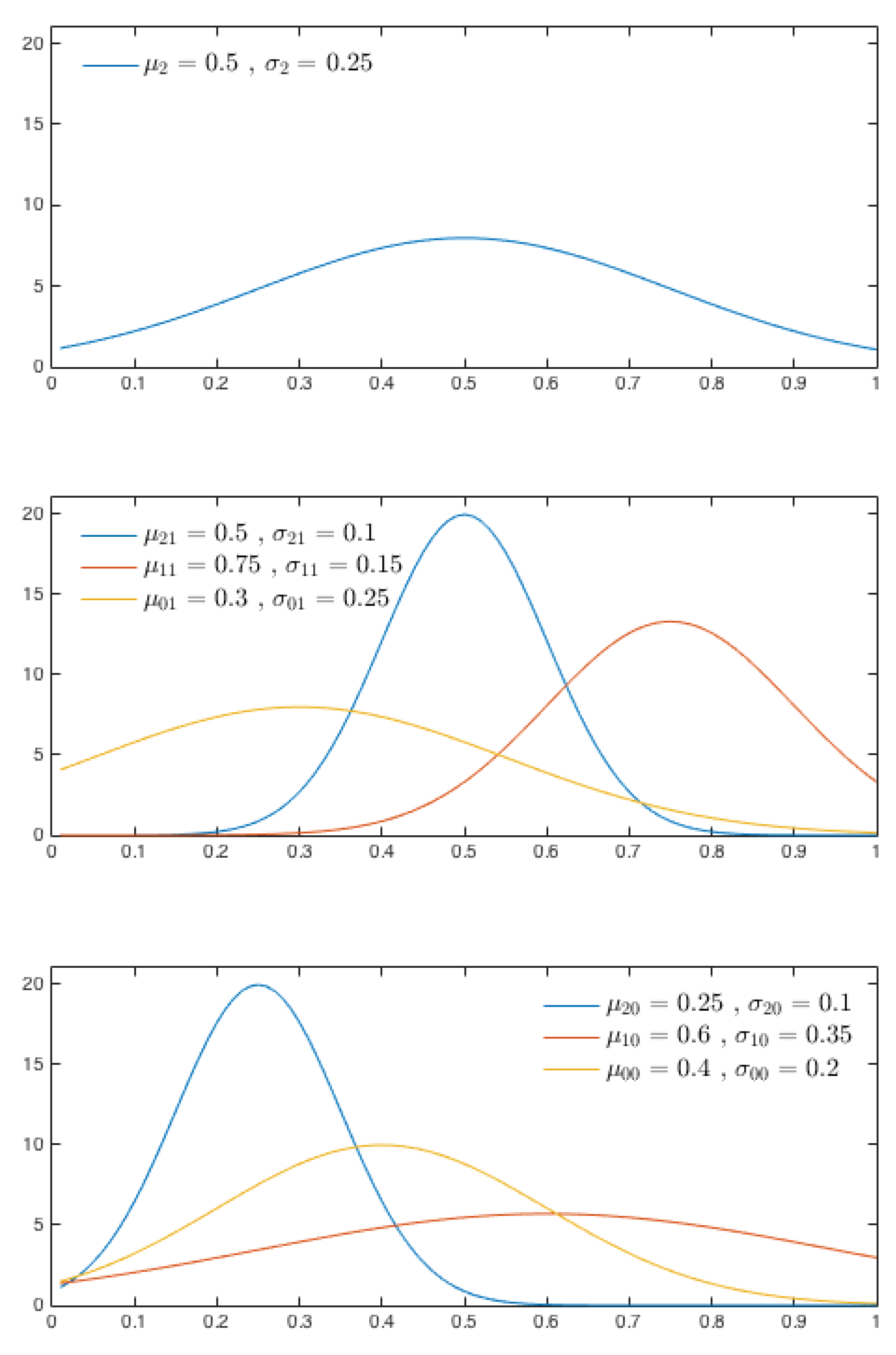
In this section, we illustrate the performance of Algorithm 1 by applying it in a toy example. We consider the context tree model compatible with $(\overline{\tau },\overline{p})$ described in Section 2 with $ϵ=0.2$. For each $w\in \overline{\tau }$, we assume ${\overline{Q}}^w$ is the law of a diffusion process with drift coefficient $f_w={\left(f_w\left(t\right)\right)}_{0\le t\le 1}$ and constant diffusion coefficient. For simplicity, all diffusion coefficients are assumed to be 1. For each context $w\in \overline{\tau }$, we assume $f_w=K{g}_w$, where K is a positive constant and $g_w$ is the density of a Gaussian random variable with mean ${\mu }_w$ and standard deviation ${\sigma }_w$, restricted to the interval $[0,1]$. In the simulation, we take $K=5$. The shapes of the functions $f_w$ and corresponding values of ${\mu }_w$ and ${\sigma }_w$ are shown in Figure 3. One can check that the assumptions of Theorem 1 are satisfied by this toy example.

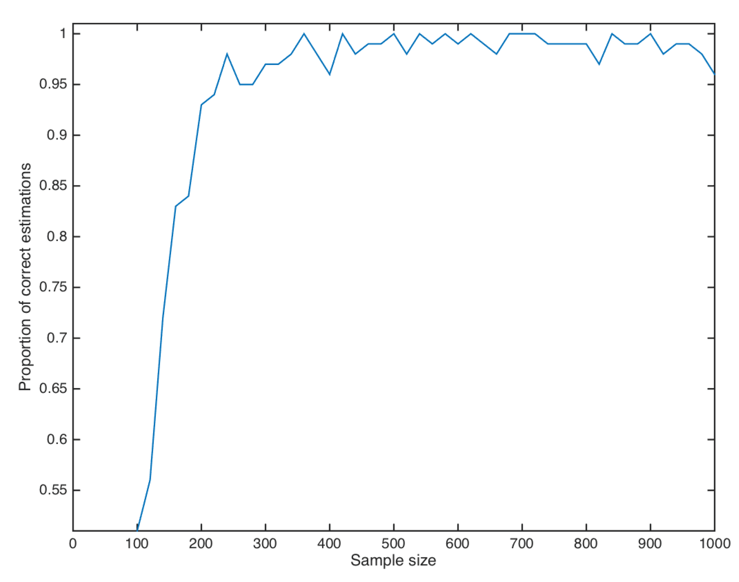
To numerically implement Algorithm 1, we assume that all trajectories of the diffusion processes are observed on equally spaces point $0=t_0<t_1<\dots <t_{100}=1$, where $t_i=\frac{i}{100}$ for each $1\le i\le 100$. For each sample size $n=100,120,140,\dots ,1000,$ we estimate the fraction of times Algorithm 1, with ${\alpha }_n=1/n$ and $L=4$, correctly identifies the context tree $\overline{\tau }$ based on 100 random samples of the model with size $n.$ The results are reported in Figure 4.

6. Proof of Theorem 1

The proof of Theorem 1 is a direct consequence of Propositions 1 and 2 presented below.

Proposition 1.

Let $(X_0,Y_0),\dots ,(X_n,Y_n)$ be a sample produced by a sequence of random objects driven by a context tree model compatible with $(\overline{\tau },\overline{p})$ and $({\overline{Q}}_w:w\in \overline{\tau })$ satisfying the assumptions of Theorem 1. Let $\alpha \in (0,1)$ and set $c_{\alpha }=\sqrt{1/2ln(2/\alpha )}$. For any integer $L\ge \ell \left(\overline{\tau }\right)$, context $w\in \overline{\tau }$, direction $h\in F\backslash \left\{0\right\}$, and strings $u,v\in {\cup }_{k=1}^{L-\ell \left(w\right)}{A}^k$ such that $w⪯u$ and $w⪯v$, it holds that

$$\underset{n\to \infty }{lim}P(D_n^h((Y_1^{\left(u\right)},\dots ,Y_{N_n\left(u\right)}^{\left(u\right)}),(Y_1^{\left(v\right)},\dots ,Y_{N_n\left(v\right)}^{\left(v\right)}))>c_{\alpha })=\alpha .$$

In particular, for any ${\alpha }_n\to 0$ as $n\to \infty$, we have

$$\underset{n\to \infty }{lim}P(D_n^h((Y_1^{\left(u\right)},\dots ,Y_{N_n\left(u\right)}^{\left(u\right)}),(Y_1^{\left(v\right)},\dots ,Y_{N_n\left(v\right)}^{\left(v\right)}))>c_{{\alpha }_n})=0.$$

Proof. 

The irreducibility of $(\overline{\tau },\overline{p})$ implies that P-a.s. both $N_n\left(u\right)$ and $N_n\left(v\right)$ tend to $+\infty$ as n diverges. Thus, Theorem 3.1(a) of [16] implies that the law of $D_n^h((Y_1^{\left(u\right)},\dots ,Y_{N_n\left(u\right)}^{\left(u\right)}),(Y_1^{\left(v\right)},\dots ,Y_{N_n\left(v\right)}^{\left(v\right)}))$ is independent of the strings u and v, and also of the direction $h\in F\backslash \left\{0\right\}$. It also implies that $D_n^h((Y_1^{\left(u\right)},\dots ,Y_{N_n\left(u\right)}^{\left(u\right)}),(Y_1^{\left(v\right)},\dots ,Y_{N_n\left(v\right)}^{\left(v\right)})$ converges in distribution to $K={sup}_{t\in [0,1]}\left|B\left(t\right)\right|$ as $n\to \infty$, where $B=\left(B\right(t):t\in [0,1\left]\right)$ is a Brownian Bridge. Since $P(K>c_{\alpha })=\alpha$, the first part of the result follows.

By the first part of the proof, for any fixed $\alpha \in (0,1)$, we have that for all n large enough,

$$P(D_n^h((Y_1^{\left(u\right)},\dots ,Y_{N_n\left(u\right)}^{\left(u\right)}),(Y_1^{\left(v\right)},\dots ,Y_{N_n\left(v\right)}^{\left(v\right)}))>c_{\alpha }))\le 2\alpha .$$

Thus, given $ϵ>0$, take $\alpha \in (0,1)$ such that $2\alpha <ϵ$ to deduce that for all n large enough,

$$P(D_n^h((Y_1^{\left(u\right)},\dots ,Y_{N_n\left(u\right)}^{\left(u\right)}),(Y_1^{\left(v\right)},\dots ,Y_{N_n\left(v\right)}^{\left(v\right)}))>c_{\alpha }))<ϵ.$$

Since $c_{{\alpha }_n}\to \infty$ as $n\to \infty$, we have that for all n sufficiently large $c_{{\alpha }_n}>c_{\alpha }$ so that the result follows from the previous inequality. □

Proposition 2 reads as follows.

Proposition 2.

Let $(X_0,Y_0),\dots ,(X_n,Y_n)$ be a sample produced by a identifiable sequence of random objects driven by a context tree model compatible with $(\overline{\tau },\overline{p})$ and $({\overline{Q}}_w:w\in \overline{\tau })$, and let ${\widehat{\tau }}_n$ satisfying the assumptions of Theorem 1. Let $\alpha \in (0,1)$ and define $c_{\alpha }=\sqrt{1/2ln(2/\alpha )}$. For any string $s\in A^{\ast }$ such that $B_{\overline{\tau }}\left(s\right)$ is a terminal branch there exists a pair $w,w^{\prime }\in B_{\overline{\tau }}\left(s\right)$ such that for almost all realization of a Brownian motion $W=\left(W\right(t):t\in [0,T\left]\right)$ on $[0,T]$,

$$\underset{n\to \infty }{lim}P(D_n^W((Y_1^{\left(w\right)},\dots ,Y_{N_n\left(w\right)}^{\left(w\right)}),(Y_1^{\left(w^{\prime }\right)},\dots ,Y_{N_n\left(w^{\prime }\right)}^{\left(w^{\prime }\right)}))\le c_{{\alpha }_n})=0,$$

whenever ${\alpha }_n\to 0$ slowly enough as $n\to \infty .$

Proof. 

Since the sequence of random objects $(X_0,Y_0),(X_1,Y_1),\dots$ is identifiable and $B_{\overline{\tau }}\left(s\right)$ is a terminal branch, there exists a pair $w,w^{\prime }\in B_{\overline{\tau }}\left(suf\left(w\right)\right)$ whose associated distributions ${\overline{Q}}^w$ and ${\overline{Q}}^w$ on F are different, and both ${\overline{Q}}^w$ and ${\overline{Q}}^{w^{\prime }}$ satisfy the Carleman condition. For each $n\ge 1$, define

$$N_n:=\sqrt{\frac{N_n\left(w\right)N_n\left(w^{\prime }\right)}{N_n\left(w\right)+N_n\left(w^{\prime }\right)}},$$

if $min\{N_n\left(w\right),N_n\left(w^{\prime }\right)\}\ge 1$. Otherwise, we set $N_n=0$. The irreducibility of $(\overline{\tau },\overline{p})$ implies that $n^{-1/2}{N}_n\to C$ as $n\to \infty$ P-a.s., where C is a positive constant depending on w and $w^{\prime }$.

Now, Theorem 3.1(b) of [16] implies that, for almost all realization of a Brownian motion W on F,

$$\underset{n\to \infty }{\text{lim inf}}\mathrm{KS}({\widehat{Q}}_n^{W,w},{\widehat{Q}}_n^{W,w^{\prime }})>0\mathit{\text{P-}}\mathrm{a}.\mathrm{s}.$$

(4)

Since $D^W((Y_1^{\left(w\right)},\dots ,Y_{N_n\left(w\right)}^{\left(w\right)}),(Y_1^{\left(w^{\prime }\right)},\dots ,Y_{N_n\left(w^{\prime }\right)}^{\left(w^{\prime }\right)})/c_{{\alpha }_n}=\frac{\sqrt{n}}{c_{{\alpha }_n}}\frac{N_n}{\sqrt{n}}\mathrm{KS}({\widehat{Q}}_n^{h,w},{\widehat{Q}}_n^{h,w^{\prime }})$ and ${\alpha }_n\to 0$ slowly enough, the result follows. □

Proof of Theorem 1.

Let $C_{\overline{\tau }}$ be the set of contexts belonging to a terminal branch of $\overline{\tau }$. Define also the following events

$$U_n=\bigcup _{w\in C_{\overline{\tau }}}\{{∆}_n^W\left(\mathrm{suf}\left(w\right)\right)\le c_{{\alpha }_n}\}\mathrm{and}{O}_n=\bigcup _{w\in \overline{\tau }}\bigcup _{\begin{array}{c}s\succ w:\\ \ell \left(s\right)\le L\end{array}}\{{∆}_n^W\left(s\right)>c_{{\alpha }_n}\}.$$

It follows from the definition of Algorithm 1 that

$$P({\widehat{\tau }}_n\ne \overline{\tau })=P\left(U_n\right)+P\left(O_n\right).$$

Thus, it is enough to prove that for any $ϵ>0$ there exists $n_0=n_0\left(ϵ\right)$ such that $P\left(U_n\right)\le ϵ/2$ and $P\left(O_n\right)\le ϵ/2$ for all $n\ge n_0$.

By the union bound, we see that

$$P\left(U_n\right)\le \sum _{w\in \overline{\tau }}P({∆}_n^W\left(\mathrm{suf}\left(w\right)\right)\le c_{{\alpha }_n}).$$

(5)

The sequence of random objects $(X_0,Y_0),(X_1,Y_1),\dots$ is identifiable. Thus by observing that for each $w\in C_{\overline{\tau }}$, $B_{\overline{\tau }}\left(\mathrm{suf}\left(w\right)\right)$ is a terminal branch, we have that there exists $w^{\prime }\in B_{\overline{\tau }}\left(\mathrm{suf}\left(w\right)\right)$ such that the associated distributions ${\overline{Q}}^w$ and ${\overline{Q}}^{w^{\prime }}$ on F are different, and both ${\overline{Q}}^w$ and ${\overline{Q}}^{w^{\prime }}$ satisfies Carleman condition. Since

$$\{{∆}_n^W\left(\mathrm{suf}\left(w\right)\right)\le c_{{\alpha }_n}\}\subset \{D_n^W((Y_1^{\left(w\right)},\dots ,Y_{N_n\left(w\right)}^{\left(w\right)}),(Y_1^{\left(w^{\prime }\right)},\dots ,Y_{N_n\left(w^{\prime }\right)}^{\left(w^{\prime }\right)})\le c_{{\alpha }_n}\},$$

and $\overline{\tau }$ is finite, Proposition 2 implies that $P\left(U_n\right)\to 0$ as $n\to \infty$, if ${\alpha }_n\to 0$ slowly enough. As a consequence, for any $ϵ>0$ there exists $n_0=n_0\left(ϵ\right)$ such that $P\left(U_n\right)\le ϵ/2$ for all $n\ge n_0$.

Using again the union bound, we have

$$P\left(O_n\right)\le \sum _{w\in \overline{\tau }}\sum _{\begin{array}{c}s\succ w:\\ \ell \left(s\right)\le L\end{array}}P({∆}_n^W\left(s\right)>c_{{\alpha }_n}).$$

(6)

By observing that $\overline{\tau }$ is finite, the alphabet A is finite and

$$\{{∆}_n^W\left(s\right)>c_{{\alpha }_n}\}=\bigcup _{a,b\in A}\{D_n^W((Y_1^{\left(as\right)},\dots ,Y_{N_n\left(as\right)}^{\left(as\right)}),(Y_1^{\left(bs\right)},\dots ,Y_{N_n\left(bs\right)}^{\left(bs\right)})>c_{{\alpha }_n}\},$$

we deduce from Proposition 1 and the inequality in Equation (6) that, for any $ϵ>0$, we have $P\left(O_n\right)\le ϵ/2$ for all n large enough. This concludes the proof of the theorem. □