Article

An Efficient Analytical Technique, for The Solution of Fractional-Order Telegraph Equations

1
Department of Mathematics, Abdul Wali khan University, Mardan 23200, Pakistan
2
Center of Excellence in Theoretical and Computational Science (TaCS-CoE) & Department of Mathematics, Faculty of Science, King Mongkut’s University of Technology Thonburi (KMUTT), 126 Pracha Uthit Rd., Bang Mod, Thung Khru, Bangkok 10140, Thailand
3
Department of Medical Research, China Medical University Hospital, China Medical University, Taichung 40402, Taiwan
4
Department of Mathematics, Faculty of Arts and Sciences, Cankaya University, 06530 Ankara, Turkey
*
Author to whom correspondence should be addressed.
Mathematics 2019, 7(5), 426; https://doi.org/10.3390/math7050426
Submission received: 9 April 2019 / Revised: 30 April 2019 / Accepted: 6 May 2019 / Published: 13 May 2019

Abstract

:
In the present article, fractional-order telegraph equations are solved by using the Laplace-Adomian decomposition method. The Caputo operator is used to define the fractional derivative. Series form solutions are obtained for fractional-order telegraph equations by using the proposed method. Some numerical examples are presented to understand the procedure of the Laplace-Adomian decomposition method. As the Laplace-Adomian decomposition procedure has shown the least volume of calculations and high rate of convergence compared to other analytical techniques, the Laplace-Adomian decomposition method is considered to be one of the best analytical techniques for solving fractional-order, non-linear partial differential equations—particularly the fractional-order telegraph equation.

1. Introduction

Fractional calculus has significant roles in different areas of applied mathematics, due to its various applications in the modeling of different physical phenomena in science and engineering. The most general concept of derivatives, D α ( f ( x ) ) , where α is a non-integer, has improved the early development of ordinary derivatives. In fact, in the development of fractional calculus, numerous scientists, such as Euler, Riemann Liouville, Leibniz, Bernoulli, L’Hospital, and Wallis have greatly contributed to this research area [1]. Further on, researchers have made greater contributions towards fractional calculus. Fractional calculus has many applications in different areas of applied science, such as damping visco-elasticity, biology, electronics, signal processing, genetics algorithms, robotic technology, traffic systems, telecommunication, chemistry, and physics, as well as economy and finance [2,3].
In view of the above applications, mathematicians have developed new techniques for solving different fractional differential equations (FDEs) in particular, fractional partial differential equations (FPDEs). For this connection, a modified Bernoulli equation function technique is presented for the solution of time-fractional Burger equations [4]. Investigations of non-linear FPDEs are suggested in [5] by using the homotopy perturbation transform method. An approximate solution for fractional differentiation of the generalized Mittag Leffler law by means of exponential decay was discussed in [6], and Kilbas et al. discussed various applications of FDEs in [7]. Exact solutions to the FDEs and Laplace Transform of FDEs [8,9], have been things such as fractional dynamical systems [10], entropy and convexity PDEs [11], entropy analysis of soccer dynamics [12], the Laplace homotopy analysis method (LHAM) [13], and the new analytical technique (NAT) [14].
The Laplace transform and Adomian decomposition method are two powerful methods that have been used to develop the Laplace-Adomian decomposition method (LADM) [15,16]. Many physical phenomena which are modeled by PDE and FPDEs are solved by using Laplace Adomian decomposition method. such as the numerical solution of fractional Whitham-Broer-Kaup equations that was suggested in [17], where the solution FPDEs are successfully presented in [18], and the approximate solution of non-linear fractional Volterra Fredholm Integro differential equations are discussed in [19], and the system of delayed differential equations are successfully described in [20]. The solution of the well-known diffusion equation is given in [21], and the application of the proposed method for the other non-linear PDEs is cited in [22]. The analytical solution of third-order dispersive fractional partial differential equations is given in [23].
The telegraph equation was developed by Oliver Heaviside in the 1880s, which describes the distance and time on an electric transmission line with voltage and current. The telegraph equation is usually applied in the investigation of electric signals, as well as wave propagations in the wave phenomena and cable transmission line. The telegraph equation has many applications in fields such as radio frequency, wireless signals, telephone lines, and microwave transmission [24]. Different numerical and analytical techniques have been used to solve fractional-order telegraph equations, such as the Homotopy perturbation method (HPM) and Laplace transform (LT) [25]. The q-Homotopy analysis transform method (q-HATM) is used for the numerical solution fractional-order telegraph equation. Regarding the convergence of q-HAM, some numerical examples are considered for the validity of the method. The numerical results provided by q-HAM shows convergence toward the exact solution of the problem [26], and the modified adomian decomposition method (MADM) [27] and reduced differential transform method (RDTM) are used to solve second-order hyperbolic telegraph equations and the fractional-order hyperbolic telegraph equation, respectively. FRDM was recently extended by Keskin and Oturanc for FDEs, where they showed that FRDTM can easily give the exact solution for both linear and nonlinear FDEs [28,29]. The Reproducing Kernel method (RKM) [30] and variational iteration method (VIM) are used to solve telegraph equations. The results of VIM are exactly the same as Adomian decomposition method (ADM), but VIM needs less computation [31]. The Rationalized Haar wavelet (RHW) [32] and Sinc-collocation method (SCM) have been used for second-order linear hyperbolic telegraph equations, and these methods have an exponential rate of convergence, meaning that they are therefore considered to be very useful for approximating solutions for PDEs [33]. Generalized finite difference/spectral Galerkin methods have also been discussed for the numerical solution of fractional telegraph equations. In this paper, the stability and convergence of the analyzed equations are discussed. Also, some illustration examples are presented to verify the theoretical idea [34], as well as the Legendre spectral Galerkin method (LSGM) [35], and the generalized differential transform method (GDTM) [36].
In the present work, we will be applying LADM to solve the following types of telegraph equations.
(1) One-dimensional space-time fractional telegraph equation is given by
2 γ υ t 2 γ + 2 α γ υ t γ + β 2 υ = 2 ρ υ x 2 ρ + g ( x , t ) , 0 < γ , ρ 1 ,
with initial and boundary conditions
υ ( x , 0 ) = φ 1 ( x ) , υ t ( x , 0 ) = φ 2 ( x ) υ ( 0 , t ) = φ 1 ( t ) , υ x ( 0 , t ) = φ 2 ( t )
(2) Two-dimensional fractional-order telegraph equation is defined as
2 γ υ t 2 γ + 2 α γ υ t γ + β 2 υ = 2 υ x 2 + 2 υ y 2 + g ( x , y , t ) , 0 < γ 1 , ρ = 1 ,
with initial and boundary conditions
υ ( x , y , 0 ) = ψ 1 ( x , y ) , υ t ( x , y , 0 ) = ψ 2 ( x , y )
(3) Three-dimensional fractional-order telegraph equation is given by
2 γ υ t 2 γ + 2 α γ υ t γ + β 2 υ = 2 υ x 2 + 2 υ y 2 + 2 υ z 2 + g ( x , y , z , t ) , 0 < γ 1 , ρ = 1 ,
with initial and boundary conditions
υ ( x , y , z , 0 ) = κ 1 ( x , y , z ) , υ t ( x , y , z , 0 ) = κ 2 ( x , y , z ) .
The accuracy of the proposed method is compared with the solutions obtained by the Fractional Reduced Differential Transform Method (FRDTM) and homotopy analysis transform method (HATM). The comparisons show that the proposed method has a higher rate of convergence than FRDTM and HATM.

2. Definitions and Preliminary Concepts

In this unit, among the few definitions of fractional calculus presented in the article due to Riemann Liouville, Grunewald Letnikov, Caputo, the simple descriptions and introductions of the first folks are reconsidered, which we wish to use so as to further our education.
Definition 1.
Riemann-Liouville fractional integral [3]
I x γ g ( x ) = g ( x ) i f γ = 0 1 Γ ( γ ) 0 x ( x υ ) γ 1 g ( υ ) d υ i f γ > 0 ,
where Γ denotes the gamma function defined by,
Γ ( ω ) = 0 e x x ω 1 d x ω C ,
Definition 2.
The Caputo operator of order γ for a fractional derivative is given by the following mathematical expression for n N , x > 0 , g C t , t 1 in [1].
D γ g ( x ) = γ g ( x ) t γ = I n γ γ g ( x ) t γ , i f n 1 < γ n , n N γ g ( x ) t γ ,
Hence, we require the subsequent properties given in the next Lemma.
Lemma 1.
If n 1 < γ n with n N and g C t with t 1 , then
I γ I a g ( x ) = I γ + a g ( x ) , a , γ 0 . I γ x λ = Γ ( λ + 1 ) Γ ( γ + λ + 1 ) x γ + λ , γ > 0 , λ > 1 , x > 0 . I γ D γ g ( x ) = g ( x ) k = 0 n 1 g ( k ) ( 0 + ) x k k ! , for x > 0 , n 1 < γ n .
In the current study, the Caputo operator is reasonable, as other fractional derivative operators have certain disadvantages. The following is further information about fractional derivatives.
Definition 3.
The function h ( t ) defined on I is said to be of exponential order γ if there exist positive constants M and T, such that [3]
e γ x | h ( x ) | M
for all x X .
If h(x) is of class C and of exponential order γ, then the Laplace transform of h ( x ) , x > 0 is defined by
H ( s ) = L [ h ( x ) ] = 0 e s x h ( x ) d x .
where s can be either real or complex.
Definition 4.
If h 1 and h 2 are two continuous functions and belong to real-space, then the Laplace transform in terms of convolution is given by
L [ h 1 h 2 ] = L [ h 1 ( x ) ] L [ h 2 ( x ) ] ,
here h 1 h 2 defines the convolution between h 1 and h 2 ,
( h 1 h 2 ) x = 0 τ h 1 ( τ ) h 2 ( x τ ) d x .
The fractional derivative in terms of a Laplace transform is
L D x γ h ( x ) = s γ H ( s ) k = 0 n 1 s γ 1 k h ( k ) ( 0 ) , n 1 < γ n ,
where H ( s ) is the Laplace transform of h ( x ) .
Definition 5.
The Mittag-Leffler function E γ ( p ) for γ > 0 is defined by the following subsequent series.
E γ ( p ) = n = 0 p n Γ ( γ n + 1 ) γ > 0 p C .

3. Idea of Fractional Laplace-Adomian Decomposition Method
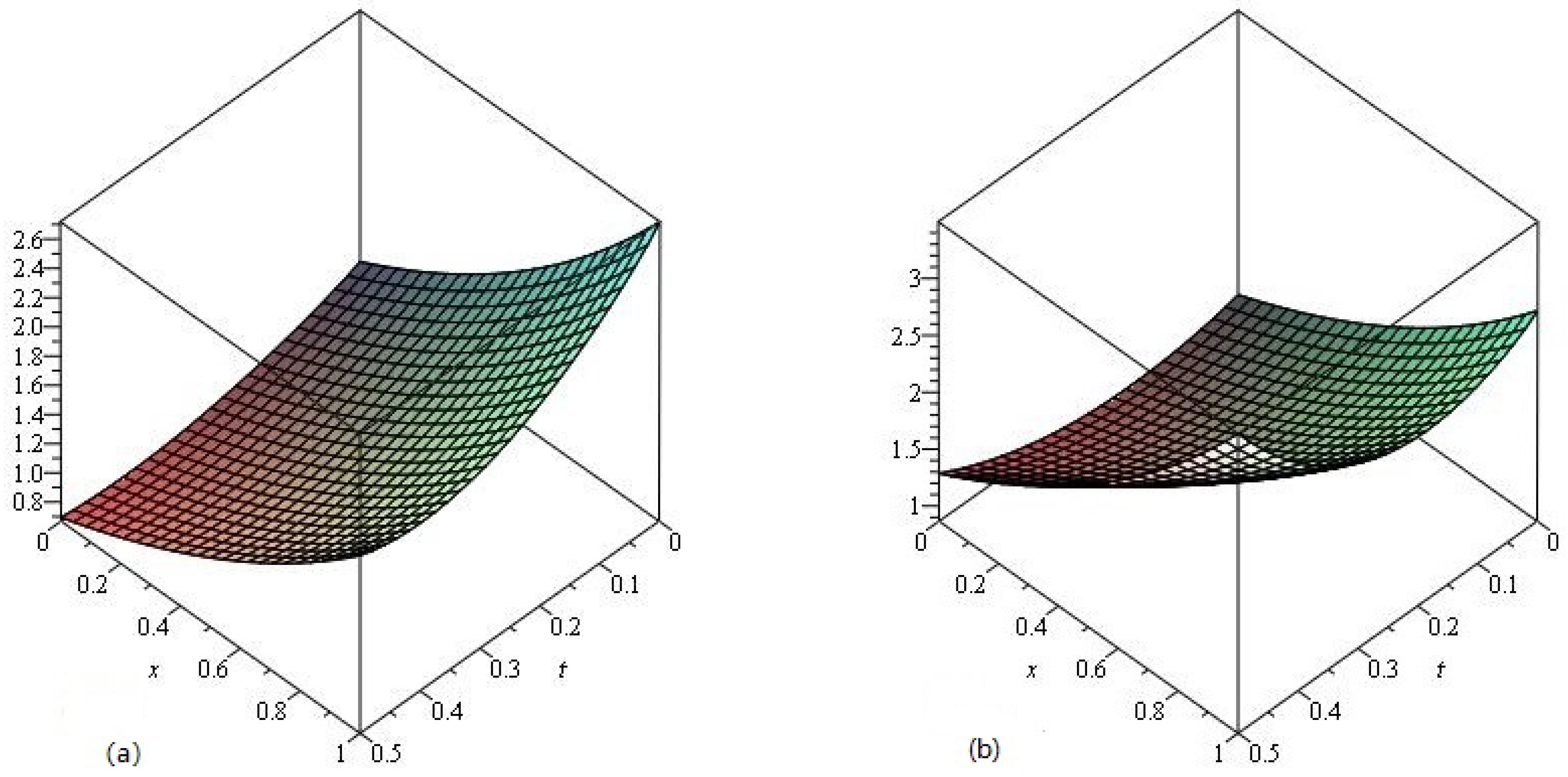
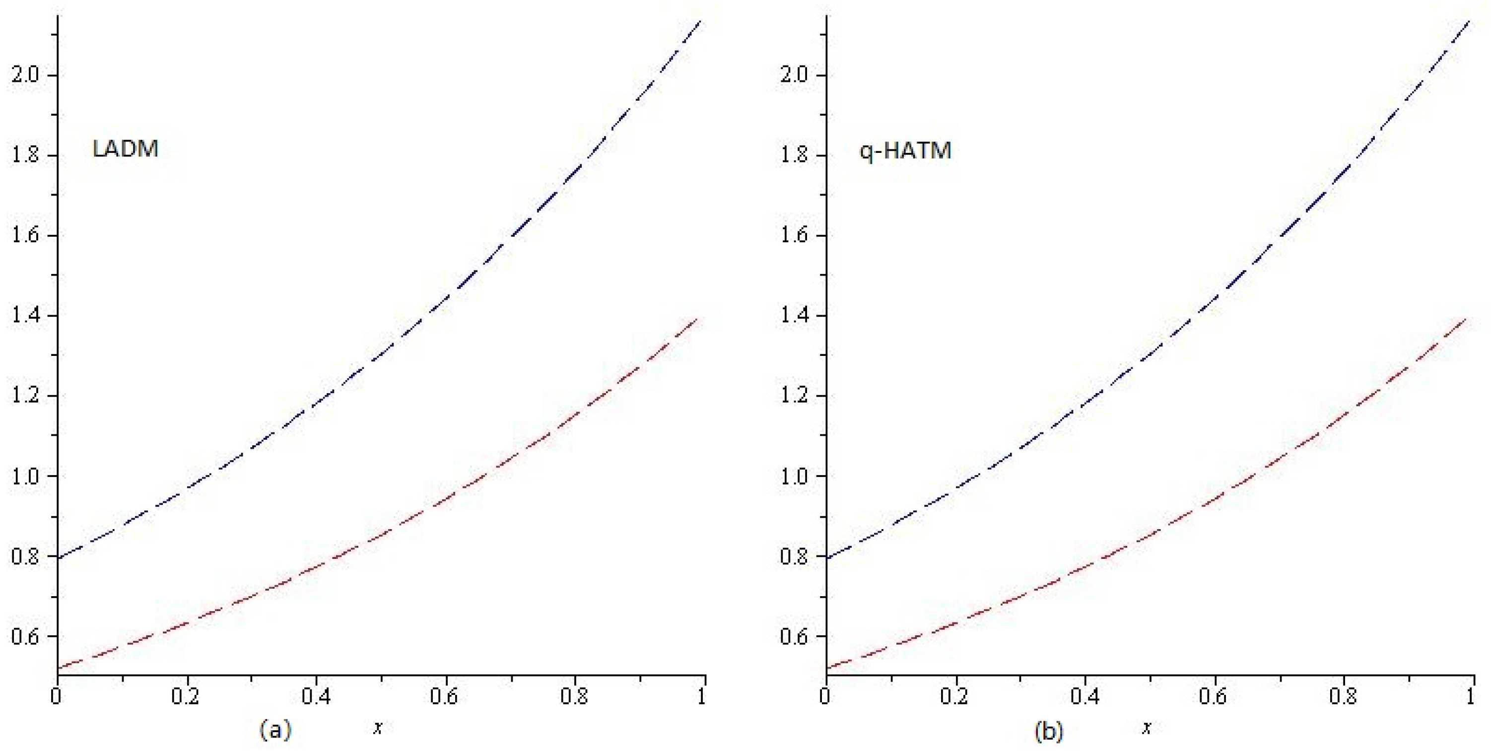
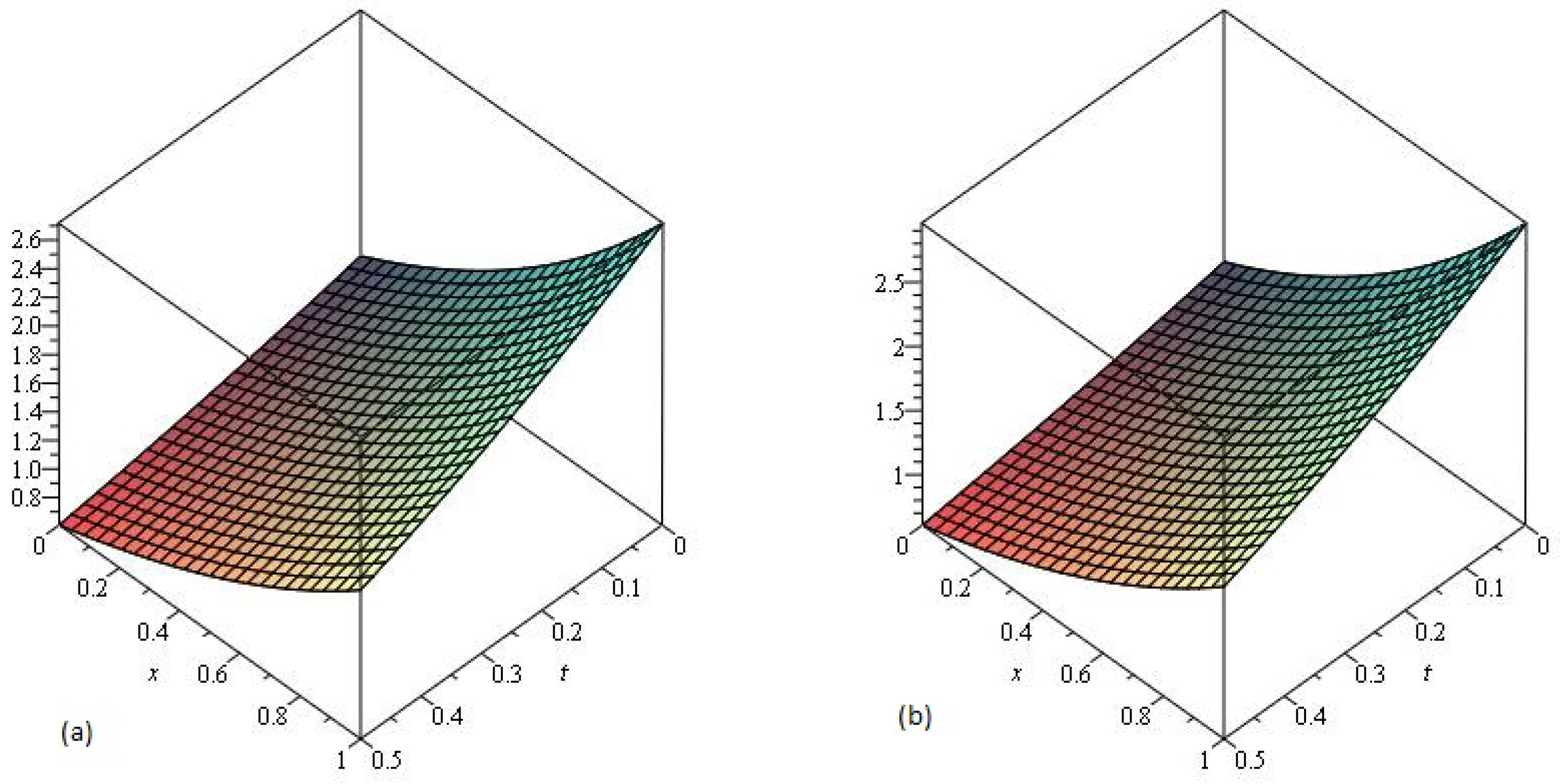
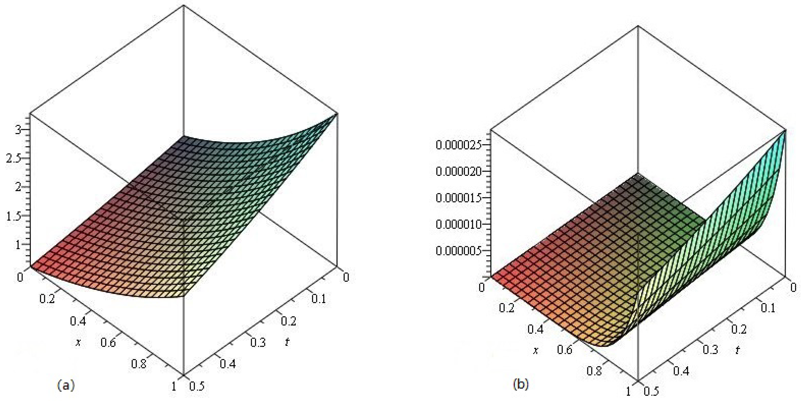
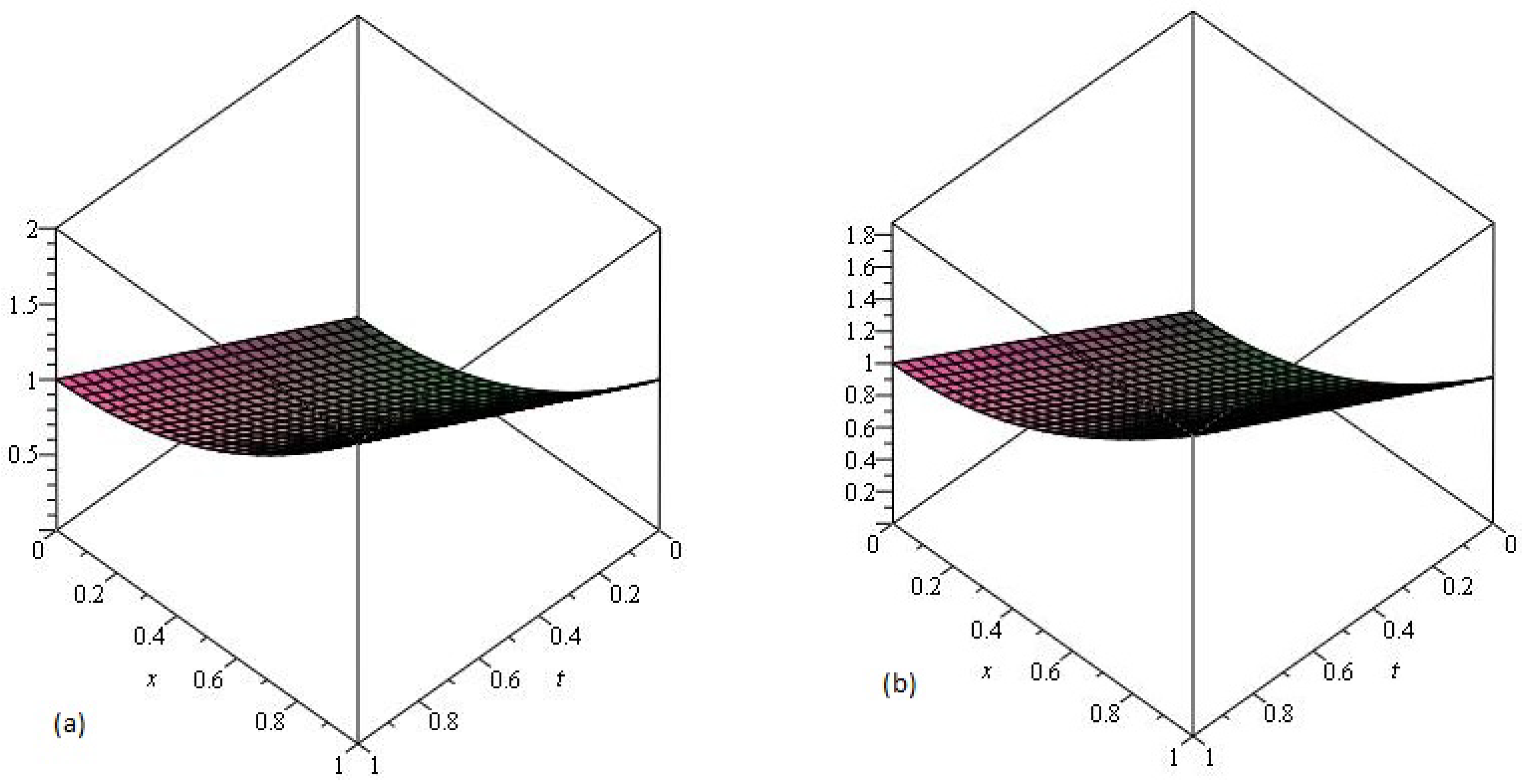
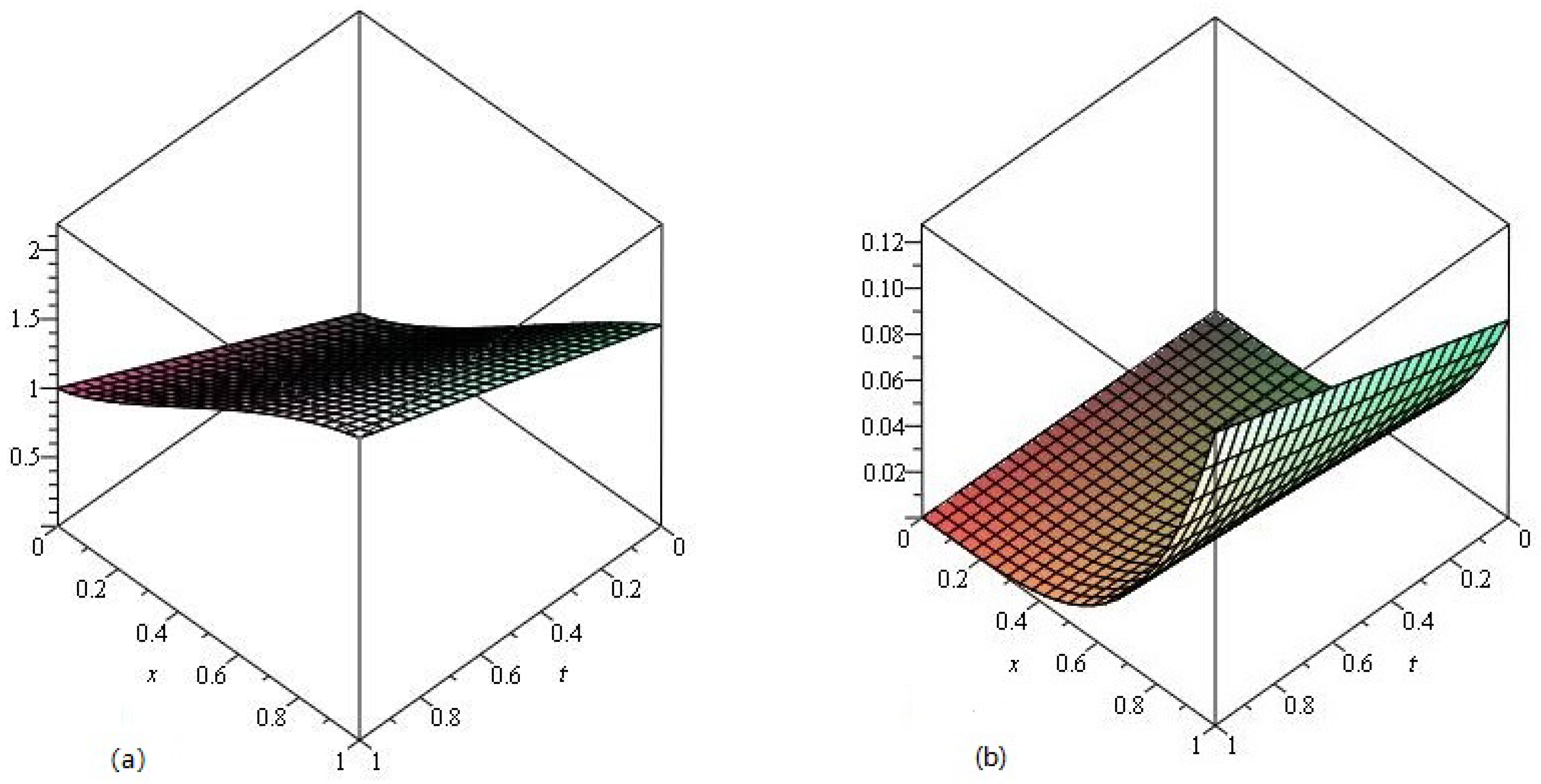
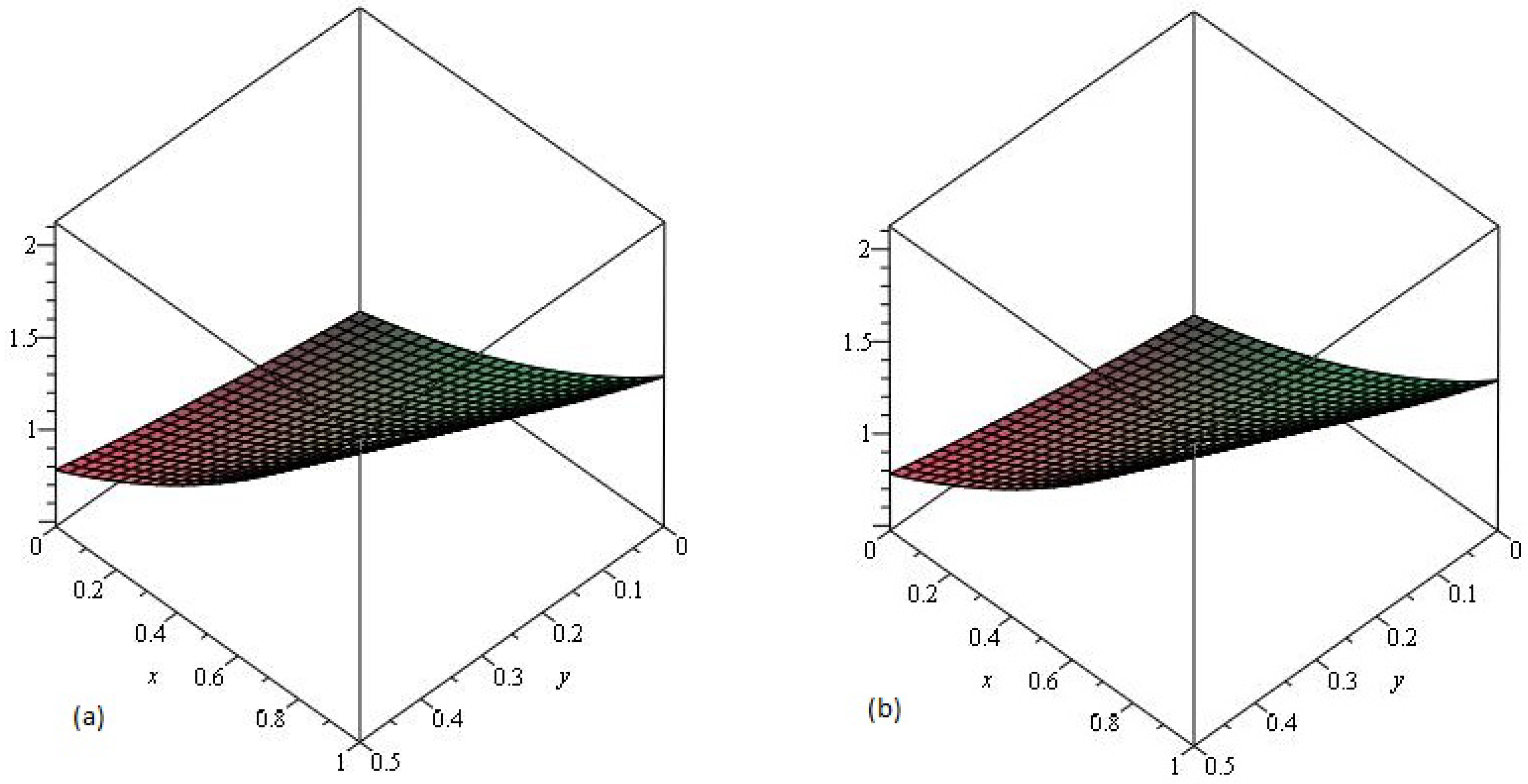
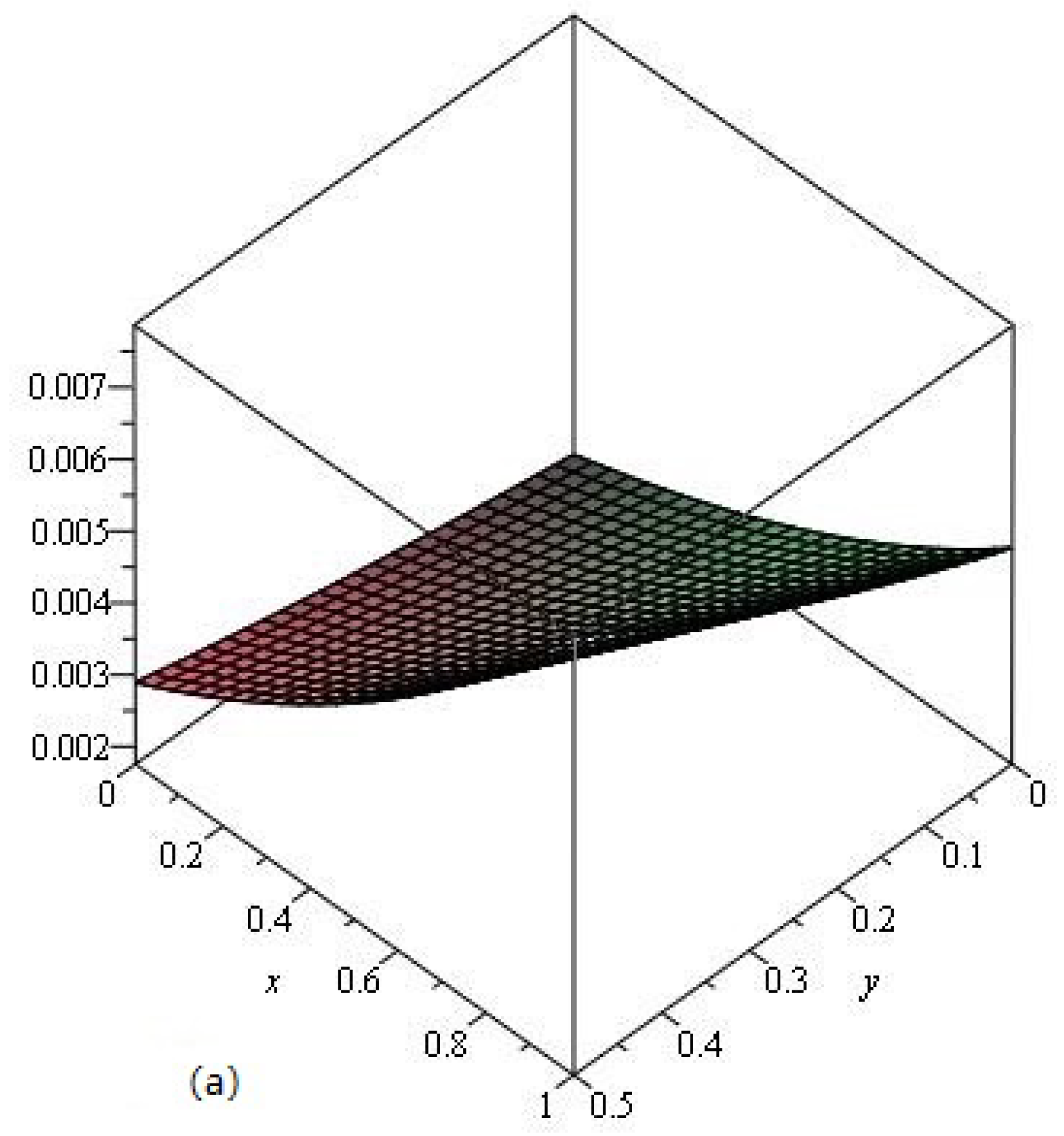
In this section, the Laplace-Adomian Decomposition Method is discussed for the solution of FPDEs.
D γ υ ( x , t ) + L υ ( x , t ) + N υ ( x , t ) = q ( x , t ) , x , t 0 , m 1 < γ < m ,
where D γ = γ t γ is the Caputo Operator γ , m N , L and N are linear and non-linear functions, and q is the source function.
The initial condition is
υ ( x , 0 ) = k ( x ) ,
Applying the Laplace transform to Equation (1), we have
L D γ υ ( x , t ) + L L υ ( x , t ) + N υ ( x , t ) = L q ( x , t ) ,
applying the fractional derivative property of the Laplace transform, we get
s γ L υ ( x , t ) s γ 1 υ ( x , 0 ) = L q ( x , t ) L L υ ( x , t ) + N υ ( x , t ) ,
L υ ( x , t ) = 1 s υ ( x , 0 ) + 1 s γ L q ( x , t ) 1 s γ L L υ ( x , t ) + N υ ( x , t ) ,
Now, υ ( x , 0 ) = k ( x )
L υ ( x , t ) = k ( x ) s + 1 s γ L q ( x , t ) 1 s γ L L υ ( x , t ) + N υ ( x , t ) .
The ADM solution υ ( x , t ) is represented by the following infinite series
υ ( x , t ) = j = 0 υ j ( x , t ) ,
and the non-linear terms (if any) in the problem are defined by the infinite series of Adomian polynomials.
N υ ( x , t ) = j = 0 A j ,
A j = 1 j ! d j d λ j N j = 0 ( λ j υ j ) λ = 0 , j = 0 , 1 , 2
substituting Equations (5) and (6) into Equation (4), we get
L j = 0 υ j ( x , t ) = k ( x ) s + 1 s γ L q ( x , t ) 1 s γ L L j = 0 υ j ( x , t ) + j = 0 A j .
Now using LADM, we have
L υ 0 ( x , t ) = k ( x ) s + 1 s γ L q ( x , t ) ,
Generally, we can write
L υ j + 1 ( x , t ) = 1 s γ L L υ j ( x , t ) + A j , j 1 .
Applying the inverse Laplace transform in Equation (9), we get
υ 0 ( x , t ) = k ( x ) + L 1 1 s γ L q ( x , t )
υ j + 1 ( x , t ) = L 1 1 s γ L L υ j ( x , t ) + A j .

4. Results

Example 1.
Consider the following time-fractional linear telegraph equation [29]:
2 γ υ t 2 γ + 2 γ υ t γ + υ = 2 υ x 2 , 0 < γ 1 , t 0 ,
with initial condition
υ ( x , 0 ) = e x , υ t ( x , 0 ) = 2 e x
Taking the Laplace transform of Equation (11),
L 2 γ υ t 2 γ = L 2 γ υ t γ + υ 2 υ x 2 ,
s 2 γ L υ ( x , t ) s 2 γ 1 υ ( x , 0 ) s 2 γ 2 υ t ( x , 0 ) = L 2 γ υ t γ + υ 2 υ x 2 .
Applying the inverse Laplace transform
υ ( x , t ) = L 1 υ ( x , 0 ) s + υ t ( x , 0 ) s 2 1 s 2 γ L 2 γ υ t γ + υ 2 υ x 2 .
Using the ADM procedure, we get:
υ 0 ( x , t ) = L 1 υ ( x , 0 ) s + υ t ( x , 0 ) s 2 = L 1 e x s 2 e x s 2
υ 0 ( x , t ) = e x ( 1 2 t )
υ j + 1 = L 1 1 s 2 γ L 2 γ υ j t γ + υ j 2 υ j x 2 , j = 0 , 1 , 2 ,
for j = 0
υ 1 ( x , t ) = L 1 1 s 2 γ L 2 γ υ 0 t γ + υ 0 2 υ 0 x 2 υ 1 ( x , t ) = L 1 4 e x s γ + 2 = 4 e x t γ + 1 Γ ( γ + 2 ) .
The subsequent terms are
υ 2 ( x , t ) = L 1 1 s 2 γ L 2 γ υ 1 t γ + υ 1 2 υ 1 x 2 = 8 e x t 2 γ + 1 Γ ( 2 γ + 2 ) , υ 3 ( x , t ) = L 1 1 s 2 γ L 2 γ υ 2 t γ + υ 2 2 υ 2 x 2 = 16 e x t 3 γ + 1 Γ ( 3 γ + 2 ) , . .
The LADM solution for Example 1 is
υ ( x , t ) = υ 0 ( x , t ) + υ 1 ( x , t ) + υ 2 ( x , t ) + υ 3 ( x , t ) + υ 4 ( x , t )
υ ( x , t ) = e x 1 2 t + 4 t γ + 1 Γ ( γ + 2 ) 8 t 2 γ + 1 Γ ( 2 γ + 2 ) + 16 t 3 γ + 1 Γ ( 3 γ + 2 ) ,
where when γ = 1 , then the LADM solution is
υ ( x , t ) = e x 1 2 t + ( 2 t ) 2 2 ! ( 2 t ) 3 3 ! + ( 2 t ) 4 4 ! .
This result is calculated to the exact solution in a closed form:
υ ( x , t ) = e x 2 t
In Figure 1, the exact solution and LADM solution of Example 1 at γ = 1 is represented by Graphs (a) and (b), respectively. From the given graphs, it can be observed that both the exact solution and LADM solution are in strong agreement with each other. In Figure 2 and Figure 3, the LADM solution of Example 1 at γ = 0.75 , 0.50 are represented by Graphs (a) and (b).
Example 2.
Consider the following time-fractional telegraph equation:
2 γ υ x 2 γ = 2 υ t 2 + υ t + υ , 1 < γ 2 , t 0 ,
with initial condition
υ ( 0 , t ) = e t , υ x ( 0 , t ) = e t
Taking the Laplace transform of (17),
L 2 γ υ x 2 γ = L 2 υ t 2 + υ t + υ ,
s 2 γ L υ ( x , t ) s 2 γ 1 υ ( 0 , t ) s 2 γ 2 υ x ( 0 , t ) = L 2 υ t 2 + υ t + υ .
Applying the inverse Laplace transform:
υ ( x , t ) = L 1 υ ( 0 , t ) s + υ x ( 0 , t ) s 2 + 1 s 2 γ L 2 υ t 2 + υ t + υ .
Using the ADM procedure, we get:
υ 0 ( x , t ) = L 1 υ ( 0 , t ) s + υ x ( 0 , t ) s 2 = L 1 e t s + e t s 2
υ 0 ( x , t ) = e t ( 1 + x )
υ j + 1 ( x , t ) = L 1 1 s 2 γ L 2 υ j t 2 + υ j t + υ j , j = 0 , 1 , 2 ,
for j = 0
υ 1 ( x , t ) = L 1 1 s 2 γ L 2 υ 0 t 2 + υ 0 t + υ 0 υ 1 ( x , t ) = L 1 e t s γ + 1 + e t s γ + 2 = e t x γ Γ ( γ + 1 ) + e t x γ + 1 Γ ( γ + 2 ) .
The subsequent terms are:
υ 2 ( x , t ) = L 1 1 s 2 γ L 2 υ 1 t 2 + υ 1 t + υ 1 = e t x 2 γ Γ ( 2 γ + 1 ) + e t x 2 γ + 1 Γ ( 2 γ + 2 ) , υ 3 ( x , t ) = L 1 1 s 2 γ L 2 υ 2 t 2 + υ 2 t + υ 2 = e t x 3 γ Γ ( 3 γ + 1 ) + e t x 3 γ + 1 Γ ( 3 γ + 2 ) , . .
The LADM solution for Example 4.2 is:
υ ( x , t ) = υ 0 ( x , t ) + υ 1 ( x , t ) + υ 2 ( x , t ) + υ 3 ( x , t ) + υ 4 ( x , t )
υ ( x , t ) = e t [ 1 + x + x γ Γ ( γ + 1 ) + x γ + 1 Γ ( γ + 2 ) + x 2 γ Γ ( 2 γ + 1 ) + x 2 γ + 1 Γ ( 2 γ + 2 ) + x 3 γ Γ ( 3 γ + 1 ) + x 3 γ + 1 Γ ( 3 γ + 2 ) ] ,
when γ = 2 , the LADM solution is
υ ( x , t ) = e t 1 + x + x 2 2 ! + x 3 3 ! + x 4 4 ! + x 5 5 ! .
This result was calculated to the exact solution in a closed form:
υ ( x , t ) = e x t
In Figure 4, the LADM solution of Example 2 at γ = 1 , γ = 0.75 are represented by Graphs (a) and (b), respectively. From the given graphs, it can be observed that both the exact and LADM solutions are in strong agreement with each other. In Figure 5, the LADM solution of Example 2 at γ = 0.75 is represented by graph (a) and error graph (b) at γ = 1 , respectively.
Example 3.
Consider the following non-homogeneous space-time fractional telegraph equation:
γ υ x γ = 2 υ t 2 + υ t + υ x 2 t + 1 , 0 < γ 1 , t 0 ,
with initial condition
υ ( 0 , t ) = t , υ x ( 0 , t ) = 0 .
Taking the Laplace transform of (23),
L γ υ x γ = L 2 υ t 2 + υ t + υ x 2 t + 1 ,
s γ L υ ( x , t ) s γ 1 υ ( 0 , t ) s γ 2 υ x ( 0 , t ) = L 2 υ t 2 + υ t + υ x 2 t + 1 .
Applying the inverse Laplace transform
υ ( x , t ) = L 1 υ ( 0 , t ) s + υ x ( 0 , t ) s 2 2 s γ + 3 t s γ + 1 + 1 s γ + 1 + 1 s γ L 2 υ t 2 + υ t + υ .
Using the ADM procedure, we get
υ 0 ( x , t ) = L 1 υ ( 0 , t ) s + υ x ( 0 , t ) s 2 2 s γ + 3 t s γ + 1 + 1 s γ + 1 ,
υ 0 ( x , t ) = L 1 t s 2 s γ + 3 t s γ + 1 + 1 s γ + 1
υ 0 ( x , t ) = t 2 x γ + 2 Γ ( γ + 3 ) t x γ Γ ( γ + 1 ) + x γ Γ ( γ + 1 )
υ j + 1 ( x , t ) = L 1 1 s γ L 2 υ j t 2 + υ j t + υ j , j = 0 , 1 , 2 ,
for j = 0
υ 1 ( x , t ) = L 1 1 s 2 γ L 2 υ 0 t 2 + υ 0 t + υ 0 υ 1 ( x , t ) = x γ Γ ( γ + 1 ) + t x γ Γ ( γ + 1 ) 2 x 2 γ + 2 Γ ( 2 γ + 3 ) t x 2 γ Γ ( 2 γ + 1 ) .
The LADM solution for Example 3 is
υ ( x , t ) = [ t 2 x γ + 2 Γ ( γ + 3 ) + 2 x γ Γ ( γ + 1 ) 2 x 2 γ + 2 Γ ( 2 γ + 3 ) t x 2 γ Γ ( 2 γ + 1 ) ] ,
when γ = 1 , then the LADM solution is
υ ( x , t ) = t + 2 x 2 x 2 2 ! 2 x 3 3 ! 2 x 4 4 ! .
This result is calculated to the exact solution in a closed form;
υ ( x , t ) = t + x 2
In Figure 6, the LADM solution of Example 3 at γ = 1 , γ = 0.75 are represented by Graphs (a) and (b), respectively. From the given graphs it can be observed that both exact and LADM solutions are in strong agreement with each other. In Figure 7 the LADM solution of Example 3 at γ = 0.75 are represented by graph (a) and Error graph (b) at γ = 1 , respectively.
Example 4.
Consider the linear time-fractional linear telegraph equation:
2 γ υ t 2 γ + 3 γ υ t γ + 2 υ = 2 υ x 2 + 2 υ y 2 , 0 < γ 1 , t 0 ,
with initial condition
υ ( x , y , 0 ) = e x + y , υ t ( x , y , 0 ) = 3 e x + y
Taking the Laplace transform of Equation (28),
L 2 γ υ t 2 γ = L 3 γ υ t γ + 2 υ 2 υ x 2 2 υ y 2 ,
s 2 γ L υ ( x , y , t ) s 2 γ 1 υ ( x , y , 0 ) s 2 γ 2 υ t ( x , y , 0 ) = L 3 γ υ t γ + 2 υ 2 υ x 2 2 υ y 2 .
Applying the inverse Laplace transform
υ ( x , y , t ) = L 1 υ ( x , y , 0 ) s + υ t ( x , y , 0 ) s 2 1 s 2 γ L 3 γ υ t γ + 2 υ 2 υ x 2 2 υ y 2 .
Using the ADM procedure, we get
υ 0 ( x , y , t ) = L 1 υ ( x , y , 0 ) s + υ t ( x , y , 0 ) s 2 = L 1 e x + y s 3 e x + y s 2
υ 0 ( x , y , t ) = e x + y ( 1 3 t )
υ j + 1 ( x , y , t ) = L 1 1 s 2 γ L 3 γ υ j t γ + 2 υ j 2 υ j x 2 2 υ j y 2 , j = 0 , 1 , 2 ,
for j = 0
υ 1 ( x , y , t ) = L 1 1 s 2 γ L 3 γ υ 0 t γ + 2 υ 0 2 υ 0 x 2 2 υ 0 y 2 υ 1 ( x , y , t ) = L 1 9 e x + y s γ + 2 = 9 e x + y t γ + 1 Γ ( γ + 2 ) .
The subsequent terms are
υ 2 ( x , t ) = L 1 1 s 2 γ L 3 γ υ 1 t γ + 2 υ 1 2 υ 1 x 2 2 υ 1 y 2 = 27 e x + y t 2 γ + 1 Γ ( 2 γ + 2 ) , υ 3 ( x , t ) = L 1 1 s 2 γ L 3 γ υ 2 t γ + 2 υ 2 2 υ 2 x 2 2 υ 2 y 2 = 81 e x + y t 3 γ + 1 Γ ( 3 γ + 2 ) , . .
The LADM solution for Example 4 is
υ ( x , y , t ) = υ 0 ( x , t ) + υ 1 ( x , t ) + υ 2 ( x , t ) + υ 3 ( x , t ) + υ 4 ( x , t )
υ ( x , t ) = e x + y 1 3 t + 9 t γ + 1 Γ ( γ + 2 ) 27 t 2 γ + 1 Γ ( 2 γ + 2 ) + 81 t 3 γ + 1 Γ ( 3 γ + 2 ) ,
when γ = 1 , then LADM solution is
υ ( x , y , t ) = e x + y 1 3 t + ( 3 t ) 2 2 ! ( 3 t ) 3 3 ! + ( 3 t ) 4 4 ! .
This result is calculated to the exact solution in a closed form;
υ ( x , y , t ) = e x + y 3 t
In Figure 8, the exact and LADM solutions of Example 4 at γ = 1 are represented by Graphs (a) and (b), respectively. From the given graphs it can be observed that both exact and LADM solutions are in strong agreement with each other. In Figure 9 and Figure 10, the LADM solution of Example 4 at γ = 0.75 , 0.50 is represented by graph (a), graph (b), and Error graph (a) at γ = 1 , respectively.
Example 5.
Consider the linear time-fractional linear telegraph equation:
2 γ υ t 2 γ + 2 γ υ t γ + 3 υ = 2 υ x 2 + 2 υ y 2 + 2 υ z 2 , 0 < γ 1 , t 0 ,
with initial condition
υ ( x , y , z , 0 ) = sinh ( x ) sinh ( y ) sinh ( z ) , υ t ( x , y , z , 0 ) = sinh ( x ) sinh ( y ) sinh ( z )
Taking the Laplace transform of Equation (34),
L 2 γ υ t 2 γ = L 2 γ υ t γ + 3 υ 2 υ x 2 2 υ y 2 2 υ z 2 ,
s 2 γ L υ ( x , y , z , t ) s 2 γ 1 υ ( x , y , z , 0 ) s 2 γ 2 υ t ( x , y , z , 0 ) = L 2 γ υ t γ + 3 υ 2 υ x 2 2 υ y 2 2 υ z 2 .
Applying the inverse Laplace transform
υ ( x , y , z , t ) = L 1 υ ( x , y , z , 0 ) s + υ t ( x , y , z , 0 ) s 2 L 1 1 s 2 γ L 2 γ υ t γ + 3 υ 2 υ x 2 2 υ y 2 2 υ z 2 .
Using the ADM procedure, we get
υ 0 ( x , y , z , t ) = L 1 υ ( x , y , z , 0 ) s + υ t ( x , y , z , 0 ) s 2 = L 1 sinh ( x ) sinh ( y ) sinh ( z ) s sinh ( x ) sinh ( y ) sinh ( z ) s 2
υ 0 ( x , y , z , t ) = sinh ( x ) sinh ( y ) sinh ( z ) ( 1 t )
υ j + 1 ( x , y , z , t ) = L 1 1 s 2 γ L 2 γ υ j t γ + 3 υ j 2 υ j x 2 2 υ j y 2 2 υ j z 2 , j = 0 , 1 , 2 ,
for j = 0
υ 1 ( x , y , z , t ) = L 1 1 s 2 γ L 2 γ υ 0 t γ + 3 υ 0 2 υ 0 x 2 2 υ 0 y 2 2 υ 0 z 2 υ 1 ( x , y , z , t ) = L 1 2 sinh ( x ) sinh ( y ) sinh ( z ) s γ + 2 υ 1 ( x , y , z , t ) = 2 sinh ( x ) sinh ( y ) sinh ( z ) t γ + 1 Γ ( γ + 2 )
The subsequent terms are
υ 2 ( x , y , z , t ) = L 1 1 s 2 γ L 2 γ υ 1 t γ + 3 υ 1 2 υ 1 x 2 2 υ 1 y 2 2 υ 1 z 2 υ 2 ( x , y , z , t ) = 4 sinh ( x ) sinh ( y ) sinh ( z ) t 2 γ + 1 Γ ( 2 γ + 2 ) , υ 3 ( x , y , z , t ) = L 1 1 s 2 γ L 2 γ υ 2 t γ + 3 υ 2 2 υ 2 x 2 2 υ 2 y 2 2 υ 2 z 2 υ 3 ( x , y , z , t ) = 8 sinh ( x ) sinh ( y ) sinh ( z ) t 3 γ + 1 Γ ( 3 γ + 2 ) , . .
The LADM solution for Example 5 is
υ ( x , y , z , t ) = υ 0 ( x , y , z , t ) + υ 1 ( x , y , z , t ) + υ 2 ( x , y , z , t ) + υ 3 ( x , y , z , t )
υ ( x , y , z , t ) = sinh ( x ) sinh ( y ) sinh ( z ) 1 + t 2 t γ + 1 Γ ( γ + 2 ) + 4 t 2 γ + 1 Γ ( 2 γ + 2 ) 8 t 3 γ + 1 Γ ( 3 γ + 2 ) ,
This result was calculated to the exact solution in a closed form:
υ ( x , y , z , t ) = e 2 t sinh ( x ) sinh ( y ) sinh ( z )
In Figure 11, the exact and LADM solution of Example 5 at γ = 1 are represented by Graphs (a) and (b), respectively. From the given graphs it can be observed that both exact and LADM solutions are in strong agreement with each other. In Figure 12 the LADM solution of Example 5 at γ = 0.75 are represented by graph (a) and Error graph (b) at γ = 1 , respectively.

5. Conclusions

In this paper, the analytical solutions of telegraph equations and fractional partial differential equations were determined using LADM. The fractional derivatives were described by using the Caputo operator. For the LADM, solutions were obtained at fractional and integer orders for all problems. The results revealed the highest agreement with the exact solutions for the problems. For some numerical examples, the LADM solutions showed the validity of the proposed method. It is also showed that the fractional order solutions were convergent to the exact solution for the problems, as the fractional order approaches the integer order. The implementation of LADM to illustrative examples have also confirmed that the fractional-order mathematical model can be the best representation of any experimental data as compared to the integer-order model. Moreover, by taking different fractional orders, we were able to find a way to set suitable mathematical models for any experimental data, and thus find reasonable consequences. Hence, it is concluded that LADM is the best tool for the solution of FPDEs, as compared to ADM and DTM in the literature. LADM was found to provide the highest rate of convergence to the exact solution for the problems. In future, LADM can be used to find the analytical solution of other non-linear FPDEs, which are frequently used in science and engineering. LADM solutions for fractional-order problems will prove to give the best understanding of real-world problems presented by FPDEs.

Author Contributions

Conceptualization, R.S. and H.K.; Methodology, M.A.; Software, R.S.; Validation, D.B. and M.A.; Formal Analysis, R.S.; Investigation, R.S. and P.K.; Resources, H.K. and P.K.; Data Curation, R.S.; Writing—Original Draft Preparation, R.S.; Writing—Review and Editing, H.K., D.B. and P.K.; Visualization, M.A.; Supervision, M.A., P.K.; Project Administration, P.K.; Funding Acquisition, P.K.

Funding

The project was supported by the Center of Excellence in Theoretical and Computational Science (TaCS-CoE), Faculty of Science, King Mongkut’s University of Technology Thonburi (KMUTT).

Acknowledgments

This project was supported by the Theoretical and Computational Science (TaCS) Center under Computational and Applied Science for Smart Innovation Research Cluster (CLASSIC), Faculty of Science, KMUTT.

Conflicts of Interest

The authors declare no conflict of interest.

References

  1. Hilfer, R. Applications of Fractional Calculus in Physics; World Sci. Publishing: River Edge, NJ, USA, 2000. [Google Scholar]
  2. Podlubny, I. Fractional Differential Equations: An Introduction to Fractional Derivatives, Fractional Differential Equations, to Methods of Their Solution and Some of Their Applications; Elsevier: Amsterdam, The Netherlands, 1998; Volume 198. [Google Scholar]
  3. Miller, K.S.; Ross, B. An Introduction to the Fractional Calculus and Fractional Differential Equations; Wiley: Hoboken, NJ, USA, 1993; p. 384. [Google Scholar]
  4. Bildik, N.; Konuralp, A. The use of variational iteration method, differential transform method and Adomian decomposition method for solving different types of nonlinear partial differential equations. Int. J. Nonlinear Sci. Numer. Simul. 2006, 7, 65–70. [Google Scholar] [CrossRef]
  5. Gómez-Aguilar, J.F.; Yépez-Martínez, H.; Torres-Jiménez, J.; Córdova-Fraga, T.; Escobar-Jiménez, R.F.; Olivares-Peregrino, V.H. Homotopy perturbation transform method for nonlinear differential equations involving to fractional operator with exponential kernel. Adv. Differ. Equations 2017, 2017, 68. [Google Scholar] [CrossRef]
  6. Atangana, A.; Gómez-Aguilar, J.F. Numerical approximation of Riemann-Liouville definition of fractional derivative: From Riemann-Liouville to Atangana-Baleanu. Numer. Methods Partial. Differ. Equations 2018, 34, 1502–1523. [Google Scholar] [CrossRef]
  7. Kilbas, A.A.A.; Srivastava, H.M.; Trujillo, J.J. Theory and Applications of Fractional Differential Equations; Elsevier Science Limited: Amsterdam, The Netherlands, 2006; Volume 204. [Google Scholar]
  8. Jiang, J.; Feng, Y.; Li, S. Exact Solutions to the Fractional Differential Equations with Mixed Partial Derivatives. Axioms 2018, 7, 10. [Google Scholar] [CrossRef]
  9. Silva, F.; Moreira, D.; Moret, M. Conformable Laplace Transform of Fractional Differential Equations. Axioms 2018, 7, 55. [Google Scholar] [CrossRef]
  10. Machado, J.T. Entropy analysis of integer and fractional dynamical systems. Nonlinear Dyn. 2010, 62, 371–378. [Google Scholar]
  11. Ball, J.M.; Chen, G.Q.G. Entropy and Convexity for Nonlinear Partial Differential Equations. Philos. Trans. A Math. Phys. Eng. Sci. 2013, 371, 2005. [Google Scholar] [CrossRef] [PubMed]
  12. Lopes, A.M.; Tenreiro Machado, J.A. Entropy Analysis of Soccer Dynamics. Entropy 2019, 21, 187. [Google Scholar] [CrossRef]
  13. Yavuz, M.; Özdemir, N. European vanilla option pricing model of fractional order without singular kernel. Fractal Fract. 2018, 2, 3. [Google Scholar] [CrossRef]
  14. Thabet, H.; Kendre, S.; Chalishajar, D. New analytical technique for solving a system of nonlinear fractional partial differential equations. Mathematics 2017, 5, 47. [Google Scholar] [CrossRef]
  15. Daftardar-Gejji, V.; Jafari, H. An iterative method for solving nonlinear functional equations. J. Math. Anal. Appl. 2006, 316, 753–763. [Google Scholar] [CrossRef]
  16. Jafari, H. Iterative Methods for Solving System of Fractional Differential Equations. Ph.D. Thesis, Pune University, Pune City, India, 2006. [Google Scholar]
  17. Ali, A.; Shah, K.; Khan, R.A. Numerical treatment for traveling wave solutions of fractional Whitham-Broer-Kaup equations. Alex. Eng. J. 2018, 57, 1991–1998. [Google Scholar] [CrossRef]
  18. Ahmed, H.F.; Bahgat, M.S.; Zaki, M. Numerical approaches to system of fractional partial differential equations. J. Egypt. Math. Soc. 2017, 25, 141–150. [Google Scholar] [CrossRef]
  19. Irfan, N.; Kumar, S.; Kapoor, S. Bernstein Operational Matrix Approach for Integro-Differential Equation Arising in Control theory. Nonlinear Eng. Nonlinear Eng. 2014, 3, 117–123. [Google Scholar]
  20. Yousef, H.M.; Ismail, A.M. Application of the Laplace Adomian decomposition method for solution system of delay differential equations with initial value problem. Aip Conf. Proc. 2018, 1974, 020038. [Google Scholar]
  21. Jafari, H.; Khalique, C.M.; Nazari, M. Application of the Laplace decomposition method for solving linear and nonlinear fractional diffusion–wave equations. Appl. Math. Lett. 2011, 24, 1799–1805. [Google Scholar] [CrossRef]
  22. Mohamed, M.Z.; Elzaki, T.M. Comparison between the Laplace Decomposition Method and Adomian Decomposition in Time-Space Fractional Nonlinear Fractional Differential Equations. Appl. Math. 2018, 9, 448–458. [Google Scholar] [CrossRef]
  23. Shah, R.; Khan, H.; Arif, M.; Kumam, P. Application of Laplace–Adomian Decomposition Method for the Analytical Solution of Third-Order Dispersive Fractional Partial Differential Equations. Entropy 2019, 21, 335. [Google Scholar] [CrossRef]
  24. Okubo, A. Application of the Telegraph Equation to Oceanic Diffusion: Another Mathematic Model; Chesapeake bay institute, The Johns Hopking Unversity: Baltimore, MD, USA, 1971; p. 42. [Google Scholar]
  25. Javidi, M.; Nyamoradi, N. Numerical solution of telegraph equation by using LT inversion technique. Int. J. Adv. Math. Sci. 2013, 1, 64–77. [Google Scholar] [CrossRef]
  26. Veeresha, P.; Prakasha, D.G. Numerical solution for fractional model of telegraph equation by using q-HATM. arXiv 2018, arXiv:1805.03968. [Google Scholar]
  27. Al-badrani, H.; Saleh, S.; Bakodah, H.O.; Al-Mazmumy, M. Numerical Solution for Nonlinear Telegraph Equation by Modified Adomian Decomposition Method. Nonlinear Anal. Differ. Equations 2016, 4, 243–257. [Google Scholar] [CrossRef]
  28. Srivastava, V.K.; Awasthi, M.K.; Chaurasia, R.K.; Tamsir, M. The telegraph equation and its solution by reduced differential transform method. Model. Simul. Eng. 2013, 2013. [Google Scholar] [CrossRef]
  29. Srivastava, V.K.; Awasthi, M.K.; Tamsir, M. RDTM solution of Caputo time fractional-order hyperbolic telegraph equation. Aip Adv. 2013, 3, 032142. [Google Scholar] [CrossRef]
  30. Inc, M.; Akgül, A.; Kiliçman, A. Explicit solution of telegraph equation based on reproducing kernel method. J. Funct. Spaces Appl. 2012, 2012. [Google Scholar] [CrossRef]
  31. Biazar, J.; Ebrahimi, H.; Ayati, Z. An approximation to the solution of telegraph equation by variational iteration method. Numer. Methods Partial. Differ. Equations 2009, 25, 797–801. [Google Scholar] [CrossRef]
  32. Erfanian, M.; Gachpazan, M. A new method for solving of telegraph equation with Haar wavelet. Int. J. Math. Comput. Sci. 2016, 3, 6–10. [Google Scholar]
  33. Latifizadeh, H. The sinc-collocation method for solving the telegraph equation. J. Comput. Inform. 2013, 1, 13–17. [Google Scholar]
  34. Jiwari, R.; Pandit, S.; Mittal, R.C. A differential quadrature algorithm for the numerical solution of the second-order one dimensional hyperbolic telegraph equation. Int. J. Nonlinear Sci. 2012, 13, 259–266. [Google Scholar]
  35. Wang, Y.; Mei, L. Generalized finite difference/spectral Galerkin approximations for the time-fractional telegraph equation. Adv. Differ. Equations 2017, 2017, 281. [Google Scholar] [CrossRef]
  36. Kumar, D.; Singh, J.; Kumar, S. Analytic and approximate solutions of space-time fractional telegraph equations via Laplace transform. Walailak J. Sci. Technol. 2013, 11, 711–728. [Google Scholar]
Figure 1. The (a) Exact and (b) LADM solutions of υ ( x , t ) of Example 1 a t γ = 1 .
Mathematics 07 00426 g001
Figure 2. The LADM solution of υ ( x , t ) of Example 1 a t (a) γ = 0.75 and (b) a t γ = 0.50 .
Mathematics 07 00426 g002
Figure 3. The comparison plots a t γ = 0.75 and 0.50 .
Mathematics 07 00426 g003
Figure 4. The (a) LADM solutions of υ ( x , t ) of Example 2 a t γ = 1 and (b) γ = 0.75 .
Mathematics 07 00426 g004
Figure 5. The LADM solution of υ ( x , t ) of Example 2 a t (a) γ = 0.50 and (b) Error plot a t γ = 1 .
Mathematics 07 00426 g005
Figure 6. The (a) Exact and (b) LADM solutions of υ ( x , t ) of Example 4.3, a t γ = 1 .
Mathematics 07 00426 g006
Figure 7. The LADM solution of υ ( x , t ) of Example 3, a t (a) γ = 0.50 and (b) Error plot a t γ = 1 .
Mathematics 07 00426 g007
Figure 8. The (a) Exact and (b) LADM solutions of υ ( x , y , t ) of Example 4 a t γ = 1 .
Mathematics 07 00426 g008
Figure 9. The LADM solution of υ ( x , y , t ) of Example 4.4 a t (a) γ = 0.75 and (b) a t γ = 0.50 .
Mathematics 07 00426 g009
Figure 10. The (a) Error plot of υ ( x , y , t ) of Example 4 a t γ = 1 .
Mathematics 07 00426 g010
Figure 11. The (a) Exact and (b) LADM solutions of υ ( x , y , z , t ) of Example 4.5, a t γ = 1 .
Mathematics 07 00426 g011
Figure 12. The LADM solution of υ ( x , y , z , t ) of Example 4.5 at (a) γ = 0.50 and (b) Error plot at γ = 1 .
Mathematics 07 00426 g012

