Abstract
This paper is concerned with the joint state and parameter estimation methods for a bilinear system in the state space form, which is disturbed by additive noise. In order to overcome the difficulty that the model contains the product term of the system input and states, we make use of the hierarchical identification principle to present new methods for estimating the system parameters and states interactively. The unknown states are first estimated via a bilinear state estimator on the basis of the Kalman filtering algorithm. Then, a state estimator-based recursive generalized least squares (RGLS) algorithm is formulated according to the least squares principle. To improve the parameter estimation accuracy, we introduce the data filtering technique to derive a data filtering-based two-stage RGLS algorithm. The simulation example indicates the efficiency of the proposed algorithms.
1. Introduction
Nonlinear systems widely exist in practical industrial processes. Employing mathematical models of these processes becomes increasingly significant in system analysis [1,2,3], system control [4,5,6] and signal processing [7,8,9,10], so it is necessary to find efficient methods for system modeling [11,12,13]. Mathematical modeling methods are summarized into three categories, including mechanism modeling, experimental modeling, and their combination [14,15,16,17]. System identification is the field of getting appropriate models of dynamic systems directly from experimental data [18,19,20,21] and can be applied to many areas [22,23,24,25,26]. As a special class of nonlinear systems, bilinear systems are capable of approximately describing some complex dynamic processes such as a nuclear reactor, the heat transform process, and biology [27,28,29]. As a result, there are many active researches towards the parameter estimation problem of bilinear systems [30,31].
In the literature of bilinear system identification, Verdult and Verhaegen applied the subspace identification techniques for multi-input multi-output bilinear systems by using the separable least squares principle [32]. Larkowski et al. handled the parameter estimation problem of the diagonal bilinear errors-in-variables system and employed the bias-compensated least squares method to estimate the parameters [33]. Hizir et al. transformed a bilinear system into its equivalent linear model and used the observer Kalman filter identification algorithm to identify the bilinear system [34]. Vicario et al. extended the interaction matrices to bilinear systems to present the relationship between the system states and the measurement data and developed the intersection subspace algorithm for the bilinear system identification [35].
The recursive least squares (RLS) method is regarded as the common parameter estimation approach among many different parameter estimation techniques [36,37,38]. Gan et al. proposed an efficient variable projection method to solve nonlinear least squares problems based on the matrix decomposition [39]. Compared with the transfer function representation [40,41], the state space model can reflect the motion of the inner mechanism and cover state estimation [42,43,44]. Many estimation methods such as sequential Monte Carlo methods [45] and subspace identification methods [46] have been extensively applied in many areas. Stroud et al. proposed a Bayesian method for the joint state and parameter estimation of state space models with additive Gaussian noise using the ensemble Kalman filter [47]. Urteaga et al. presented a sequential Monte Carlo method for filtering and prediction of time-varying signals by fusing the information from candidate models instead of using model selection [48]. Martino et al. presented the parallel particle filters based on the Bayesian model averaging principle for sequential tracking and online model selection [49]. Schön et al. derived an expectation maximization algorithm under the maximum likelihood framework and gave the parameter estimates of nonlinear state space models [50]. Li and Liu derived the input-output representation of the bilinear system through eliminating the state variables and proposed the filtering-based least squares iterative algorithm [51]. However, the state variables in the system were eliminated, so the state estimation of the bilinear system was not studied.
The bilinear system involves the products of control inputs and state variables in the state equation. Thus, linear system identification methods cannot be utilized to compute the parameter estimates due to the unmeasurable states. Different from the work in [51], this paper focuses on the joint parameter and state estimation problem for a bilinear state space system with colored noise. The bilinear model can be regarded as a time-varying state space model [52]. Thus, this paper presents a bilinear state estimator based on the Kalman filtering algorithm for computing the unknown states. Then, the state estimator-based recursive generalized least squares (RGLS) identification algorithm is developed for estimating the system parameters according to the least squares principle. For the purpose of improving the parameter estimation accuracy, the data filtering technique is introduced by transforming the bilinear model into several filtered submodels with smaller dimensions. The main contributions of this paper are listed as follows.
- We present a bilinear state estimator on the basis of the Kalman filtering algorithm.
- We derive a state estimator-based RGLS algorithm for joint state and parameter estimation of bilinear state space models on the basis of the hierarchical identification principle.
- We derive a filtering-based two-stage RGLS (F-TS-RGLS) algorithm using the state estimates for improving the parameter estimation accuracy by introducing the data filtering technique.
The remainder of this paper is organized as follows. Section 2 describes the bilinear system and gives its identification model. Section 3 derives a state estimator-based RGLS identification algorithm. Section 4 presents a state estimator-based F-TS-RGLS algorithm by using the data filtering technique. Section 5 provides an illustrative example to demonstrate the effectiveness of the proposed algorithms. Finally, some conclusions are given in Section 6.
2. System Description
Some symbols are introduced for convenience. “” or “” stands for “A is defined as X”; denotes the estimate of at time t; the symbol () represents an identity matrix of an appropriate size (); z denotes a unit forward shift operator like and ; the superscript T symbolizes the matrix/vector transpose.
Recently, a state observer-based multi-innovation stochastic gradient algorithm and a state observer-based recursive least squares identification algorithm were presented for a bilinear system with white noise [53]:
Zhang et al. derived a state filtering-based hierarchical identification algorithm and a state filtering-based forgetting factor recursive least squares algorithm for a bilinear system with white noise [54]:
On the basis of the data filtering technique, a bilinear state observer-based multi-innovation extended stochastic gradient algorithm and a data filtering-based multi-innovation extended stochastic gradient algorithm were developed for a bilinear system with moving average noise [55]:
where .
Different from the work in [53,54,55], this paper considers a single-input single-output bilinear system with autoregressive noise:
where is the state vector, and are the system input and output data, is the measurement noise, and , , , and are the system parameters:
Without loss of generality, assume that , , , and for .
Assumption 1.
This paper assumes that the stochastic noise is a Gaussian noise with zero mean and variance . The colored noise can be a moving average process, an autoregressive process, or an autoregressive moving average process. In this paper, is approximated by an autoregressive process:
Define the polynomial . Equation (3) can be written as .
Assumption 2.
Assumption 3.
System identification contains the determination of the system dimension and parameter estimation. This paper assumes that the orders n and of the system are known. The parameters , , , and are to be identified from experimental data and .
Define the system parameter vectors , , and and the information vectors , , and as:
Then, Equation (3) can be written as:
Equation (7) is the identification model of the bilinear system in (1) and (2). The objective of this paper is to derive a bilinear state estimator to obtain the state estimates and explore an efficient parameter identification method to generate highly-accurate parameter estimates and to improve the computational efficiency by using available experimental data.
3. The RGLS Algorithm Using the Bilinear State Estimates
In this section, a state estimator-based RGLS algorithm is employed to estimate the unknown states and parameters of the considered bilinear state space system.
Define a cost function:
Using the least squares principle and minimizing give the recursive least squares algorithm:
The first identification difficulty occurs because only the observation data and are available, but , and contain the unknown .
Remark 1.
To solve this problem, one method is to eliminate the state vector and to obtain a new identification model that involves only the system input and output variables [51]. However, this cannot work because the parameter matrix here is not the special matrix with many zero entries like in [51]. Thus, it is necessary to study new state estimation methods to obtain the state estimate.
The second identification difficulty occurs because also contains the noise variable , so the parameter estimates cannot be computed by (8)–(10).
Remark 2.
The solution here is to introduce the hierarchical identification method for obtaining the parameter estimates and state estimates, respectively. Based on the auxiliary model identification idea, we replace the unknown disturbance and the unknown state with their estimates and in the identification algorithms and define the estimated information vectors , , , , of , , , , as:
and the estimated parameter vectors , , , , , and of , , , , , and as:
According to the structure of (5), the estimate can be calculated through:
According to the method in [55], we construct the following bilinear state estimator:
Remark 3.
Then, replacing , , , and in (17)–(19) with their estimates , , , and obtains the bilinear state estimator:
Replacing the unknown in (8)–(10) with its estimate , and combining the bilinear state estimator in (20)–(23) give:
Equations (11)–(26) form the recursive generalized least squares (RGLS) algorithm based on the state estimates.
Remark 4.
In order to improve the RGLS parameter estimation accuracy, the next section will construct a linear filter to filter the experimental data for estimating the system parameters.
4. The F-TS-RGLS Algorithm Using the Bilinear State Estimator
For the purpose of improving the parameter estimation accuracy of the RGLS algorithm, this section presents an F-TS-RGLS algorithm for the bilinear system by constructing a linear filter to filter the observation data of the system and to decompose the identification model in (7) into two sub-identification models. Multiplying both sides of (1) and (2) by obtains:
Define the filtered input , the filtered output , and the filtered state as:
Equations (27) and (28) can be transformed as:
where . From (32) and (33), we have:
where the filtered information vector:
Minimizing and gives the following recursive relations:
However, Equations (39)–(44) cannot generate the parameter estimates and . Because the noise term and are unmeasurable, the system state in the system information vector is unmeasurable. In addition, is unknown, then , , , and cannot be obtained.
Remark 5.
The difficulty is overcome by utilizing the auxiliary model identification idea to take the place of the unknown variables with their estimates. Use the estimate of to construct the estimate of :
By virtue of the Kalman filter, a state estimator in the bilinear form can be established for generating the state estimates. Then, utilizing the parameter estimates:
to construct the estimates of gives:
Since the linear filter is unknown, we use its estimate to filter the system input , the system output , and the system state to give the filtered estimates of , , and :
Referring to the derivation of (21)–(23), we can obtain the following state estimator for obtaining the estimate of the filtered state :
By replacing , and in (35) with their estimates , and , define the estimated filtered information vector:
The procedures of calculating and by the filtering-based recursive generalized least squares algorithm in (45)–(66) are listed as follows.
- To initialize: let , , , , , , , , , , , , , .
- Increase t by one, and turn to Step 2.
Remark 6.
By using the hierarchical identification principle, the unknown parameters and states can be estimated interactively.
Remark 7.
By introducing a linear filter, the original identification model is decomposed into two filtered sub-identification models. Then, the system parameters and the noise parameters are estimated interactively.
Remark 8.
For identification methods, the large dimensions of the parameter vector cause a heavy computational cost. Thus, this paper uses the hierarchical identification principle for improving the computational efficiency of the proposed methods based on the decomposition.
Remark 9.

The number of the multiplication and addition operations is used to measure the computational cost of an algorithm. The computational cost of the RGLS and F-TS-RGLS algorithms is shown in Table 1.
Table 1.
The computation efficiency of the recursive least squares (RLS) and filtering-based two-stage RGLS (F-TS-RGLS) algorithms.
The difference of the computational cost of the RGLS and the F-TS-RGLS algorithms is:
Remark 10.
Since and , the difference is positive. That is to say, the computational cost of the F-TS-RGLS algorithm is less than that of the RGLS algorithm.
5. Numerical Example
This section provides an example to illustrate the effectiveness of the proposed algorithms. Here, we consider a bilinear state space model:
The parameter vector to be identified is:
In the simulation, the input signal {} was chosen as a pseudo-random binary sequence with zero mean and unit variance and as a white noise sequence with zero mean and variances . Set the data length , and employ the proposed algorithms to estimate the parameters and states of this example system. The simulation input and output data are shown in Figure 1, which indicate that the bounded input signal leads to the bounded output. The parameter estimates and their estimation errors of the RGLS algorithm and the F-TS-RGLS algorithm are shown in Table 2 and Table 3. The RGLS estimation error versus t is shown in Figure 2 with and . The F-TS-RGLS estimation error versus t is shown in Figure 3 with different variances. The predicted outputs and the true outputs are shown in Figure 4 and Figure 5. The states and their estimates versus t are shown in Figure 6.
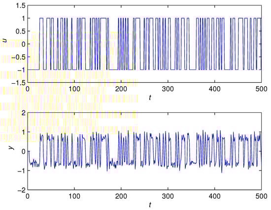
Figure 1.
The simulated input-output data versus t.
Table 2.
The parameter estimates and their errors with .
Table 3.
The parameter estimates and their errors with .
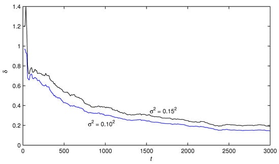
Figure 2.
The RGLS parameter estimation errors versus t with different variances.
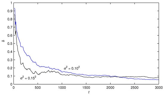
Figure 3.
The F-TS-RGLS parameter estimation errors versus t with different variances.
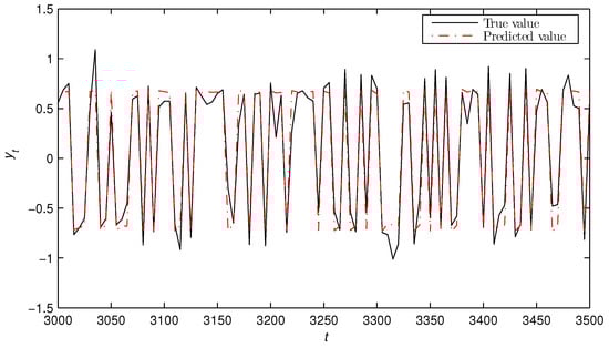
Figure 4.
The true outputs and the RGLS predicted outputs.
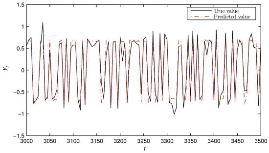
Figure 5.
The true outputs and the F-TS-RGLS predicted outputs.
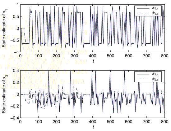
Figure 6.
State and its estimate versus t ().
From the simulation results in Table 2 and Table 3 and Figure 1, Figure 2, Figure 3, Figure 4, Figure 5 and Figure 6, we can draw the following conclusions.
- The estimation errors of the RGLS algorithm and the F-TS-RGLS algorithm became smaller with the data length increasing. This means that the proposed algorithms are effective.
- Under the same noise levels, the state estimator-based F-TS-RGLS algorithm could generate more accurate parameter estimates than the state estimator-based RGLS algorithm.
- The F-TS-RGLS algorithm could decrease the dimensions of the covariance matrices and improve the computational efficiency.
- The state estimates obtained from the bilinear state estimator could track their true values as t increased.
6. Conclusions
This paper presents a recursive parameter and state estimation algorithm on the basis of the hierarchical identification principle for bilinear systems. In this approach, the system parameters and states could be estimated interactively. The bilinear state estimator was derived based on the Kalman filter. Then, the state estimator-based RGLS algorithm and the state estimator-based F-TS-RGLS algorithm were proposed based on the data filtering technique and the decomposition-coordination principle. The simulation results showed that the state estimator-based F-TS-RGLS algorithm had higher parameter estimation accuracy compared with the state estimator-based RGLS algorithm. Moreover, the state estimator-based F-TS-RGLS algorithm could greatly improve the computational efficiency. The methods proposed in this paper could be combined the particle Monte Carlo methods [56,57] and some statistical methods to study the model selection and parameter estimation [58,59,60] for different systems [61,62,63,64,65,66] and could be applied to other fields [67,68,69,70,71,72] such as communication networks [73,74,75].
Author Contributions
Conceptualization and methodology, X.Z. and F.D.; software, X.Z. and L.X.; validation and analysis, A.A. and T.H. Finally, all the authors have read and approved the final manuscript.
Funding
This work was supported by the National Natural Science Foundation of China (No. 61873111), the 111 Project (B12018), and the Postgraduate Research and Practice Innovation Program of Jiangsu Province (KYCX18_1854).
Conflicts of Interest
The authors declare no conflict of interest.
References
- Zhang, K.; Jiang, B.; Shi, P. Adjustable parameter-based distributed fault estimation observer design for multiagent systems with directed graphs. IEEE Trans. Cybern. 2017, 47, 306–314. [Google Scholar] [CrossRef] [PubMed]
- Xu, L. A proportional differential control method for a time-delay system using the Taylor expansion approximation. Appl. Math. Comput. 2014, 236, 391–399. [Google Scholar] [CrossRef]
- Xu, L. Application of the Newton iteration algorithm to the parameter estimation for dynamical systems. J. Comput. Appl. Math. 2015, 288, 33–43. [Google Scholar] [CrossRef]
- Xu, L.; Chen, L.; Xiong, W.L. Parameter estimation and controller design for dynamic systems from the step responses based on the Newton iteration. Nonlinear Dyn. 2015, 79, 2155–2163. [Google Scholar] [CrossRef]
- Xu, L.; Ding, F. Parameter estimation for control systems based on impulse responses. Int. J. Control Autom. Syst. 2017, 15, 2471–2479. [Google Scholar] [CrossRef]
- Wen, Y.Z.; Yin, C.C. Solution of Hamilton-Jacobi-Bellman equation in optimal reinsurance strategy under dynamic VaR constraint. J. Funct. Spaces 2019, 2019, 6750892. [Google Scholar] [CrossRef]
- Xu, L. The parameter estimation algorithms based on the dynamical response measurement data. Adv. Mech. Eng. 2017, 9, 1–12. [Google Scholar] [CrossRef]
- Xu, L.; Ding, F. Iterative parameter estimation for signal models based on measured data. Circuits Syst. Signal Process. 2018, 37, 3046–3069. [Google Scholar] [CrossRef]
- Xu, L.; Xiong, W.L.; Alsaedi, A.; Hayat, T. Hierarchical parameter estimation for the frequency response based on the dynamical window data. Int. J. Control Autom. Syst. 2018, 16, 1756–1764. [Google Scholar] [CrossRef]
- Zhang, X.; Ding, F.; Xu, L.; Yang, E.F. Highly computationally efficient state filter based on the delta operator. Int. J. Adapt. Control Signal Process. 2019. [Google Scholar] [CrossRef]
- Chen, G.Y.; Gan, M.; Chen, C.L.P.; Li, H.X. A regularized variable projection algorithm for separable nonlinear least-squares problems. IEEE Trans. Autom. Control 2019, 64, 526–537. [Google Scholar] [CrossRef]
- Chen, G.Y.; Gan, M.; Ding, F.; Chen, C.L.P. Modified Gram-Schmidt method-based variable projection algorithm for separable nonlinear models. IEEE Trans. Neural Netw. Learn. Syst. 2019. [Google Scholar] [CrossRef]
- Gan, M.; Li, H.X. An efficient variable projection formulation for separable nonlinear least squares problems. IEEE Trans. Cybern. 2014, 44, 707–711. [Google Scholar] [CrossRef]
- Ding, F.; Liu, X.P.; Liu, G. Gradient based and least-squares based iterative identification methods for OE and OEMA systems. Digit. Signal Process. 2010, 20, 664–677. [Google Scholar] [CrossRef]
- Ding, F.; Liu, X.G.; Chu, J. Gradient-based and least-squares-based iterative algorithms for Hammerstein systems using the hierarchical identification principle. IET Control Theory Appl. 2013, 7, 176–184. [Google Scholar] [CrossRef]
- Ding, F. Decomposition based fast least squares algorithm for output error systems. Signal Process. 2013, 93, 1235–1242. [Google Scholar] [CrossRef]
- Ding, F. Two-stage least squares based iterative estimation algorithm for CARARMA system modeling. Appl. Math. Model. 2013, 37, 4798–4808. [Google Scholar] [CrossRef]
- Liu, Y.J.; Wang, D.Q.; Ding, F. Least squares based iterative algorithms for identifying Box-Jenkins models with finite measurement data. Digit. Signal Process. 2010, 20, 1458–1467. [Google Scholar] [CrossRef]
- Xu, H.; Ding, F.; Yang, E.F. Modeling a nonlinear process using the exponential autoregressive time series model. Nonlinear Dyn. 2019, 95, 2079–2092. [Google Scholar] [CrossRef]
- Liu, Q.Y.; Ding, F. Auxiliary model-based recursive generalized least squares algorithm for multivariate output-error autoregressive systems using the data filtering. Circuits Syst. Signal Process. 2019, 38, 590–610. [Google Scholar] [CrossRef]
- Ge, Z.W.; Ding, F.; Xu, L.; Alsaedi, A.; Hayat, T. Gradient-based iterative identification method for multivariate equation-error autoregressive moving average systems using the decomposition technique. J. Frankl. Inst. 2019, 356, 1658–1676. [Google Scholar] [CrossRef]
- Tian, X.P.; Niu, H.M. A bi-objective model with sequential search algorithm for optimizing network-wide train timetables. Comput. Ind. Eng. 2019, 127, 1259–1272. [Google Scholar] [CrossRef]
- Yang, F.; Zhang, P.; Li, X.X. The truncation method for the Cauchy problem of the inhomogeneous Helmholtz equation. Appl. Anal. 2019, 98, 991–1004. [Google Scholar] [CrossRef]
- Zhao, N.; Liu, R.; Chen, Y.; Wu, M.; Jiang, Y.; Xiong, W.; Liu, C. Contract design for relay incentive mechanism under dual asymmetric information in cooperative networks. Wirel. Netw. 2018, 24, 3029–3044. [Google Scholar] [CrossRef]
- Xu, G.H.; Shekofteh, Y.; Akgul, A.; Li, C.B.; Panahi, S. A new chaotic system with a self-excited attractor: Entropy measurement, signal encryption, and parameter estimation. Entropy 2018, 20, 86. [Google Scholar] [CrossRef]
- Li, X.Y.; Li, H.X.; Wu, B.Y. Piecewise reproducing kernel method for linear impulsive delay differential equations with piecewise constant arguments. Appl. Math. Comput. 2019, 349, 304–313. [Google Scholar] [CrossRef]
- Bruni, C.; Dipillo, G.; Koch, G. Bilinear systems: An appealing class of nearly linear systems in theory and applications. IEEE Trans. Autom. Control 1974, 19, 334–348. [Google Scholar] [CrossRef]
- Williamson, D. Observation of bilinear systems with application to biological control. Automatica 1977, 13, 243–254. [Google Scholar] [CrossRef]
- Yu, D.; Shields, D.N. A bilinear fault detection observer. Automatica 1996, 32, 1597–1602. [Google Scholar] [CrossRef]
- Mohler, R.R.; Kolodziej, W.J. An overview of bilinear system theory and applications. IEEE Trans. Syst. Man Cybern. 2007, 10, 683–688. [Google Scholar]
- Favoreel, W.; De Moor, B.; Van Overschee, P. Subspace identification of bilinear systems subject to white inputs. IEEE Trans. Autom. Control 1999, 44, 1157–1165. [Google Scholar] [CrossRef]
- Verdult, V.; Verhaegen, M. Identification of multivariable bilinear state space systems based on subspace techniques and separable least squares optimization. Int. J. Control 2001, 74, 1824–1836. [Google Scholar] [CrossRef]
- Larkowski, T.; Linden, J.G.; Vinsonneau, B.; Burnham, K.J. Frisch scheme identification for dynamic diagonal bilinear models. Int. J. Control 2009, 82, 1591–1604. [Google Scholar] [CrossRef]
- Hizir, N.B.; Phan, M.Q.; Betti, R.; Longman, R.W. Identification of discrete-time bilinear systems through equivalent linear models. Nonlinear Dyn. 2012, 69, 2065–2078. [Google Scholar]
- Vicario, F.; Phan, M.Q.; Betti, R.; Longman, R.W. Linear state representations for identification of bilinear discrete-time models by interaction matrices. Nonlinear Dyn. 2014, 77, 1561–1576. [Google Scholar] [CrossRef]
- Xu, L. The damping iterative parameter identification method for dynamical systems based on the sine signal measurement. Signal Process. 2016, 120, 660–667. [Google Scholar] [CrossRef]
- Xu, L.; Ding, F. Parameter estimation algorithms for dynamical response signals based on the multi-innovation theory and the hierarchical principle. IET Signal Process. 2017, 11, 228–237. [Google Scholar] [CrossRef]
- Xu, L.; Ding, F. Recursive least squares and multi-innovation stochastic gradient parameter estimation methods for signal modeling. Circuits Syst. Signal Process. 2017, 36, 1735–1753. [Google Scholar] [CrossRef]
- Gan, M.; Chen, C.L.P.; Chen, G.Y.; Chen, L. On some separated algorithms for separable nonlinear squares problems. IEEE Trans. Cybern. 2018, 48, 2866–2874. [Google Scholar] [CrossRef]
- Ding, F.; Liu, G.; Liu, X.P. Parameter estimation with scarce measurements. Automatica 2011, 47, 1646–1655. [Google Scholar] [CrossRef]
- Ding, F.; Liu, G.; Liu, X.P. Partially coupled stochastic gradient identification methods for non-uniformly sampled systems. IEEE Trans. Autom. Control 2010, 55, 1976–1981. [Google Scholar] [CrossRef]
- Zhao, S.Y.; Shmaliy, Y.S.; Ahn, C.K.; Liu, F. Adaptive-horizon iterative UFIR filtering algorithm with applications. IEEE Trans. Ind. Electron. 2018, 65, 6393–6402. [Google Scholar] [CrossRef]
- Zhao, S.Y.; Huang, B.; Liu, F. Linear optimal unbiased filter for time-variant systems without apriori information on initial conditions. IEEE Trans. Autom. Control 2017, 62, 882–887. [Google Scholar] [CrossRef]
- Xu, L.; Ding, F.; Gu, Y.; Alsaedi, A.; Hayat, T. A multi-innovation state and parameter estimation algorithm for a state space system with d-step state-delay. Signal Process. 2017, 140, 97–103. [Google Scholar] [CrossRef]
- Chopin, N.; Jacob, P.E.; Papaspiliopoulos, O. SMC2: An efficient algorithm for sequential analysis of state space models. J. R. Stat. Soc. Ser. B Stat. Methodol. 2013, 75, 397–426. [Google Scholar] [CrossRef]
- Van Wingerden, J.W.; Verhaegen, M. Subspace identification of bilinear and LPV systems for open-and closed-loop data. Automatica 2009, 45, 372–381. [Google Scholar] [CrossRef]
- Stroud, J.R.; Katzfuss, M.; Wikle, C.K. A Bayesian adaptive ensemble Kalman filter for sequential state and parameter estimation. Mon. Weather Rev. 2018, 46, 373–386. [Google Scholar] [CrossRef]
- Urteaga, I.; Bugallo, M.F.; Djurić, P.M. Sequential Monte Carlo methods under model uncertainty. In Proceedings of the 2016 IEEE Statistical Signal Processing Workshop (SSP), Palma de Mallorca, Spain, 26–29 June 2016. [Google Scholar]
- Martino, L.; Read, J.; Elvira, V.; Louzada, F. Cooperative parallel particle filters for online model selection and applications to urban mobility. Digit. Signal Process. 2017, 60, 172–185. [Google Scholar] [CrossRef]
- Schön, T.B.; Wills, A.; Ninness, B. System identification of nonlinear state-space models. Automatica 2011, 47, 39–49. [Google Scholar] [CrossRef]
- Li, M.H.; Liu, X.M. The least squares based iterative algorithms for parameter estimation of a bilinear system with autoregressive noise using the data filtering technique. Signal Process. 2018, 147, 23–34. [Google Scholar] [CrossRef]
- Phan, M.Q.; Vicario, F.; Longman, R.W.; Betti, R. Optimal bilinear observers for bilinear state-space models by interaction matrices. Int. J. Control 2015, 88, 1504–1522. [Google Scholar] [CrossRef]
- Zhang, X.; Ding, F.; Alsaadi, F.E.; Hayat, T. Recursive parameter identification of the dynamical models for bilinear state space systems. Nonlinear Dyn. 2017, 89, 2415–2429. [Google Scholar] [CrossRef]
- Zhang, X.; Ding, F.; Xu, L.; Yang, E.F. State filtering-based least squares parameter estimation for bilinear systems using the hierarchical identification principle. IET Control Theory Appl. 2018, 12, 1704–1713. [Google Scholar] [CrossRef]
- Zhang, X.; Xu, L.; Ding, F.; Hayat, T. Combined state and parameter estimation for a bilinear state space system with moving average noise. J. Frankl. Inst. 2018, 355, 3079–3103. [Google Scholar] [CrossRef]
- Martino, L.; Elvira, V.; Camps-Valls, G. Distributed Particle Metropolis-Hastings schemes. In Proceedings of the 2018 IEEE Statistical Signal Processing Workshop, Freiburg, Germany, 10–13 June 2018. [Google Scholar]
- Carvalho, C.M.; Johannes, M.S.; Lopes, H.F.; Polson, N.G. Particle learning and smoothing. Stat. Sci. 2010, 25, 88–106. [Google Scholar] [CrossRef]
- Ma, F.Y.; Yin, Y.K.; Li, M. Start-up process modelling of sediment microbial fuel cells based on data driven. Math. Probl. Eng. 2019, 2019, 7403732. [Google Scholar] [CrossRef]
- Pan, J.; Ma, H.; Jiang, X.; Ding, W.; Ding, F. Adaptive gradient-based iterative algorithm for multivariate controlled autoregressive moving average systems using the data filtering technique. Complexity 2018, 2018, 9598307. [Google Scholar] [CrossRef]
- Pan, J.; Li, W.; Zhang, H.P. Control algorithms of magnetic suspension systems based on the improved double exponential reaching law of sliding mode control. Int. J. Control Autom. Syst. 2018, 16, 2878–2887. [Google Scholar] [CrossRef]
- Wu, M.H.; Li, X.; Liu, C.; Liu, M.; Zhao, N.; Wang, J.; Wan, X.; Rao, Z.; Zhu, L. Robust global motion estimation for video security based on improved k-means clustering. J. Ambient Intell. Humaniz. Comput. 2019, 10, 439–448. [Google Scholar] [CrossRef]
- Wan, X.K.; Wu, H.; Qiao, F.; Li, F.C.; Li, Y.; Yan, Y.W.; Wei, J.X. Electrocardiogram baseline wander suppression based on the combination of morphological and wavelet transformation based filtering. Comput. Math. Methods Med. 2019, 2019, 7196156. [Google Scholar] [CrossRef]
- Wang, T.; Liu, L.; Zhang, J.; Schaeffer, E.; Wang, Y. A M-EKF fault detection strategy of insulation system for marine current turbine. Mech. Syst. Signal Process. 2019, 115, 269–280. [Google Scholar] [CrossRef]
- Wang, Y.; Si, Y.; Huang, B.; Lou, Z. Survey on the theoretical research and engineering applications of multivariate statistics process monitoring algorithms: 2008–2017. Can. J. Chem. Eng. 2018, 96, 2073–2085. [Google Scholar] [CrossRef]
- Gu, Y.; Chou, Y.; Liu, J.; Ji, Y. Moving horizon estimation for multirate systems with time-varying time-delays. J. Frankl. Inst. 2019, 356, 2325–2345. [Google Scholar] [CrossRef]
- Wang, Y.J.; Ding, F. Iterative estimation for a non-linear IIR filter with moving average noise by means of the data filtering technique. IMA J. Math. Control Inf. 2017, 34, 745–764. [Google Scholar] [CrossRef]
- Cao, Y.; Lu, H.; Wen, T. A safety computer system based on multi-sensor data processing. Sensors 2019, 19, 818. [Google Scholar] [CrossRef]
- Cao, Y.; Zhang, Y.; Wen, T.; Li, P. Research on dynamic nonlinear input prediction of fault diagnosis based on fractional differential operator equation in high-speed train control system. Chaos 2019, 29, 013130. [Google Scholar] [CrossRef]
- Cao, Y.; Li, P.; Zhang, Y. Parallel processing algorithm for railway signal fault diagnosis data based on cloud computing. Future Gener. Comput. Syst. 2018, 88, 279–283. [Google Scholar] [CrossRef]
- Cao, Y.; Ma, L.C.; Xiao, S.; Zhang, X.; Xu, W. Standard analysis for transfer delay in CTCS-3. Chin. J. Electron. 2017, 26, 1057–1063. [Google Scholar] [CrossRef]
- Jiang, C.M.; Zhang, F.F.; Li, T.X. Synchronization and antisynchronization of N-coupled fractional-order complex chaotic systems with ring connection. Math. Methods Appl. Sci. 2018, 41, 2625–2638. [Google Scholar] [CrossRef]
- Zhang, W.H.; Xue, L.; Jiang, X. Global stabilization for a class of stochastic nonlinear systems with SISS-like conditions and time delay. Int. J. Robust Nonlinear Control 2018, 28, 3909–3926. [Google Scholar] [CrossRef]
- Zhao, N.; Chen, Y.; Liu, R.; Wu, M.H.; Xiong, W. Monitoring strategy for relay incentive mechanism in cooperative communication networks. Comput. Electr. Eng. 2017, 60, 14–29. [Google Scholar] [CrossRef]
- Zhao, N.; Wu, M.H.; Chen, J.J. Android-based mobile educational platform for speech signal processing. Int. J. Electr. Eng. Edu. 2017, 54, 3–16. [Google Scholar] [CrossRef]
- Ji, Y.; Ding, F. Multiperiodicity and exponential attractivity of neural networks with mixed delays. Circuits Syst. Signal Process. 2017, 36, 2558–2573. [Google Scholar] [CrossRef]


© 2019 by the authors. Licensee MDPI, Basel, Switzerland. This article is an open access article distributed under the terms and conditions of the Creative Commons Attribution (CC BY) license (http://creativecommons.org/licenses/by/4.0/).