Optimal Fourth, Eighth and Sixteenth Order Methods by Using Divided Difference Techniques and Their Basins of Attraction and Its Application

Abstract

The principal objective of this work is to propose a fourth, eighth and sixteenth order scheme for solving a nonlinear equation. In terms of computational cost, per iteration, the fourth order method uses two evaluations of the function and one evaluation of the first derivative; the eighth order method uses three evaluations of the function and one evaluation of the first derivative; and sixteenth order method uses four evaluations of the function and one evaluation of the first derivative. So these all the methods have satisfied the Kung-Traub optimality conjecture. In addition, the theoretical convergence properties of our schemes are fully explored with the help of the main theorem that demonstrates the convergence order. The performance and effectiveness of our optimal iteration functions are compared with the existing competitors on some standard academic problems. The conjugacy maps of the presented method and other existing eighth order methods are discussed, and their basins of attraction are also given to demonstrate their dynamical behavior in the complex plane. We apply the new scheme to find the optimal launch angle in a projectile motion problem and Planck’s radiation law problem as an application.

1. Introduction

One of the most frequent problems in engineering, scientific computing and applied mathematics, in general, is the problem of solving a nonlinear equation $f\left(x\right)=0$. In most of the cases, whenever real problems are faced, such as weather forecasting, accurate positioning of satellite systems in the desired orbit, measurement of earthquake magnitudes and other high-level engineering problems, only approximate solutions may get resolved. However, only in rare cases, it is possible to solve the governing equations exactly. The most familiar method of solving non linear equation is Newton’s iteration method. The local order of convergence of Newton’s method is two and it is an optimal method with two function evaluations per iterative step.

In the past decade, several higher order iterative methods have been developed and analyzed for solving nonlinear equations that improve classical methods such as Newton’s method, Chebyshev method, Halley’s iteration method, etc. As the order of convergence increases, so does the number of function evaluations per step. Hence, a new index to determine the efficiency called the efficiency index is introduced in [1] to measure the balance between these quantities. Kung-Traub [2] conjectured that the order of convergence of any multi-point without memory method with d function evaluations cannot exceed the bound $2^{d-1}$, the optimal order. Thus the optimal order for three evaluations per iteration would be four, four evaluations per iteration would be eight, and so on. Recently, some fourth and eighth order optimal iterative methods have been developed (see [3,4,5,6,7,8,9,10,11,12,13,14] and references therein). A more extensive list of references as well as a survey on the progress made in the class of multi-point methods is found in the recent book by Petkovic et al. [11].

This paper is organized as follows. An optimal fourth, eighth and sixteenth order methods are developed by using divided difference techniques in Section 2. In Section 3, convergence order is analyzed. In Section 4, tested numerical examples to compare the proposed methods with other known optimal methods. The problem of Projectile motion is discussed in Section 5 where the presented methods are applied on this problem with some existing ones. In Section 6, we obtain the conjugacy maps of these methods to make a comparison from dynamical point of view. In Section 7, the proposed methods are studied in the complex plane using basins of attraction. Section 8 gives concluding remarks.

2. Design of an Optimal Fourth, Eighth and Sixteenth Order Methods

Definition 1

([15]). If the sequence $\left\{x_n\right\}$ tends to a limit $x^{\ast }$ in such a way that

$$\underset{n\to \infty }{lim}\frac{x_{n+1}-x^{\ast }}{{(x_n-x^{\ast })}^p}=C$$

for $p\ge 1$, then the order of convergence of the sequence is said to be p, and C is known as the asymptotic error constant. If $p=1$, $p=2$ or $p=3$, the convergence is said to be linear, quadratic or cubic, respectively.

Let $e_n=x_n-x^{\ast }$, then the relation

$$e_{n+1}=C{e}_n^p+O\left(e_n^{p+1}\right)=O\left(e_n^p\right).$$

(1)

is called the error equation. The value of p is called the order of convergence of the method.

Definition 2

([1]). The Efficiency Index is given by

$$EI=p^{\frac{1}{d}},$$

(2)

where d is the total number of new function evaluations (the values of f and its derivatives) per iteration.

Let $x_{n+1}=\psi \left(x_n\right)$ define an Iterative Function (IF). Let $x_{n+1}$ be determined by new information at $x_n,{\varphi }_1\left(x_n\right),...,{\varphi }_{\mathrm{i}}\left(x_n\right),\mathrm{i}\ge 1$. No old information is reused. Thus,

$$x_{n+1}=\psi (x_n,{\varphi }_1\left(x_n\right),...,{\varphi }_{\mathrm{i}}\left(x_n\right)).$$

(3)

Then $\psi$ is called a multipoint IF without memory.

The Newton (also called Newton-Raphson) IF (2^ndNR) is given by

$${\psi }_{2^{nd}NR}\left(x\right)=x-\frac{f\left(x\right)}{f^{\prime }\left(x\right)}.$$

(4)

The 2^ndNR IF is one-point IF with two function evaluations and it satisfies the Kung-Traub conjecture with $d=2$. Further, $E{I}_{2^{nd}NR}=1.414$.

2.1. An Optimal Fourth Order Method

We attempt to get a new optimal fourth order IF as follows, let us consider two step Newton’s method

$${\psi }_{4^{th}NR}\left(x\right)={\psi }_{2^{nd}NR}\left(x\right)-\frac{f\left({\psi }_{2^{nd}NR}\left(x\right)\right)}{f^{\prime }\left({\psi }_{2^{nd}NR}\left(x\right)\right)}.$$

(5)

The above one is having fourth order convergence with four function evaluations. But, this is not an optimal method. To get an optimal, need to reduce a function and preserve the same convergence order, and so we estimate $f^{\prime }\left({\psi }_{2^{nd}NR}\left(x\right)\right)$ by the following polynomial

$$q\left(t\right)=a_0+a_1(t-x)+a_2{(t-x)}^2,$$

(6)

which satisfies

$$q\left(x\right)=f\left(x\right),q^{\prime }\left(x\right)=f^{\prime }\left(x\right),q\left({\psi }_{2^{nd}NR}\left(x\right)\right)=f\left({\psi }_{2^{nd}NR}\left(x\right)\right).$$

On implementing the above conditions on Equation (6), we obtain three unknowns $a_0$, $a_1$ and $a_2$. Let us define the divided differences

$$f[y,x]=\frac{f\left(y\right)-f\left(x\right)}{y-x},f[y,x,x]=\frac{f[y,x]-f^{\prime }\left(x\right)}{y-x}.$$

From conditions, we get $a_0=f\left(x\right)$, $a_1=f^{\prime }\left(x\right)$ and $a_2=f[{\psi }_{2^{nd}NR}\left(x\right),x,x]$, respectively, by using divided difference techniques. Now, we have the estimation

$$\begin{array}{c}\hfill f^{\prime }\left({\psi }_{2^{nd}NR}\left(x\right)\right)\approx q^{\prime }\left({\psi }_{2^{nd}NR}\left(x\right)\right)=a_1+2a_2({\psi }_{2^{th}NR}\left(x\right)-x).\end{array}$$

Finally, we propose a new optimal fourth order method as

$${\psi }_{4^{th}YM}\left(x\right)={\psi }_{2^{nd}NR}\left(x\right)-\frac{f\left({\psi }_{2^{nd}NR}\left(x\right)\right)}{f^{\prime }\left(x\right)+2f[{\psi }_{2^{nd}NR}\left(x\right),x,x]({\psi }_{2^{th}NR}\left(x\right)-x)}.$$

(7)

The efficiency of the method (7) is $E{I}_{4thYM}=1.587$.

2.2. An Optimal Eighth Order Method

Next, we attempt to get a new optimal eighth order IF as following way

$${\psi }_{8^{th}YM}\left(x\right)={\psi }_{4^{th}YM}\left(x\right)-\frac{f\left({\psi }_{4^{th}YM}\left(x\right)\right)}{f^{\prime }\left({\psi }_{4^{th}YM}\left(x\right)\right)}.$$

The above one is having eighth order convergence with five function evaluations. But, this is not an optimal method. To get an optimal, need to reduce a function and preserve the same convergence order, and so we estimate $f^{\prime }\left({\psi }_{4^{th}YM}\left(x\right)\right)$ by the following polynomial

$$q\left(t\right)=b_0+b_1(t-x)+b_2{(t-x)}^2+b_3{(t-x)}^3,$$

(8)

which satisfies

$$q\left(x\right)=f\left(x\right),q^{\prime }\left(x\right)=f^{\prime }\left(x\right),q\left({\psi }_{2^{nd}NR}\left(x\right)\right)=f\left({\psi }_{2^{nd}NR}\left(x\right)\right),q\left({\psi }_{4^{th}YM}\left(x\right)\right)=f\left({\psi }_{4^{th}YM}\left(x\right)\right).$$

On implementing the above conditions on (8), we obtain four linear equations with four unknowns $b_0$, $b_1$, $b_2$ and $b_3$. From conditions, we get $b_0=f\left(x\right)$ and $b_1=f^{\prime }\left(x\right)$. To find $b_2$ and $b_3$, we solve the following equations:

$$\begin{array}{ccc}\hfill f\left({\psi }_{2^{nd}NR}\left(x\right)\right)& =& f\left(x\right)+f^{\prime }\left(x\right)({\psi }_{2^{nd}NR}\left(x\right)-x)+b_2{({\psi }_{2^{nd}NR}\left(x\right)-x)}^2+b_3{({\psi }_{2^{nd}NR}\left(x\right)-x)}^3\hfill \\ \hfill f\left({\psi }_{4^{th}YM}\left(x\right)\right)& =& f\left(x\right)+f^{\prime }\left(x\right)({\psi }_{4^{th}YM}\left(x\right)-x)+b_2{({\psi }_{4^{th}YM}\left(x\right)-x)}^2+b_3{({\psi }_{4^{th}YM}\left(x\right)-x)}^3.\hfill \end{array}$$

Thus by applying divided differences, the above equations simplifies to

$$\begin{array}{cc}\hfill b_2+b_3({\psi }_{2^{nd}NR}\left(x\right)-x)& =f[{\psi }_{2^{nd}NR}\left(x\right),x,x]\end{array}$$

(9)

$$\begin{array}{cc}\hfill b_2+b_3({\psi }_{4^{th}YM}\left(x\right)-x)& =f[{\psi }_{4^{th}YM}\left(x\right),x,x]\end{array}$$

(10)

Solving Equations (9) and (14), we have

$$\begin{array}{cc}{b}_2\hfill & =\frac{f[{\psi }_{2^{nd}NR}\left(x\right),x,x]({\psi }_{4^{th}PM}\left(x\right)-x)-f[{\psi }_{4^{th}YM}\left(x\right),x,x]({\psi }_{2^{nd}NR}\left(x\right)-x)}{{\psi }_{4^{th}YM}\left(x\right)-{\psi }_{2^{nd}NR}\left(x\right)},\hfill \\ b_3\hfill & =\frac{f[{\psi }_{4^{th}YM}\left(x\right),x,x]-f[{\psi }_{2^{nd}NR}\left(x\right),x,x]}{{\psi }_{4^{th}YM}\left(x\right)-{\psi }_{2^{nd}NR}\left(x\right)}.\hfill \end{array}$$

(11)

Further, using Equation (11), we have the estimation

$$\begin{array}{c}{f}^{\prime }\left({\psi }_{4^{th}YM}\left(x\right)\right)\approx q^{\prime }\left({\psi }_{4^{th}YM}\left(x\right)\right)=b_1+2b_2({\psi }_{4^{th}YM}\left(x\right)-x)+3b_3{({\psi }_{4^{th}YM}\left(x\right)-x)}^2.\hfill \end{array}$$

Finally, we propose a new optimal eighth order method as

$$\begin{array}{c}{\psi }_{8^{th}YM}\left(x\right)={\psi }_{4^{th}YM}\left(x\right)-\frac{f\left({\psi }_{4^{th}YM}\left(x\right)\right)}{f^{\prime }\left(x\right)+2b_2({\psi }_{4^{th}YM}\left(x\right)-x)+3b_3{({\psi }_{4^{th}YM}\left(x\right)-x)}^2}.\hfill \end{array}$$

(12)

The efficiency of the method (12) is $E{I}_{8thYM}=1.682$. Remark that the method is seems a particular case of the method of Khan et al. [16], they used weight function to develop their methods. Whereas we used finite difference scheme to develop proposed methods. We can say the methods $4^{th}YM$ and $8^{th}YM$ are reconstructed of Khan et al. [16] methods.

2.3. An Optimal Sixteenth Order Method

Next, we attempt to get a new optimal sixteenth order IF as following way

$${\psi }_{{16}^{th}YM}\left(x\right)={\psi }_{8^{th}YM}\left(x\right)-\frac{f\left({\psi }_{8^{th}YM}\left(x\right)\right)}{f^{\prime }\left({\psi }_{8^{th}YM}\left(x\right)\right)}.$$

The above one is having eighth order convergence with five function evaluations. However, this is not an optimal method. To get an optimal, need to reduce a function and preserve the same convergence order, and so we estimate $f^{\prime }\left({\psi }_{8^{th}YM}\left(x\right)\right)$ by the following polynomial

$$q\left(t\right)=c_0+c_1(t-x)+c_2{(t-x)}^2+c_3{(t-x)}^3+c_4{(t-x)}^4,$$

(13)

which satisfies

$$\begin{array}{c}\hfill q\left(x\right)=f\left(x\right),q^{\prime }\left(x\right)=f^{\prime }\left(x\right),q\left({\psi }_{2^{nd}NR}\left(x\right)\right)=f\left({\psi }_{2^{nd}NR}\left(x\right)\right),\\ \hfill q\left({\psi }_{4^{th}YM}\left(x\right)\right)=f\left({\psi }_{4^{th}YM}\left(x\right)\right),q\left({\psi }_{8^{th}YM}\left(x\right)\right)=f\left({\psi }_{8^{th}YM}\left(x\right)\right).\end{array}$$

On implementing the above conditions on (13), we obtain four linear equations with four unknowns $c_0$, $c_1$, $c_2$ and $c_3$. From conditions, we get $c_0=f\left(x\right)$ and $c_1=f^{\prime }\left(x\right)$. To find $c_2$, $c_3$ and $c_4$, we solve the following equations:

$$\begin{array}{cc}f\left({\psi }_{2^{nd}NR}\left(x\right)\right)=& f\left(x\right)+f^{\prime }\left(x\right)({\psi }_{2^{nd}NR}\left(x\right)-x)+c_2{({\psi }_{2^{nd}NR}\left(x\right)-x)}^2+c_3{({\psi }_{2^{nd}NR}\left(x\right)-x)}^3+c_4{({\psi }_{2^{nd}NR}\left(x\right)-x)}^4\\ f\left({\psi }_{4^{th}YM}\left(x\right)\right)=& f\left(x\right)+f^{\prime }\left(x\right)({\psi }_{4^{th}YM}\left(x\right)-x)+c_2{({\psi }_{4^{th}YM}\left(x\right)-x)}^2+c_3{({\psi }_{4^{th}YM}\left(x\right)-x)}^3+c_4{({\psi }_{4^{th}YM}\left(x\right)-x)}^4\\ f\left({\psi }_{8^{th}YM}\left(x\right)\right)=& f\left(x\right)+f^{\prime }\left(x\right)({\psi }_{8^{th}YM}\left(x\right)-x)+c_2{({\psi }_{8^{th}YM}\left(x\right)-x)}^2+c_3{({\psi }_{8^{th}YM}\left(x\right)-x)}^3+c_4{({\psi }_{8^{th}YM}\left(x\right)-x)}^4.\end{array}$$

Thus by applying divided differences, the above equations simplifies to

$$\begin{array}{cc}\hfill c_2+c_3({\psi }_{2^{nd}NR}\left(x\right)-x)+c_4{({\psi }_{2^{nd}NR}\left(x\right)-x)}^2& =f[{\psi }_{2^{nd}NR}\left(x\right),x,x]\\ \hfill c_2+c_3({\psi }_{4^{th}YM}\left(x\right)-x)+c_4{({\psi }_{4^{th}YM}\left(x\right)-x)}^2& =f[{\psi }_{4^{th}YM}\left(x\right),x,x]\\ \hfill c_2+c_3({\psi }_{8^{th}YM}\left(x\right)-x)+c_4{({\psi }_{8^{th}YM}\left(x\right)-x)}^2& =f[{\psi }_{8^{th}YM}\left(x\right),x,x]\end{array}$$

(14)

Solving Equation (14), we have

$$\begin{array}{cc}\hfill c_2& =\frac{\left(f[{\psi }_{2^{nd}NR}\left(x\right),x,x]\left(-S_2^2{S}_3+S_2{S}_3^2\right)+f[{\psi }_{4^{th}YM}\left(x\right),x,x]\left(S_1^2{S}_3-S_1{S}_3^2\right)+f[{\psi }_{8^{th}YM}\left(x\right),x,x]\left(-S_1^2{S}_2+S_1{S}_2^2\right)\right)}{-S_1^2{S}_2+S_1{S}_2^2+S_1^2{S}_3-S_2^2{S}_3-S_1{S}_3^2+S_2{S}_3^2},\hfill \\ \hfill c_3& =\frac{\left(f[{\psi }_{2^{nd}NR}\left(x\right),x,x]\left(S_2^2-S_3^2\right)+f[{\psi }_{4^{th}YM}\left(x\right),x,x]\left(-S_1^2+S_3^2\right)+f[{\psi }_{8^{th}YM}\left(x\right),x,x]\left(S_1^2-S_2^2\right)\right)}{-S_1^2{S}_2+S_1{S}_2^2+S_1^2{S}_3-S_2^2{S}_3-S_1{S}_3^2+S_2{S}_3^2},\hfill \\ \hfill c_4& =\frac{\left(f[{\psi }_{2^{nd}NR}\left(x\right),x,x]\left(-S_2+S_3\right)+f[{\psi }_{4^{th}YM}\left(x\right),x,x]\left(S_1-S_3\right)+f[{\psi }_{8^{th}YM}\left(x\right),x,x]\left(-S_1+S_2\right)\right)}{-S_1^2{S}_2+S_1{S}_2^2+S_1^2{S}_3-S_2^2{S}_3-S_1{S}_3^2+S_2{S}_3^2},\hfill \\ \hfill S_1& ={\psi }_{2^{nd}NR}\left(x\right)-x,S_2={\psi }_{4^{th}YM}\left(x\right)-x,S_3={\psi }_{8^{th}YM}\left(x\right)-x.\hfill \end{array}$$

(15)

Further, using Equation (15), we have the estimation

$$\begin{array}{c}{f}^{\prime }\left({\psi }_{8^{th}YM}\left(x\right)\right)\approx q^{\prime }\left({\psi }_{8^{th}YM}\left(x\right)\right)=c_1+2c_2({\psi }_{8^{th}YM}\left(x\right)-x)+3c_3{({\psi }_{8^{th}YM}\left(x\right)-x)}^2+4c_4{({\psi }_{8^{th}YM}\left(x\right)-x)}^3.\hfill \end{array}$$

Finally, we propose a new optimal sixteenth order method as

$$\begin{array}{c}{\psi }_{{16}^{th}YM}\left(x\right)={\psi }_{8^{th}YM}\left(x\right)-\frac{f\left({\psi }_{8^{th}YM}\left(x\right)\right)}{f^{\prime }\left(x\right)+2c_2({\psi }_{8^{th}YM}\left(x\right)-x)+3c_3{({\psi }_{8^{th}YM}\left(x\right)-x)}^2+4c_4{({\psi }_{8^{th}YM}\left(x\right)-x)}^3}.\hfill \end{array}$$

(16)

The efficiency of the method (16) is $E{I}_{16thYM}=1.741$.

3. Convergence Analysis

In this section, we prove the convergence analysis of proposed $IFs$ with help of Mathematica software.

Theorem 1.

Let $f:D\subset \mathbb{R}\to \mathbb{R}$ be a sufficiently smooth function having continuous derivatives. If $f\left(x\right)$ has a simple root $x^{\ast }$ in the open interval D and $x_0$ chosen in sufficiently small neighborhood of $x^{\ast }$, then the method$4^{th}YM$IFs (7) is of local fourth order convergence, and the$8^{th}YM$IFs (12) is of local eighth order convergence.

Proof. 

Let $e=x-x^{\ast }$ and ${\displaystyle c\left[j\right]=\frac{f^{\left(j\right)}\left(x^{\ast }\right)}{j!f^{\prime }\left(x^{\ast }\right)},j=2,3,4,...}$. Expanding $f\left(x\right)$ and $f^{\prime }\left(x\right)$ about $x^{\ast }$ by Taylor’s method, we have

$$f\left(x\right)=f^{\prime }\left(x^{\ast }\right)\left(e+e^{2}c\left[2\right]+e^{3}c\left[3\right]+e^{4}c\left[4\right]+e^{5}c\left[5\right]+e^{6}c\left[6\right]+e^{7}c\left[7\right]+e^{8}c\left[8\right]+\dots \right)$$

(17)

and

$$\begin{array}{c}{f}^{\prime }\left(x\right)=f^{\prime }\left(x^{\ast }\right)\left(1+2ec\left[2\right]+3e^{2}c\left[3\right]+4e^{3}c\left[4\right]+5e^{4}c\left[5\right]+6e^{5}c\left[6\right]+7e^{6}c\left[7\right]+8e^{7}c\left[8\right]+9e^{8}c\left[9\right]+\dots \right)\end{array}$$

(18)

Thus,

$$\begin{array}{c}{\psi }_{2^{nd}NR}\left(x\right)=x^{\ast }+c\left[2\right]e^2+\left(-2c{\left[2\right]}^2+2c\left[3\right]\right)e^3+\left(4c{\left[2\right]}^3-7c\left[2\right]c\left[3\right]+3c\left[4\right]\right)e^4+(-8c{\left[2\right]}^4\hfill \\ +20c{\left[2\right]}^{2}c\left[3\right]-6c{\left[3\right]}^2-10c\left[2\right]c\left[4\right]+4c\left[5\right])e^5+(16c{\left[2\right]}^5-52c{\left[2\right]}^{3}c\left[3\right]+28c{\left[2\right]}^{2}c\left[4\right]-17c\left[3\right]c\left[4\right]\hfill \\ +c\left[2\right](33c{\left[3\right]}^2-13c\left[5\right])+5c\left[6\right])e^6-2(16c{\left[2\right]}^6-64c{\left[2\right]}^{4}c\left[3\right]-9c{\left[3\right]}^3+36c{\left[2\right]}^{3}c\left[4\right]+6c{\left[4\right]}^2+9c{\left[2\right]}^2{(7c\left[3\right]}^2\hfill \\ -2c\left[5\right])+11c\left[3\right]c\left[5\right]+c\left[2\right](-46c\left[3\right]c\left[4\right]+8c\left[6\right])-3c\left[7\right])e^7+(64c{\left[2\right]}^7-304c{\left[2\right]}^{5}c\left[3\right]\hfill \\ +176c{\left[2\right]}^{4}c\left[4\right]+75c{\left[3\right]}^{2}c\left[4\right]+c{\left[2\right]}^3(408c{\left[3\right]}^2-92c\left[5\right])-31c\left[4\right]c\left[5\right]-27c\left[3\right]c\left[6\right]\hfill \\ +c{\left[2\right]}^2(-348c\left[3\right]c\left[4\right]+44c\left[6\right])+c\left[2\right](-135c{\left[3\right]}^3+64c{\left[4\right]}^2+118c\left[3\right]c\left[5\right]-19c\left[7\right])+7c\left[8\right])e^8+\dots .\hfill \end{array}$$

(19)

Expanding $f\left({\psi }_{2^{nd}NR}\left(x\right)\right)$ about $x^{\ast }$ by Taylor’s method, we have

$$\begin{array}{c}f\left({\psi }_{2^{nd}NR}\left(x\right)\right)=f^{\prime }\left(x^{\ast }\right)(c\left[2\right]e^2+\left(-2c{\left[2\right]}^2+2c\left[3\right]\right)e^3+\left(5c{\left[2\right]}^3-7c\left[2\right]c\left[3\right]+3c\left[4\right]\right)e^4-2(6c{\left[2\right]}^4\hfill \\ -12c{\left[2\right]}^{2}c\left[3\right]+3c{\left[3\right]}^2+5c\left[2\right]c\left[4\right]-2c\left[5\right])e^5+(28c{\left[2\right]}^5-73c{\left[2\right]}^{3}c\left[3\right]+34c{\left[2\right]}^{2}c\left[4\right]-17c\left[3\right]c\left[4\right]\hfill \\ +c\left[2\right](37c{\left[3\right]}^2-13c\left[5\right])+5c\left[6\right])e^6-2(32c{\left[2\right]}^6-103c{\left[2\right]}^{4}c\left[3\right]-9c{\left[3\right]}^3+52c{\left[2\right]}^{3}c\left[4\right]+6c{\left[4\right]}^2\hfill \\ +c{\left[2\right]}^2(80c{\left[3\right]}^2-22c\left[5\right])+11c\left[3\right]c\left[5\right]+c\left[2\right](-52c\left[3\right]c\left[4\right]+8c\left[6\right])-3c\left[7\right])e^7\hfill \\ +(144c{\left[2\right]}^7-552c{\left[2\right]}^{5}c\left[3\right]+297c{\left[2\right]}^{4}c\left[4\right]+75c{\left[3\right]}^{2}c\left[4\right]+2c{\left[2\right]}^3(291c{\left[3\right]}^2-67c\left[5\right])\hfill \\ -31c\left[4\right]c\left[5\right]-27c\left[3\right]c\left[6\right]+c{\left[2\right]}^2{(-455c\left[3\right]c\left[4\right]+54c\left[6\right])+c\left[2\right](-147c\left[3\right]}^3+73c{\left[4\right]}^2\hfill \\ +134c\left[3\right]c\left[5\right]-19c\left[7\right])+7c\left[8\right])e^8+\dots .)\hfill \end{array}$$

(20)

Using Equations (17)–(20) in divided difference techniques. We have

$$\begin{array}{c}f[{\psi }_{2^{nd}NR}\left(x\right),x,x]=f^{\prime }\left(x^{\ast }\right)(c\left[2\right]+2c\left[3\right]e+\left(c\left[2\right]c\left[3\right]+3c\left[4\right]\right)e^2+2(-c{\left[2\right]}^{2}c\left[3\right]+c{\left[3\right]}^2\hfill \\ +c\left[2\right]c\left[4\right]+2c\left[5\right])e^3+\left(4c{\left[2\right]}^{3}c\left[3\right]-3c{\left[2\right]}^{2}c\left[4\right]+7c\left[3\right]c\left[4\right]+c\left[2\right](-7c{\left[3\right]}^2+3c\left[5\right])+5c\left[6\right]\right)e^4\hfill \\ +(-8c{\left[2\right]}^{4}c\left[3\right]-6c{\left[3\right]}^3+4c{\left[2\right]}^{3}c\left[4\right]+4c{\left[2\right]}^2(5c{\left[3\right]}^2-c\left[5\right])+10c\left[3\right]c\left[5\right]\hfill \\ +4c\left[2\right](-5c\left[3\right]c\left[4\right]+c\left[6\right])+6(c{\left[4\right]}^2+c\left[7\right]))e^5+(16c{\left[2\right]}^{5}c\left[3\right]-4c{\left[2\right]}^{4}c\left[4\right]\hfill \\ -25c{\left[3\right]}^{2}c\left[4\right]+17c\left[4\right]c\left[5\right]+c{\left[2\right]}^3(-52c{\left[3\right]}^2+5c\left[5\right])+c{\left[2\right]}^2(46c\left[3\right]c\left[4\right]-5c\left[6\right])\hfill \\ +13c\left[3\right]c\left[6\right]+c\left[2\right](33c{\left[3\right]}^3-14c{\left[4\right]}^2-26c\left[3\right]c\left[5\right]+5c\left[7\right])+7c\left[8\right])e^6+\dots .)\hfill \end{array}$$

(21)

Substituting Equations (18)–(21) into Equation (7), we obtain, after simplifications,

$$\begin{array}{cc}{\psi }_{4^{th}YM}\left(x\right)\hfill & =x^{\ast }+\left(c{\left[2\right]}^3-c\left[2\right]c\left[3\right]\right)e^4-2\left(2c{\left[2\right]}^4-4c{\left[2\right]}^{2}c\left[3\right]+c{\left[3\right]}^2+c\left[2\right]c\left[4\right]\right)e^5+(10c{\left[2\right]}^5-30c{\left[2\right]}^{3}c\left[3\right]\hfill \\ & +12c{\left[2\right]}^{2}c\left[4\right]-7c\left[3\right]c\left[4\right]+3c\left[2\right](6c{\left[3\right]}^2-c\left[5\right]))e^6-2(10c{\left[2\right]}^6-40c{\left[2\right]}^{4}c\left[3\right]-6c{\left[3\right]}^3\hfill \\ & +20c{\left[2\right]}^{3}c\left[4\right]+3c{\left[4\right]}^2+8c{\left[2\right]}^2(5c{\left[3\right]}^2-c\left[5\right])+5c\left[3\right]c\left[5\right]+c\left[2\right](-26c\left[3\right]c\left[4\right]+2c\left[6\right]))e^7+(36c{\left[2\right]}^7\hfill \\ & -178c{\left[2\right]}^{5}c\left[3\right]+101c{\left[2\right]}^{4}c\left[4\right]+50c{\left[3\right]}^{2}c\left[4\right]+3c{\left[2\right]}^3(84c{\left[3\right]}^2-17c\left[5\right])-17c\left[4\right]c\left[5\right]-13c\left[3\right]c\left[6\right]\hfill \\ & +c{\left[2\right]}^2(-209c\left[3\right]c\left[4\right]+20c\left[6\right])+c\left[2\right](-91c{\left[3\right]}^3+37c{\left[4\right]}^2+68c\left[3\right]c\left[5\right]-5c\left[7\right]))e^8+\dots .\hfill \end{array}$$

(22)

Expanding $f\left({\psi }_{4^{th}YM}\left(x\right)\right)$ about $x^{\ast }$ by Taylor’s method, we have

$$\begin{array}{cc}f\left({\psi }_{4^{th}YM}\left(x\right)\right)\hfill & =f^{\prime }\left(x^{\ast }\right)(\left(c{\left[2\right]}^3-c\left[2\right]c\left[3\right]\right)e^4-2\left(2c{\left[2\right]}^4-4c{\left[2\right]}^{2}c\left[3\right]+c{\left[3\right]}^2+c\left[2\right]c\left[4\right]\right)e^5+(10c{\left[2\right]}^5\hfill \\ & -30c{\left[2\right]}^{3}c\left[3\right]+12c{\left[2\right]}^{2}c\left[4\right]-7c\left[3\right]c\left[4\right]+3c\left[2\right](6c{\left[3\right]}^2-c\left[5\right]))e^6-2(10c{\left[2\right]}^6-40c{\left[2\right]}^{4}c\left[3\right]\hfill \\ & -6c{\left[3\right]}^3+20c{\left[2\right]}^{3}c\left[4\right]+3c{\left[4\right]}^2+8c{\left[2\right]}^2(5c{\left[3\right]}^2-c\left[5\right])+5c\left[3\right]c\left[5\right]+c\left[2\right](-26c\left[3\right]c\left[4\right]+2c\left[6\right]))e^7\hfill \\ & +(37c{\left[2\right]}^7-180c{\left[2\right]}^{5}c\left[3\right]+101c{\left[2\right]}^{4}c\left[4\right]+50c{\left[3\right]}^{2}c\left[4\right]+c{\left[2\right]}^3(253c{\left[3\right]}^2-51c\left[5\right])-17c\left[4\right]c\left[5\right]\hfill \\ & -13c\left[3\right]c\left[6\right]+c{\left[2\right]}^2(-209c\left[3\right]c\left[4\right]+20c\left[6\right])+c\left[2\right](-91c{\left[3\right]}^3+37c{\left[4\right]}^2+68c\left[3\right]c\left[5\right]-5c\left[7\right]))e^8+\dots .)\hfill \end{array}$$

(23)

Now,

$$\begin{array}{cc}f[{\psi }_{4^{th}YM}\left(x\right),x,x]\hfill & =f^{\prime }\left(x^{\ast }\right)(c\left[2\right]+2c\left[3\right]e+3c\left[4\right]e^2+4c\left[5\right]e^3+\left(c{\left[2\right]}^{3}c\left[3\right]-c\left[2\right]c{\left[3\right]}^2+5c\left[6\right]\right)e^4\hfill \\ & +\left(-4c{\left[2\right]}^{4}c\left[3\right]+8c{\left[2\right]}^{2}c{\left[3\right]}^2-2c{\left[3\right]}^3+2c{\left[2\right]}^{3}c\left[4\right]-4c\left[2\right]c\left[3\right]c\left[4\right]+6c\left[7\right]\right)e^5\hfill \\ & +(10c{\left[2\right]}^{5}c\left[3\right]-8c{\left[2\right]}^{4}c\left[4\right]+28c{\left[2\right]}^{2}c\left[3\right]c\left[4\right]-11c{\left[3\right]}^{2}c\left[4\right]+c{\left[2\right]}^3(-30c{\left[3\right]}^2+3c\left[5\right])+\hfill \\ & 2c\left[2\right](9c{\left[3\right]}^3-2c{\left[4\right]}^2-3c\left[3\right]c\left[5\right])+7c\left[8\right])e^6+\dots .)\hfill \end{array}$$

(24)

Substituting Equations (19)–(21), (23) and (24) into Equation (12), we obtain, after simplifications,

$$\begin{array}{cc}\hfill {\psi }_{8^{th}YM}\left(x\right)-x^{\ast }& =c{\left[2\right]}^2\left(c{\left[2\right]}^2-c\left[3\right]\right)\left(c{\left[2\right]}^3-c\left[2\right]c\left[3\right]+c\left[4\right]\right)e^8+O\left(e^9\right)\hfill \end{array}$$

(25)

Hence from Equations (22) and (25), we concluded that the convergence order of the 4^thYM and 8^thYM are four and eight respectively. □

The following theorem is given without proof, which can be worked out with the help of Mathematica.

Theorem 2.

Let $f:D\subset \mathbb{R}\to \mathbb{R}$ be a sufficiently smooth function having continuous derivatives. If $f\left(x\right)$ has a simple root $x^{\ast }$ in the open interval D and $x_0$ chosen in sufficiently small neighborhood of $x^{\ast }$, then the method (16) is of local sixteenth order convergence and and it satisfies the error equation

${\psi }_{{16}^{th}YM}\left(x\right)-x^{\ast }$ = ((c[2]⁴)((c[2]² − c[3])²)(c[2]³ − c[2]c[3] + c[4])(c[2]⁴ − c[2]²c[3] + c[2]c[4] − c[5]))e¹⁶ + O(e¹⁷).

4. Numerical Examples

In this section, numerical results on some test functions are compared for the new methods 4^thYM, 8^thYM and 16^thYM with some existing eighth order methods and Newton’s method. Numerical computations have been carried out in the Matlab software with 500 significant digits. We have used the stopping criteria for the iterative process satisfying $error=|x_N-x_{N-1}|<ϵ$, where $ϵ={10}^{-50}$ and N is the number of iterations required for convergence. The computational order of convergence is given by ([17])

$$\begin{array}{c}\hfill \rho =\frac{ln|(x_N-x_{N-1})/(x_{N-1}-x_{N-2})|}{ln|(x_{N-1}-x_{N-2})/(x_{N-2}-x_{N-3})|}.\end{array}$$

We consider the following iterative methods for solving nonlinear equations for the purpose of comparison: ${\psi }_{4^{th}SB}$, a method proposed by Sharma et al. [18]:

$$\begin{array}{c}y=x-\frac{2f\left(x\right)}{3f^{\prime }\left(x\right)},{\psi }_{4^{th}SB}\left(x\right)=x-\left(-\frac{1}{2}+\frac{9}{8}\frac{f^{\prime }\left(x\right)}{f^{\prime }\left(y\right)}+\frac{3}{8}\frac{f^{\prime }\left(y\right)}{f^{\prime }\left(x\right)}\right)\frac{f\left(x\right)}{f^{\prime }\left(x\right)}.\hfill \end{array}$$

(26)

${\psi }_{4^{th}CLND}$, a method proposed by Chun et al. [19]:

$$\begin{array}{c}y=x-\frac{2f\left(x\right)}{3f^{\prime }\left(x\right)},{\psi }_{4^{th}CLND}\left(x\right)=x-\frac{16f\left(x\right)f^{\prime }\left(x\right)}{-5f^{\prime }{\left(x\right)}^2+30f^{\prime }\left(x\right)f^{\prime }\left(y\right)-9f^{\prime }{\left(y\right)}^2}.\hfill \end{array}$$

(27)

${\psi }_{4^{th}SJ}$, a method proposed by Singh et al. [20]:

$$\begin{array}{c}\hfill y=x-\frac{2}{3}\frac{f\left(x\right)}{f^{\prime }\left(x\right)},{\psi }_{4^{th}SJ}\left(x\right)=x-\left(\frac{17}{8}-\frac{9}{4}\frac{f^{\prime }\left(y\right)}{f^{\prime }\left(x\right)}+\frac{9}{8}{\left(\frac{f^{\prime }\left(y\right)}{f^{\prime }\left(x\right)}\right)}^2\right)\left(\frac{7}{4}-\frac{3}{4}\frac{f^{\prime }\left(y\right)}{f^{\prime }\left(x_n\right)}\right)\frac{f\left(x\right)}{f^{\prime }\left(x\right)}.\end{array}$$

(28)

${\psi }_{8^{th}KT}$, a method proposed by Kung-Traub [2]:

$$\begin{array}{c}y=x-\frac{f\left(x\right)}{f^{\prime }\left(x\right)},z=y-\frac{f\left(y\right)\ast f\left(x\right)}{{(f\left(x\right)-f\left(y\right))}^2}\frac{f\left(x\right)}{f^{\prime }\left(x\right)},\hfill \\ {\psi }_{8^{th}KT}\left(x\right)=z-\frac{f\left(x\right)}{f^{\prime }\left(x\right)}\frac{f\left(x\right)f\left(y\right)f\left(z\right)}{{(f\left(x\right)-f\left(y\right))}^2}\frac{f{\left(x\right)}^2+f\left(y\right)(f\left(y\right)-f\left(z\right))}{{(f\left(x\right)-f\left(z\right))}^2(f\left(y\right)-f\left(z\right))}.\hfill \end{array}$$

(29)

${\psi }_{8^{th}LW}$, a method proposed by Liu et al. [8]

$$\begin{array}{c}y=x-\frac{f\left(x\right)}{f^{\prime }\left(x\right)},z=y-\frac{f\left(x\right)}{f\left(x\right)-2f\left(y\right)}\frac{f\left(y\right)}{f^{\prime }\left(x\right)},\hfill \\ {\psi }_{8^{th}LW}\left(x\right)=z-\frac{f\left(z\right)}{f^{\prime }\left(x\right)}\left({\left(\frac{f\left(x\right)-f\left(y\right)}{f\left(x\right)-2f\left(y\right)}\right)}^2+\frac{f\left(z\right)}{f\left(y\right)-f\left(z\right)}+\frac{4f\left(z\right)}{f\left(x\right)+f\left(z\right)}\right).\hfill \end{array}$$

(30)

${\psi }_{8^{th}PNPD}$, a method proposed by Petkovic et al. [11]

$$y=x-\frac{f\left(x\right)}{f^{\prime }\left(x\right)},z=x-\left({\left(\frac{f\left(y\right)}{f\left(x\right)}\right)}^2-\frac{f\left(x\right)}{f\left(y\right)-f\left(x\right)}\right)\frac{f\left(x\right)}{f^{\prime }\left(x\right)},{\psi }_{8^{th}PNPD}\left(x\right)=z-\frac{f\left(z\right)}{f^{\prime }\left(x\right)}\left(\phi \left(t\right)+\frac{f\left(z\right)}{f\left(y\right)-f\left(z\right)}+\frac{4f\left(z\right)}{f\left(x\right)}\right),$$

(31)

where$\phi \left(t\right)=1+2t+2t^2-t^{3}andt=\frac{f\left(y\right)}{f\left(x\right)}.$

${\psi }_{8^{th}SA1}$, a method proposed by Sharma et al. [12]

$$\begin{array}{c}\hfill y=x-\frac{f\left(x\right)}{f^{\prime }\left(x\right)},z=y-\left(3-2\frac{f[y,x]}{f^{\prime }\left(x\right)}\right)\frac{f\left(y\right)}{f^{\prime }\left(x\right)},{\psi }_{8^{th}SA1}\left(x\right)=z-\frac{f\left(z\right)}{f^{\prime }\left(x\right)}\left(\frac{f^{\prime }\left(x\right)-f[y,x]+f[z,y]}{2f[z,y]-f[z,x]}\right).\end{array}$$

(32)

${\psi }_{8^{th}SA2}$, a method proposed by Sharma et al. [13]

$$\begin{array}{c}\hfill y=x-\frac{f\left(x\right)}{f^{\prime }\left(x\right)},z=y-\frac{f\left(y\right)}{2f[y,x]-f^{\prime }\left(x\right)},{\psi }_{8^{th}SA2}\left(x\right)=z-\frac{f[z,y]}{f[z,x]}\frac{f\left(z\right)}{2f[z,y]-f[z,x]}\end{array}$$

(33)

${\psi }_{8^{th}CFGT}$, a method proposed by Cordero et al. [6]

$$\begin{array}{c}\hfill y=x-\frac{f\left(x\right)}{f^{\prime }\left(x\right)},z=y-\frac{f\left(y\right)}{f^{\prime }\left(x\right)}\frac{1}{1-2t+t^2-t^3/2},{\psi }_{8^{th}CFGT}\left(x\right)=\\ \hfill z-\frac{1+3r}{1+r}\frac{f\left(z\right)}{f[z,y]+f[z,x,x](z-y)},r=\frac{f\left(z\right)}{f\left(x\right)}.\end{array}$$

(34)

${\psi }_{8^{th}CTV}$, a method proposed by Cordero et al. [7]

$$\begin{array}{c}\hfill y=x-\frac{f\left(x\right)}{f^{\prime }\left(x\right)},z=x-\frac{1-t}{1-2t}\frac{f\left(x\right)}{f^{\prime }\left(x\right)},{\psi }_{8^{th}CTV}\left(x\right)=z-{\left(\frac{1-t}{1-2t}-v\right)}^2\frac{1}{1-3v}\frac{f\left(z\right)}{f^{\prime }\left(x\right)},v=\frac{f\left(z\right)}{f\left(y\right)}.\end{array}$$

(35)

Table 1. Comparison of Efficiency Indices.

Methods	p	d	$\mathit{EI}$
2ndNR	2	2	1.414
4thSB	4	3	1.587
4thCLND	4	3	1.587
4thSJ	4	3	1.587
4thYM	4	3	1.587
8thKT	8	4	1.682
8thLW	8	4	1.682
8thPNPD	8	4	1.682
8thSA1	8	4	1.682
8thSA2	8	4	1.682
8thCFGT	8	4	1.682
8thCTV	8	4	1.682
8thYM	8	4	1.682
16thYM	16	5	1.741

shows the efficiency indices of the new methods with some known methods.

The following test functions and their simple zeros for our study are given below [10]:

$$\begin{array}{cc}\hfill f_1\left(x\right)& =sin(2cosx)-1-x^2+e^{sin\left(x^3\right)},x^{\ast }=-0.7848959876612125352...\hfill \\ \hfill f_2\left(x\right)& =x{e}^{x^2}-{sin}^{2}x+3cosx+5,x^{\ast }=-1.2076478271309189270...\hfill \\ \hfill f_3\left(x\right)& =x^3+4x^2-10,x^{\ast }=1.3652300134140968457...\hfill \\ \hfill f_4\left(x\right)& =sin\left(x\right)+cos\left(x\right)+x,x^{\ast }=-0.4566247045676308244...\hfill \\ \hfill f_5\left(x\right)& =\frac{x}{2}-sinx,x^{\ast }=1.8954942670339809471...\hfill \\ \hfill f_6\left(x\right)& =x^2+sin\left(\frac{x}{5}\right)-\frac{1}{4},x^{\ast }=0.4099920179891371316...\hfill \end{array}$$

Table 2. Numerical results for nonlinear equations.

Methods	${\mathit{f}}_1\left(\mathit{x}\right)$, ${\mathit{x}}_0=-0.9$				${\mathit{f}}_2\left(\mathit{x}\right)$, ${\mathit{x}}_0=-1.6$
	$\mathit{N}$	$|{\mathit{x}}_{\mathbf{1}}-{\mathit{x}}_{\mathbf{0}}|$	$|{\mathit{x}}_{\mathit{N}}-{\mathit{x}}_{\mathit{N}-\mathbf{1}}|$	$\mathit{\rho }$	$\mathit{N}$	$|{\mathit{x}}_{\mathbf{1}}-{\mathit{x}}_{\mathbf{0}}|$	$|{\mathit{x}}_{\mathit{N}}-{\mathit{x}}_{\mathit{N}-\mathbf{1}}|$	$\mathit{\rho }$
$2^{nd}NR$ (4)	7	0.1080	7.7326 $\times {10}^{-74}$	1.99	9	0.2044	9.2727 $\times {10}^{-74}$	1.99
$4^{th}SB$ (26)	4	0.1150	9.7275 $\times {10}^{-64}$	3.99	5	0.3343	1.4237 $\times {10}^{-65}$	3.99
$4^{th}CLND$ (27)	4	0.1150	1.4296 $\times {10}^{-64}$	3.99	5	0.3801	1.1080 $\times {10}^{-72}$	3.99
$4^{th}SJ$ (28)	4	0.1150	3.0653 $\times {10}^{-62}$	3.99	5	0.3190	9.9781 $\times {10}^{-56}$	3.99
$4^{th}YM$ (7)	4	0.1150	6.0046 $\times {10}^{-67}$	3.99	5	0.3737	7.2910 $\times {10}^{-120}$	4.00
Methods	${\mathit{f}}_{\mathbf{3}}\left(\mathit{x}\right)$, ${\mathit{x}}_{\mathbf{0}}=\mathbf{0}.\mathbf{9}$				${\mathit{f}}_{\mathbf{4}}\left(\mathit{x}\right)$, ${\mathit{x}}_{\mathbf{0}}=-\mathbf{1}.\mathbf{9}$
$2^{nd}NR$ (4)	8	0.6263	1.3514 $\times {10}^{-72}$	2.00	8	1.9529	1.6092 $\times {10}^{-72}$	1.99
$4^{th}SB$ (26)	5	0.5018	4.5722 $\times {10}^{-106}$	3.99	5	1.5940	6.0381 $\times {10}^{-92}$	3.99
$4^{th}CLND$ (27)	5	0.5012	4.7331 $\times {10}^{-108}$	3.99	5	1.5894	2.7352 $\times {10}^{-93}$	3.99
$4^{th}SJ$ (28)	5	0.4767	3.0351 $\times {10}^{-135}$	3.99	5	1.5776	9.5025 $\times {10}^{-95}$	3.99
$4^{th}YM$ (7)	5	0.4735	2.6396 $\times {10}^{-156}$	3.99	5	1.5519	1.4400 $\times {10}^{-102}$	3.99
Methods	${\mathit{f}}_{\mathbf{5}}\left(\mathit{x}\right)$, ${\mathit{x}}_{\mathbf{0}}=\mathbf{1}.\mathbf{2}$				${\mathit{f}}_{\mathbf{6}}\left(\mathit{x}\right)$, ${\mathit{x}}_{\mathbf{0}}=\mathbf{0}.\mathbf{8}$
$2^{nd}NR$ (4)	9	2.4123	1.3564 $\times {10}^{-83}$	1.99	8	0.3056	3.2094 $\times {10}^{-72}$	1.99
$4^{th}SB$ (26)			Diverge		5	0.3801	2.8269 $\times {10}^{-122}$	3.99
$4^{th}CLND$ (27)	14	0.0566	6.8760 $\times {10}^{-134}$	3.99	5	0.3812	7.8638 $\times {10}^{-127}$	3.99
$4^{th}SJ$ (28)			Diverge		5	0.3780	1.4355 $\times {10}^{-114}$	3.99
$4^{th}YM$ (7)	6	1.2887	2.3155 $\times {10}^{-149}$	3.99	5	0.3840	1.1319 $\times {10}^{-143}$	3.99

, shows that corresponding results for $f_1-f_6$. We observe that proposed method $4^{th}YM$ is converge in a lesser or equal number of iterations and with least error when compare to compared methods. Note that $4^{th}SB$ and $4^{th}SJ$ methods are getting diverge in $f_5$ function. Hence, the proposed method $4^{th}YM$ can be considered competent enough to existing other compared equivalent methods.

Also, from

Table 3. Numerical results for nonlinear equations.

Methods	${\mathit{f}}_1\left(\mathit{x}\right)$, ${\mathit{x}}_0=-0.9$				${\mathit{f}}_2\left(\mathit{x}\right)$, ${\mathit{x}}_0=-1.6$
	$\mathit{N}$	$|{\mathit{x}}_{\mathbf{1}}-{\mathit{x}}_{\mathbf{0}}|$	$|{\mathit{x}}_{\mathit{N}}-{\mathit{x}}_{\mathit{N}-\mathbf{1}}|$	$\mathit{\rho }$	$\mathit{N}$	$|{\mathit{x}}_{\mathbf{1}}-{\mathit{x}}_{\mathbf{0}}|$	$|{\mathit{x}}_{\mathit{N}}-{\mathit{x}}_{\mathit{N}-\mathbf{1}}|$	$\mathit{\rho }$
$8^{th}KT$ (29)	3	0.1151	1.6238 $\times {10}^{-61}$	7.91	4	0.3876	7.2890 $\times {10}^{-137}$	7.99
$8^{th}LW$ (30)	3	0.1151	4.5242 $\times {10}^{-59}$	7.91	4	0.3904	1.1195 $\times {10}^{-170}$	8.00
$8^{th}PNPD$ (31)	3	0.1151	8.8549 $\times {10}^{-56}$	7.87	4	0.3734	2.3461 $\times {10}^{-85}$	7.99
$8^{th}SA1$ (32)	3	0.1151	3.4432 $\times {10}^{-60}$	7.88	4	0.3983	8.4343 $\times {10}^{-121}$	8.00
$8^{th}SA2$ (33)	3	0.1151	6.9371 $\times {10}^{-67}$	7.99	4	0.3927	5.9247 $\times {10}^{-225}$	7.99
$8^{th}CFGT$ (34)	3	0.1151	1.1715 $\times {10}^{-82}$	7.77	5	0.1532	2.0650 $\times {10}^{-183}$	7.99
$8^{th}CTV$ (35)	3	0.1151	4.4923 $\times {10}^{-61}$	7.94	4	0.3925	2.3865 $\times {10}^{-252}$	7.99
$8^{th}YM$ (12)	3	0.1151	1.1416 $\times {10}^{-70}$	7.96	4	0.3896	8.9301 $\times {10}^{-163}$	8.00
${16}^{th}YM$ (16)	3	0.1151	0	15.99	3	0.3923	3.5535 $\times {10}^{-85}$	16.20

,

Table 4. Numerical results for nonlinear equations.

Methods	${\mathit{f}}_3\left(\mathit{x}\right)$, ${\mathit{x}}_0=0.9$				${\mathit{f}}_4\left(\mathit{x}\right)$, ${\mathit{x}}_0=-1.9$
	$\mathit{N}$	$|{\mathit{x}}_{\mathbf{1}}-{\mathit{x}}_{\mathbf{0}}|$	$|{\mathit{x}}_{\mathit{N}}-{\mathit{x}}_{\mathit{N}-\mathbf{1}}|$	$\mathit{\rho }$	$\mathit{N}$	$|{\mathit{x}}_{\mathbf{1}}-{\mathit{x}}_{\mathbf{0}}|$	$|{\mathit{x}}_{\mathit{N}}-{\mathit{x}}_{\mathit{N}-\mathbf{1}}|$	$\mathit{\rho }$
$8^{th}KT$ (29)	4	0.4659	5.0765 $\times {10}^{-216}$	7.99	4	1.4461	5.5095 $\times {10}^{-204}$	8.00
$8^{th}LW$ (30)	4	0.4660	2.7346 $\times {10}^{-213}$	7.99	4	1.4620	3.7210 $\times {10}^{-146}$	8.00
$8^{th}PNPD$ (31)	4	0.3821	9.9119 $\times {10}^{-71}$	8.02	4	1.3858	2.0603 $\times {10}^{-116}$	7.98
$8^{th}SA1$ (32)	4	0.4492	1.5396 $\times {10}^{-122}$	8.00	4	1.4170	2.2735 $\times {10}^{-136}$	7.99
$8^{th}SA2$ (33)	4	0.4652	4.1445 $\times {10}^{-254}$	7.98	4	1.4339	2.5430 $\times {10}^{-166}$	7.99
$8^{th}CFGT$ (34)	4	0.4654	2.4091 $\times {10}^{-260}$	7.99	4	1.4417	4.7007 $\times {10}^{-224}$	7.99
$8^{th}CTV$ (35)	4	0.4652	3.8782 $\times {10}^{-288}$	8.00	4	1.3957	3.7790 $\times {10}^{-117}$	7.99
$8^{th}YM$ (12)	4	0.4653	3.5460 $\times {10}^{-309}$	7.99	4	1.4417	2.9317 $\times {10}^{-229}$	7.99
${16}^{th}YM$ (16)	3	0.4652	3.6310 $\times {10}^{-154}$	16.13	3	1.4434	1.8489 $\times {10}^{-110}$	16.36

and

Table 5. Numerical results for nonlinear equations.

Methods	${\mathit{f}}_5\left(\mathit{x}\right)$, ${\mathit{x}}_0=1.2$				${\mathit{f}}_6\left(\mathit{x}\right)$, ${\mathit{x}}_0=0.8$
	$\mathit{N}$	$|{\mathit{x}}_{\mathbf{1}}-{\mathit{x}}_{\mathbf{0}}|$	$|{\mathit{x}}_{\mathit{N}}-{\mathit{x}}_{\mathit{N}-\mathbf{1}}|$	$\mathit{\rho }$	$\mathit{N}$	$|{\mathit{x}}_{\mathbf{1}}-{\mathit{x}}_{\mathbf{0}}|$	$|{\mathit{x}}_{\mathit{N}}-{\mathit{x}}_{\mathit{N}-\mathbf{1}}|$	$\mathit{\rho }$
$8^{th}KT$ (29)	5	1.8787	2.6836 $\times {10}^{-182}$	7.99	4	0.3898	6.0701 $\times {10}^{-234}$	7.99
$8^{th}LW$ (30)	6	40.5156	4.6640 $\times {10}^{-161}$	7.99	4	0.3898	6.1410 $\times {10}^{-228}$	7.99
$8^{th}PNPD$ (31)			Diverge		4	0.3894	3.6051 $\times {10}^{-190}$	7.99
$8^{th}SA1$ (32)	7	891.9802	2.1076 $\times {10}^{-215}$	9.00	4	0.3901	5.9608 $\times {10}^{-245}$	8.00
$8^{th}SA2$ (33)	4	0.7161	5.3670 $\times {10}^{-128}$	7.99	4	0.3900	8.3398 $\times {10}^{-251}$	8.61
$8^{th}CFGT$ (34)	5	2.8541	0	7.99	4	0.3900	0	7.99
$8^{th}CTV$ (35)	5	0.6192	1.6474 $\times {10}^{-219}$	9.00	4	0.3901	1.0314 $\times {10}^{-274}$	8.00
$8^{th}YM$ (12)	4	0.7733	1.3183 $\times {10}^{-87}$	7.98	4	0.3900	1.2160 $\times {10}^{-286}$	7.99
${16}^{th}YM$ (16)	4	0.6985	0	16.10	3	0.3900	1.1066 $\times {10}^{-143}$	15.73

are shows the corresponding results for $f_1-f_6$. The computational order of convergence agrees with the theoretical order of convergence in all the functions. Note that $8^{th}PNPD$ method is getting diverge in $f_5$ function and all other compared methods are converges with least error. Also, function $f_1$ having least error in $8^{th}CFGT$, function $f_2$ having least error in $8^{th}CTV$, functions $f_3$ and $f_4$ having least error in $8^{th}YM$, function $f_5$ having least error in $8^{th}SA2$, function $f_6$ having least error in $8^{th}CFGT$. The proposed ${16}^{th}YM$ method converges less number of iteration with least error in all the tested functions. Hence, the ${16}^{th}YM$ can be considered competent enough to existing other compared equivalent methods.

5. Applications to Some Real World Problems

5.1. Projectile Motion Problem

We consider the classical projectile problem [21,22] in which a projectile is launched from a tower of height $h>0$, with initial speed v and at an angle θ with respect to the horizontal onto a hill, which is defined by the function ω, called the impact function which is dependent on the horizontal distance, x. We wish to find the optimal launch angle ${\theta }_m$ which maximizes the horizontal distance. In our calculations, we neglect air resistances.

The path function $y=P\left(x\right)$ that describes the motion of the projectile is given by

$$P\left(x\right)=h+xtan\theta -\frac{g{x}^2}{2v^2}{sec}^2\theta$$

(36)

When the projectile hits the hill, there is a value of x for which $P\left(x\right)=\omega \left(x\right)$ for each value of x. We wish to find the value of θ that maximize x.

$$\omega \left(x\right)=P\left(x\right)=h+xtan\theta -\frac{g{x}^2}{2v^2}{sec}^2\theta$$

(37)

Differentiating Equation (37) implicitly w.r.t. θ, we have

$${\omega }^{\prime }\left(x\right)\frac{dx}{d\theta }=x{sec}^2\theta +\frac{dx}{d\theta }tan\theta -\frac{g}{v^2}\left(x^2{sec}^2\theta tan\theta +x\frac{dx}{d\theta }{sec}^2\theta \right)$$

(38)

Setting ${\displaystyle \frac{dx}{d\theta }=0}$ in Equation (38), we have

$$x_m=\frac{v^2}{g}cot{\theta }_m$$

(39)

or

$${\theta }_m=arctan\left(\frac{v^2}{g{x}_m}\right)$$

(40)

An enveloping parabola is a path that encloses and intersects all possible paths. Henelsmith [23] derived an enveloping parabola by maximizing the height of the projectile fora given horizontal distance x, which will give the path that encloses all possible paths. Let $w=tan\theta$, then Equation (36) becomes

$$y=P\left(x\right)=h+xw-\frac{g{x}^2}{2v^2}(1+w^2)$$

(41)

Differentiating Equation (41) w.r.t. w and setting $y^{\prime }=0$, Henelsmith obtained

$$\begin{array}{c}{y}^{\prime }=x-\frac{x{g}^2}{v^2}\left(w\right)=0\hfill \\ w=\frac{v^2}{gx}\hfill \end{array}$$

(42)

so that the enveloping parabola defined by

$$y_m=\rho \left(x\right)=h+\frac{v^2}{2g}-\frac{g{x}^2}{2v^2}$$

(43)

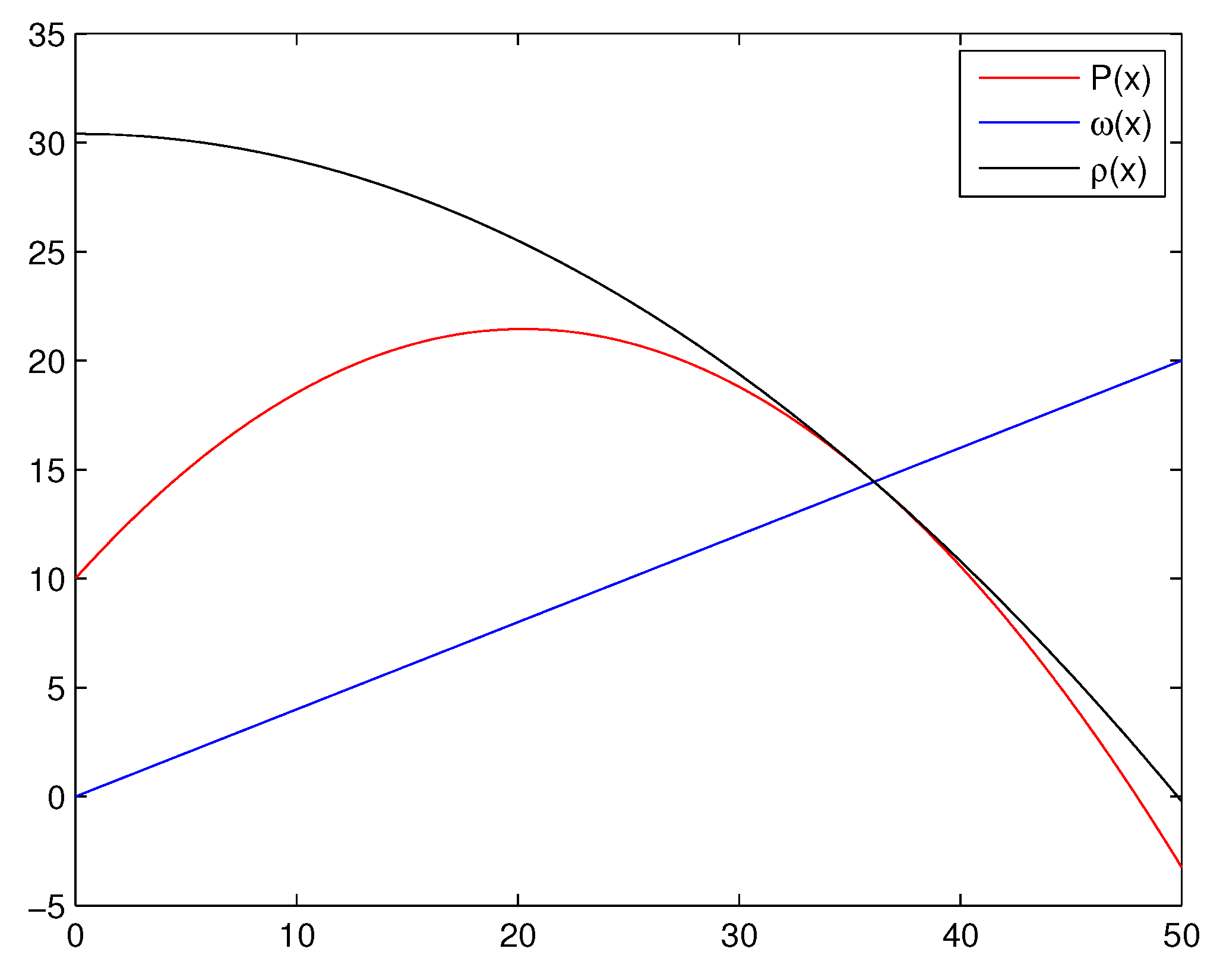
The solution to the projectile problem requires first finding $x_m$ which satisfies $\rho \left(x\right)=\omega \left(x\right)$ and solving for ${\theta }_m$ in Equation (40) because we want to find the point at which the enveloping parabola ρ intersects the impact function ω, and then find θ that corresponds to this point on the enveloping parabola. We choose a linear impact function $\omega \left(x\right)=0.4x$ with $h=10$ and $v=20$. We let $g=9.8$. Then we apply our IFs starting from $x_0=30$ to solve the non-linear equation

$$\begin{array}{cc}\hfill f\left(x\right)& =\rho \left(x\right)-\omega \left(x\right)=h+\frac{v^2}{2g}-\frac{g{x}^2}{2v^2}-0.4x\hfill \end{array}$$

whose root is given by $x_m=36.102990117.....$ and

$${\theta }_m=arctan\left(\frac{v^2}{g{x}_m}\right)={48.5}^{\circ }.$$

Figure 1 shows the intersection of the path function, the enveloping parabola and the linear impact function for this application. The approximate solutions are calculated correct to 500 significant figures. The stopping criterion $|x_N-x_{N-1}|<ϵ$, where $ϵ={10}^{-50}$ is used.

Table 6. Results of projectile problem.

IF	N	Error	$\mathit{cpu}\mathit{Time}\left(\mathit{s}\right)$	$\mathit{\rho }$
2ndNR	7	4.3980 $\times {10}^{-76}$	1.074036	1.99
4thYM	4	4.3980 $\times {10}^{-76}$	0.902015	3.99
8thKT	3	1.5610 $\times {10}^{-66}$	0.658235	8.03
8thLW	3	7.8416 $\times {10}^{-66}$	0.672524	8.03
8thPNPD	3	4.2702 $\times {10}^{-57}$	0.672042	8.05
8thSA1	3	1.2092 $\times {10}^{-61}$	0.654623	8.06
8thCTV	3	3.5871 $\times {10}^{-73}$	0.689627	8.02
8thYM	3	4.3980 $\times {10}^{-76}$	0.618145	8.02
16thYM	3	0	0.512152	16.01

shows that proposed method 16^thYM is converging better than other compared methods. Also, we observe that the computational order of convergence agrees with the theoretical order of convergence.

5.2. Planck’s Radiation Law Problem

We consider the following Planck’s radiation law problem found in [24]:

$$\phi \left(\lambda \right)=\frac{8\pi ch{\lambda }^{-5}}{e^{ch/\lambda kT}-1},$$

(44)

which calculates the energy density within an isothermal blackbody. Here, λ is the wavelength of the radiation, T is the absolute temperature of the blackbody, k is Boltzmann’s constant, h is the Planck’s constant and c is the speed of light. Suppose, we would like to determine wavelength λ which corresponds to maximum energy density $\phi \left(\lambda \right)$. From (44), we get

$${\phi }^{\prime }\left(\lambda \right)=\left(\frac{8\pi ch{\lambda }^{-6}}{e^{ch/\lambda kT}-1}\right)\left(\frac{\left(ch/\lambda kT\right)e^{ch/\lambda kT}}{e^{ch/\lambda kT}-1}-5\right)=A·B.$$

It can be checked that a maxima for φ occurs when $B=0$, that is, when

$$\left(\frac{\left(ch/\lambda kT\right)e^{ch/\lambda kT}}{e^{ch/\lambda kT}-1}\right)=5.$$

Here putting $x=ch/\lambda kT$, the above equation becomes

$$1-\frac{x}{5}=e^{-x}.$$

(45)

Define

$$f\left(x\right)=e^{-x}-1+\frac{x}{5}.$$

(46)

The aim is to find a root of the equation $f\left(x\right)=0$. Obviously, one of the root $x=0$ is not taken for discussion. As argued in [24], the left-hand side of (45) is zero for $x=5$ and $e^{-5}\approx 6.74\times {10}^{-3}$. Hence, it is expected that another root of the equation $f\left(x\right)=0$ might occur near $x=5$. The approximate root of the Equation (46) is given by $x^{\ast }\approx 4.96511423174427630369$ with $x_0=3$. Consequently, the wavelength of radiation (λ) corresponding to which the energy density is maximum is approximated as

$$\lambda \approx \frac{ch}{\left(kT\right)4.96511423174427630369}.$$

Table 7. Results of Planck’s radiation law problem.

IF	N	Error	$\mathit{cpu}\mathit{Time}\left(\mathit{s}\right)$	$\mathit{\rho }$
2ndNR	7	1.8205 $\times {10}^{-70}$	0.991020	2.00
4thYM	5	1.4688 $\times {10}^{-181}$	0.842220	4.00
8thKT	4	4.0810 $\times {10}^{-288}$	0.808787	7.99
8thLW	4	3.1188 $\times {10}^{-268}$	0.801304	7.99
8thPNPD	4	8.0615 $\times {10}^{-260}$	0.800895	7.99
8thSA1	4	1.9335 $\times {10}^{-298}$	0.791706	8.00
8thCTV	4	5.8673 $\times {10}^{-282}$	0.831006	8.00
8thYM	4	2.5197 $\times {10}^{-322}$	0.855137	8.00
16thYM	3	8.3176 $\times {10}^{-153}$	0.828053	16.52

shows that proposed method 16^thYM is converging better than other compared methods. Also, we observe that the computational order of convergence agrees with the theoretical order of convergence.

Hereafter, we will study the optimal fourth and eighth order methods along with Newton’s method.

6. Corresponding Conjugacy Maps for Quadratic Polynomials

In this section, we discuss the rational map $R_p$ arising from $2^{nd}NR$, proposed methods $4^{th}YM$ and $8^{th}YM$ applied to a generic polynomial with simple roots.

Theorem 3.

($2^{nd}NR$) [18] For a rational map $R_p\left(z\right)$ arising from Newton’s method (4) applied to $p\left(z\right)=(z-a)(z-b)$, $a\ne b$, $R_p\left(z\right)$ is conjugate via the a Möbius transformation given by $M\left(z\right)=(z-a)/(z-b)$ to

$$S\left(z\right)=z^2.$$

Theorem 4.

($4^{th}YM$) For a rational map $R_p\left(z\right)$ arising from Proposed Method (7) applied to $p\left(z\right)=(z-a)(z-b)$, $a\ne b$, $R_p\left(z\right)$ is conjugate via the a Möbius transformation given by $M\left(z\right)=(z-a)/(z-b)$ to

$$S\left(z\right)=z^4.$$

Proof. 

Let $p\left(z\right)=(z-a)(z-b)$, $a\ne b$, and let M be Möbius transformation given by $M\left(z\right)=(z-a)/(z-b)$ with its inverse $M^{-1}\left(z\right)=\frac{(zb-a)}{(z-1)}$, which may be considered as map from $\mathbb{C}\cup \{\infty \}$. We then have

$$S\left(z\right)=M\circ R_p\circ M^{-1}\left(z\right)=M\left(R_p\left(\frac{zb-a}{z-1}\right)\right)=z^4.$$

□

Theorem 5.

($8^{th}YM$) For a rational map $R_p\left(z\right)$ arising from Proposed Method (12) applied to $p\left(z\right)=(z-a)(z-b)$, $a\ne b$, $R_p\left(z\right)$ is conjugate via the a Möbius transformation given by $M\left(z\right)=(z-a)/(z-b)$ to

$$S\left(z\right)=z^8.$$

Proof. 

Let $p\left(z\right)=(z-a)(z-b)$, $a\ne b$, and let M be Möbius transformation given by $M\left(z\right)=(z-a)/(z-b)$ with its inverse $M^{-1}\left(z\right)=\frac{(zb-a)}{(z-1)}$, which may be considered as map from $\mathbb{C}\cup \{\infty \}$. We then have

$$S\left(z\right)=M\circ R_p\circ M^{-1}\left(z\right)=M\left(R_p\left(\frac{zb-a}{z-1}\right)\right)=z^8.$$

□

Remark 1.

The methods (29)–(35) are given without proof, which can be worked out with the help of Mathematica.

Remark 2.

All the maps obtained above are of the form $S\left(z\right)=z^{p}R\left(z\right)$, where $R\left(z\right)$ is either unity or a rational function and p is the order of the method.

7. Basins of Attraction

The study of dynamical behavior of the rational function associated to an iterative method gives important information about convergence and stability of the method. The basic definitions and dynamical concepts of rational function which can found in [4,25].

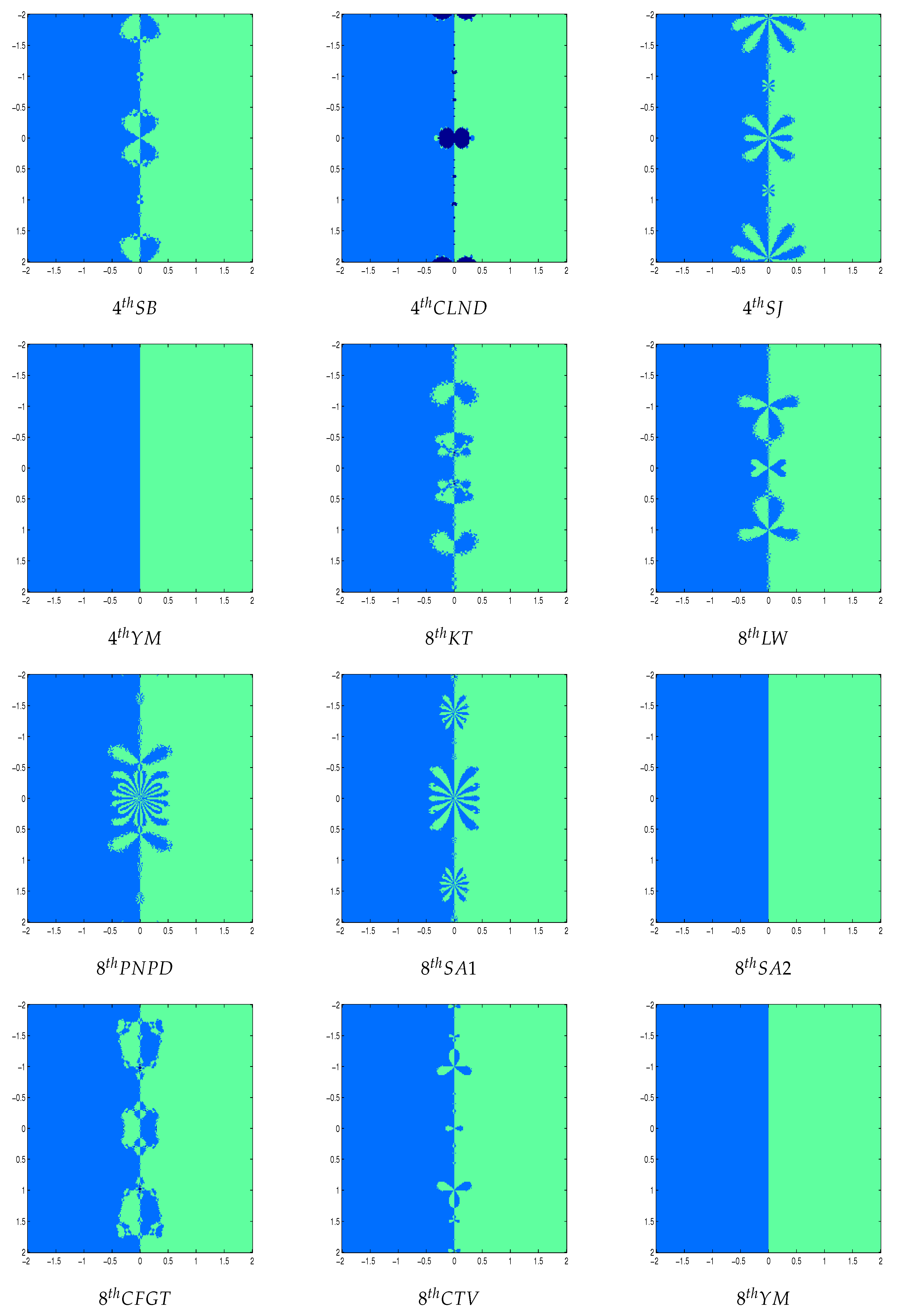
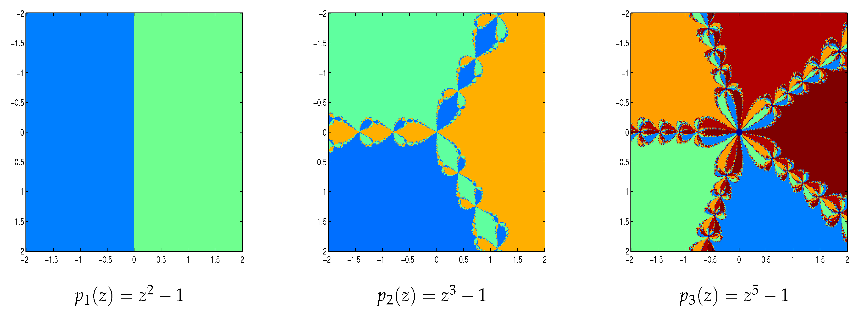
We take a square $\mathbb{R}\times \mathbb{R}=[-2,2]\times [-2,2]$ of $256\times 256$ points and we apply our iterative methods starting in every $z^{\left(0\right)}$ in the square. If the sequence generated by the iterative method attempts a zero $z_j^{\ast }$ of the polynomial with a tolerance $|f\left(z^{\left(k\right)}\right)|<\times {10}^{-4}$ and a maximum of 100 iterations, we decide that $z^{\left(0\right)}$ is in the basin of attraction of this zero. If the iterative method starting in $z^{\left(0\right)}$ reaches a zero in N iterations ($N\le 100$), then we mark this point $z^{\left(0\right)}$ with colors if $|z^{\left(N\right)}-z_j^{\ast }|<\times {10}^{-4}$. If $N>50$, we conclude that the starting point has diverged and we assign a dark blue color. Let $N_D$ be a number of diverging points and we count the number of starting points which converge in 1, 2, 3, 4, 5 or above 5 iterations. In the following, we describe the basins of attraction for Newton’s method and some higher order Newton type methods for finding complex roots of polynomials $p_1\left(z\right)=z^2-1$, $p_2\left(z\right)=z^3-1$ and $p_3\left(z\right)=z^5-1$.

Figure 2 and Figure 3 shows the polynomiographs of the methods for the polynomial $p_1\left(z\right)$. We can see that the methods 2^ndNR, 4^thYM, 8^thSA2 and 8^thYM performed very nicely. The methods 4^thSB, 4^thSJ, 8^thKT, 8^thLW, 8^thPNPD, 8^thSA1, 8^thCFGT and 8^thCTV are shows some chaotic behavior near the boundary points. The method 4^thCLND have sensitive to the choice of initial guess in this case.

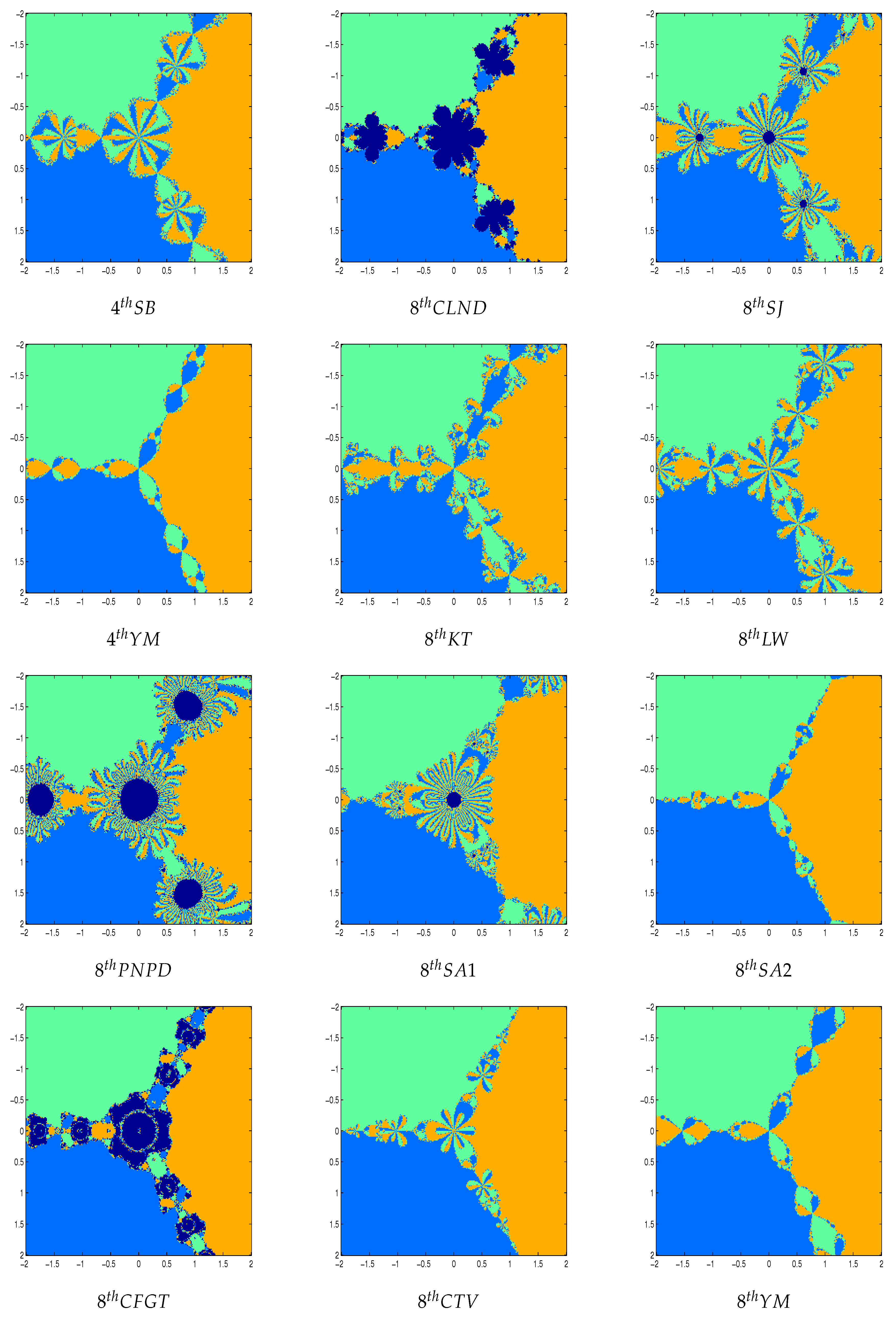
Figure 2 and Figure 4 shows the polynomiographs of the methods for the polynomial $p_2\left(z\right)$. We can see that the methods 2^ndNR, 4^thYM, 8^thSA2 and 8^thYM performed very nicely. The methods 4^thSB, 8^thKT, 8^thLW and 8^thCTV are shows some chaotic behavior near the boundary points. The methods 4^thCLND, 4^thSJ, 8^thPNPD, 8^thSA1, and 8^thCFGT have sensitive to the choice of initial guess in this case.

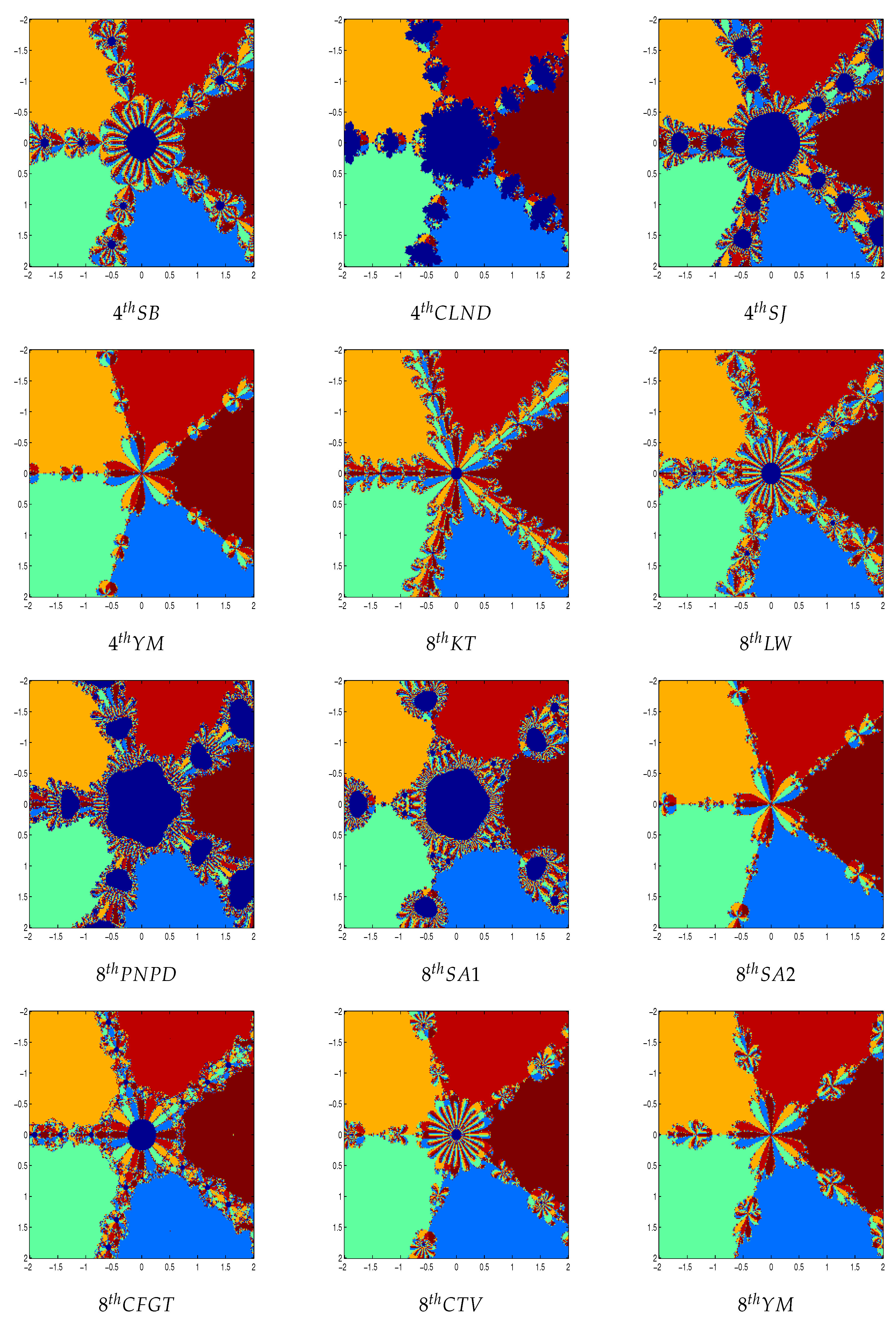
Figure 2 and Figure 5 shows the polynomiographs of the methods for the polynomial $p_3\left(z\right)$. We can see that the methods 4^thYM, 8^thSA2 and 8^thYM are shows some chaotic behavior near the boundary points. The methods 2^ndNR, 4^thSB, 4^thCLND, 4^thSJ, 8^thKT, 8^thLW, 8^thPNPD, 8^thSA1, 8^thCFGT and 8^thCTV have sensitive to the choice of initial guess in this case. In

Table 8. Results of the polynomials $p_1\left(z\right)=z^2-1$.

IF	$\mathit{N}=1$	$\mathit{N}=2$	$\mathit{N}=3$	$\mathit{N}=4$	$\mathit{N}=5$	$\mathit{N}>5$	${\mathit{N}}_{\mathit{D}}$
2ndNR	4	516	7828	23,272	20,548	13,368	0
4thSB	340	22,784	29,056	6836	2928	3592	0
4thCLND	372	24,600	29,140	6512	2224	2688	1076
4thSJ	300	19,816	28,008	5844	2968	8600	0
4thYM	520	31,100	27,520	4828	1208	360	0
8thKT	4684	44,528	9840	3820	1408	1256	24
8thLW	4452	43,236	11,408	3520	1540	1380	0
8thPNPD	2732	39,768	13,112	3480	1568	4876	16
8thSA1	4328	45,824	8136	2564	1484	3200	0
8thSA2	15,680	45,784	3696	376	0	0	0
8thCFGT	9616	43,716	7744	2916	980	564	64
8thCTV	7124	48,232	7464	1892	632	192	0
8thYM	8348	50,792	5572	824	0	0	0

,

Table 9. Results of the polynomials $p_2\left(z\right)=z^3-1$.

IF	$\mathit{N}=1$	$\mathit{N}=2$	$\mathit{N}=3$	$\mathit{N}=4$	$\mathit{N}=5$	$\mathit{N}>5$	${\mathit{N}}_{\mathit{D}}$
2ndNR	0	224	2908	11,302	19,170	31,932	0
4thSB	160	9816	27,438	9346	5452	13,324	6
4thCLND	170	11,242	28,610	9984	4202	11,328	7176
4thSJ	138	7760	25,092	8260	5058	19,228	1576
4thYM	270	18,064	30,374	9862	3688	3278	0
8thKT	2066	34,248	11,752	6130	4478	6862	0
8thLW	2092	33,968	12,180	4830	3030	9436	0
8thPNPD	1106	25,712	11,258	3854	1906	21,700	10,452
8thSA1	1608	36,488	12,486	3718	1780	9456	872
8thSA2	6432	46,850	9120	2230	640	264	0
8thCFGT	3688	40,740	13,696	4278	1390	1744	7395
8thCTV	3530	43,554	11,724	3220	1412	2096	0
8thYM	3816	43,596	12,464	3636	1302	722	0

and

Table 10. Results of the polynomials $p_3\left(z\right)=z^5-1$.

IF	$\mathit{N}=1$	$\mathit{N}=2$	$\mathit{N}=3$	$\mathit{N}=4$	$\mathit{N}=5$	$\mathit{N}>5$	${\mathit{N}}_{\mathit{D}}$
2ndNR	2	100	1222	4106	7918	52,188	638
4thSB	76	3850	15,458	18,026	5532	22,594	5324
4thCLND	86	4476	18,150	17,774	5434	19,616	12,208
4thSJ	62	3094	11,716	16,840	5682	28,142	19,900
4thYM	142	7956	27,428	15,850	5726	8434	0
8thKT	950	17,884	20,892	5675	4024	16,111	217
8thLW	1032	18,764	20,622	5056	3446	16,616	1684
8thPNPD	496	12,770	21,472	6576	2434	21,788	14,236
8thSA1	692	26,212	15,024	4060	1834	17,714	8814
8thSA2	2662	41,400	12,914	4364	1892	2304	0
8thCFGT	2008	21,194	23,734	6180	3958	8462	1953
8thCTV	1802	36,630	13,222	4112	2096	7674	350
8thYM	1736	27,808	21,136	5804	2704	6348	0

, we classify the number of converging and diverging grid points for each iterative method.

We note that a point $z_0$ belongs to the Julia set if and only if the dynamics in a neighborhood of $z_0$ displays sensitive dependence on the initial conditions, so that nearby initial conditions lead to wildly different behavior after a number of iterations. For this reason, some of the methods are getting divergent points. The common boundaries of these basins of attraction constitute the Julia set of the iteration function. It is clear that one has to use quantitative measures to distinguish between the methods, since we have a different conclusion when just viewing the basins of attraction.

In order to summarize the results, we have compared mean number of iteration and total number of functional evaluations (TNFE) for each polynomials and each methods in

Table 11. Mean number of iteration ($N_{\mu }$) and TNFE for each polynomials and each methods.

IF	${\mathit{N}}_{\mathit{\mu }}\mathit{for}{\mathit{p}}_1\left(\mathit{z}\right)$	${\mathit{N}}_{\mathit{\mu }}\mathit{for}{\mathit{p}}_2\left(\mathit{z}\right)$	${\mathit{N}}_{\mathit{\mu }}\mathit{for}{\mathit{p}}_3\left(\mathit{z}\right)$	Average	TNFE
2ndNR	4.7767	6.4317	9.8531	7.0205	14.0410
4thSB	3.0701	4.5733	9.2701	5.6378	16.9135
4thCLND	3.6644	8.6354	12.8612	8.3870	25.1610
4thSJ	3.7002	7.0909	14.5650	8.4520	25.3561
4thYM	2.6366	3.1733	4.0183	3.2760	9.8282
8thKT	2.3647	3.1270	4.4501	3.3139	13.2557
8thLW	2.3879	3.5209	6.3296	4.0794	16.3178
8thPNPD	2.9959	10.5024	12.3360	8.6114	34.4457
8thSA1	2.5097	4.5787	9.7899	5.6262	22.5044
8thSA2	1.8286	2.1559	2.5732	2.1859	8.7436
8thCFGT	2.1683	2.8029	3.4959	2.8223	11.2894
8thCTV	2.1047	2.4708	3.9573	2.8442	11.3770
8thYM	1.9828	2.3532	3.3617	2.5659	10.2636

. The best method based on the comparison in Table 11 is 8^thSA2. The method with the fewest number of functional evaluations per point is 8^thSA2 followed closely by 4^thYM. The fastest method is 8^thSA2 followed closely by 8^thYM. The method with highest number of functional evaluation and slowest method is 8^thPNPD.

8. Concluding Remarks and Future Work

In this work, we have developed optimal fourth, eighth and sixteenth order iterative methods for solving nonlinear equations using the divided difference approximation. The methods require the computations of three functions evaluations reaching order of convergence is four, four functions evaluations reaching order of convergence is eight and five functions evaluations reaching order of convergence is sixteen. In the sense of convergence analysis and numerical examples, the Kung-Traub’s conjecture is satisfied. We have tested some examples using the proposed schemes and some known schemes, which illustrate the superiority of the proposed method 16^thYM. Also, proposed methods and some existing methods have been applied on the Projectile motion problem and Planck’s radiation law problem. The results obtained are interesting and encouraging for the new method 16^thYM. The numerical experiments suggests that the new methods would be valuable alternative for solving nonlinear equations. Finally, we have also compared the basins of attraction of various fourth and eighth order methods in the complex plane.

Future work includes:

• Now we are investigating the proposed scheme to develop optimal methods of arbitrarily high order with Newton’s method, as in [26].
• Also, we are investigating to develop derivative free methods to study dynamical behavior and local convergence, as in [27,28].