Article

Application of the Laplace Homotopy Perturbation Method to the Black–Scholes Model Based on a European Put Option with Two Assets

by
Din Prathumwan
1 and
Kamonchat Trachoo
2,*
1
Department of Mathematics, Faculty of Science, Khon Kaen University, Khon Kaen 40002, Thailand
2
Department of Mathematics, Faculty of Science, Mahasarakham University, Mahasarakham 44150, Thailand
*
Author to whom correspondence should be addressed.
Mathematics 2019, 7(4), 310; https://doi.org/10.3390/math7040310
Submission received: 14 February 2019 / Revised: 13 March 2019 / Accepted: 22 March 2019 / Published: 27 March 2019

Abstract

:
In this paper, the Laplace homotopy perturbation method (LHPM) is applied to obtain the approximate solution of Black–Scholes partial differential equations for a European put option with two assets. Different from all other approximation methods, LHPM provides a simple way to get the explicit solution which is represented in the form of a Mellin–Ross function. The numerical examples represent that the solution from the proposed method is easy and effective.

1. Introduction

Over the last half century, financial behavior has become an important thing for humans. The price crashes, momentum, and bubbles are investigated for understanding the dynamics of the financial system. Recently, mathematical models are used to describe and predict the financial behavior of the market in the future [1,2,3,4,5,6,7,8,9,10,11,12]. The stock has played a major role in the financial market. The options are the essential key for the derivative which is generally used in the market. A derivative value can be obtained from many sorts of assets—for instance, interest rate, shares, currency, etc. [13,14].
In the financial market, there are many styles of options such as American, European, Asian, Canary, etc. An option is a financial contract between buyers and sellers. The option price is a premium which is obtained from the writer of the option selling options to the buyer. In general, the options can be divided into two types. These are call options that are paid for conferring the right to buy and put options that are paid for conferring the right to sell.
In this paper, we focus only on a put option for European options that may be exercised only on the expiration date of the contract due to a lack of research proposing the analytical solution of this model with two assets. The dominant benefit of the European option allows holders to buy products from sellers with an agreement involving the price and date before exercising. This process provides a benefit to the seller and buyer because an agreement can be considered before making a decision. Moreover, the criteria of this process can be applied to another process such as the purchasing of products.
To investigate the option pricing in the market, the Black–Scholes model is widely used to forecast the behavior of a European option on a stock. The Black–Scholes model was proposed by Black, Scholes, and Merton [15] in 1973. It is set up by a geometric Brownian motion and governed by a partial differential equation with respect to time and stock price. The Black–Scholes model was studied and modified for predicting the option price in the actual market [16,17,18,19]. The main key components of the Black–Scholes model are the risk-free rate, the underlying stock price, strike price, volatility, and expiration date. Recently, the option price in a market depends on other markets, which results in the multidimensional Black–Scholes model becoming more productive than the one-dimensional model. A number of methods are used to find the solution of the multi-dimensional Black–Scholes model—for example, the finite different method [13,14,20,21,22], the finite element method [23], the Mellin transform method [24], and the adaptive wavelet precise integration method [25]. Moreover, the radial basis function (RBF) based methods that are commonly used to solve the Black–Scholes equations problems; as references papers below give RBF theory [26] and applications [27,28].
The Homotopy Perturbation method (HPM), proposed by He [29], has been successfully applied to find analytical solutions for many problems in engineering, physics, biology, finance, and science [29,30,31,32,33,34,35,36]. The solutions to this method are represented as an infinite series. In particular, the solution from HPM converges rapidly to the exact solution. HPM has become a powerful tool to solve mathematical problems [30,37]. Nevertheless, HPM cannot solve some complicated problems. The Laplace homotopy perturbation method (LHPM) is introduced [38,39,40]. LHPM is a method combined with HPM and Laplace transform. For example, the explicit solutions of the Black–Scholes equation for call options are carried out by LHPM [41,42]. In this work, we study the Black–Scholes equation with the basket option based on a European put option with two assets. The Laplace transformation homotopy perturbation method is used to find the explicit approximate solution of the problem.
The remainder of this paper is organized as follows. In Section 2, we present the mathematical model that is the Black–Scholes equation with a basket option based on a European put option with two assets. Then, the concept of Laplace transform homotopy perturbation method is shown in Section 3. The explicit solution of the Black–Scholes equation for a European put option with two assets, solved by using LHPM, is presented in Section 4. The numerical simulations are obtained in Section 5. Finally, we present conclusions in Section 6.

2. The Mathematical Model

We investigated the standard two-dimensional Black–Scholes partial differential equation for European put options including efficient markets, no dividends and perfect liquidity for all of the option’s life. The two-dimensional European put option depends on the prices of two underlying assets A 1 and A 2 . The Black–Scholes model is based on
p 
the value of put option depending on the stock prices { A 1 , A 2 } at time t,
ρ 
the correlation between the two underlying stock prices A 1 and A 2 ,
wi 
the portions of underlying stock A i for i = 1 , 2 ,
Ki 
the strike price of the ith underlying stock for i = 1 , 2 ,
r 
the risk-free interest rate,
σi 
the volatility of the ith underlying stock for i = 1 , 2 ,
T 
the expiration date.
With the assumptions of the Black–Scholes model [15], the two-asset Black–Scholes option price p ( t , A 1 , A 2 ) is in the form of the partial differential equation
p τ + 1 2 σ 1 2 A 1 2 2 p A 1 2 + 1 2 σ 2 2 A 2 2 2 p A 2 2 + ρ σ 1 σ 2 A 1 A 2 2 p A 1 A 2 + r A 1 p A 1 + r A 2 p A 2 r c = 0 ,
for A 1 , A 2 [ 0 , ) , τ [ 0 , T ] , with the terminal condition:
p ( A 1 , A 2 , T ) = max ( K ( w 1 A 1 + w 2 A 2 ) , 0 ) ,
in which K = max { K 1 , K 2 } , and boundary condition
p ( 0 , A 2 , τ ) = max ( K e r ( T τ ) w 2 A 2 , 0 ) , p ( A 1 , 0 , τ ) = max ( K e r ( T τ ) w 1 A 1 , 0 ) , p ( A 1 , A 2 , τ ) = max ( K e r ( T τ ) ( w 1 A 1 + w 2 A 2 ) , 0 ) as A 1 or A 2 .
To be able to change the problem to the initial boundary value problem, we introduce a forward time t = T τ . Thus, Equation (1) can be written as
p t 1 2 σ 1 2 A 1 2 2 p A 1 2 1 2 σ 2 2 A 2 2 2 p A 2 2 ρ σ 1 σ 2 A 1 A 2 2 c A 1 A 2 r A 1 p A 1 r A 2 p A 2 + r p = 0 .
Without loss of generality, we can consider A 1 as x, and A 2 as y. Hence, this above equation becomes
p t = 1 2 σ 1 2 x 2 2 p x 2 + 1 2 σ 2 2 y 2 2 p y 2 + ρ σ 1 σ 2 x y 2 p x y + r x p x + r y p y r p .
The terminal condition becomes the initial condition as follows:
p ( x , y , 0 ) = max ( K ( w 1 A 1 + w 2 A 2 ) , 0 ) .

3. The Basic Ideas of Homotopy Perturbation Method with Laplace Transform

In general, the basic ideas of LHPM for the time-dependent differential equation are given as follows:
D ( u ( x , y , t ) ) f ( x , y , t ) = 0 ,
where D denotes a differential operator, u ( x , y , t ) denotes an unknown function and f ( x , y , t ) denotes a known analytic function. D can be determined as
D ( u ( x , y , t ) ) = t u ( x , y , t ) + N ( u ( x , y , t ) ) for ( x , y , t ) R × R × [ 0 , T ] ,
where N is the remaining part of D .
The general equation on the domain Ω = R × R × [ 0 , T ] can be written as the following equation:
t u ( x , y , t ) + N ( u ( x , y , t ) ) = f ( x , y , t ) , ( x , y , t ) Ω ,
with the initial condition
u ( x , y , 0 ) = h ( x , y ) for any ( x , y ) R × R ,
and the boundary condition:
B u , u x , u y , u t = 0 ,
where B denotes the boundary operator.
Firstly, applying the Laplace transform with respect to t on both sides of Equation (6) yields
L t u ( x , y , t ) + L N ( u ( x , y , t ) ) = L f ( x , y , t ) .
By the property of the Laplace transform for differentiation, we obtain
L u ( x , y , t ) = s 1 h ( x , y ) s 1 L N ( u ( x , y , t ) ) + s 1 L f ( x , y , t ) .
Next, we take the inverse Laplace transform to the Equation (7), so that it becomes
u ( x , y , t ) = G ( x , y , t ) L 1 s 1 L N ( u ( x , y , t ) ) ,
where the function G ( x , y , t ) represents the term resulting from the source term and the determined initial conditions and boundary conditions.
Applying the homotopy perturbation method (HPM) [31,32], the function v can be constructed
v ( x , y , t ; q ) : Ω × [ 0 , 1 ] R .
We define
H ( v ( x , y , t ; q ) , q ) = ( 1 p ) [ v ( x , y , t ; q ) v 0 ˜ ( x , y , t ) ] + q [ v ( x , y , t ; q ) G ( x , y , t ) + L 1 s 1 L N ( v ( x , y , t ; q ) ) ] = 0 ,
where q [ 0 , 1 ] is a homotopy parameter and v 0 ˜ ( x , y , t ) is an initial approximation of the Equation (8).
Equation (8) is called the homotopy equation, and it can be written as the following equation:
v ( x , y , t ; q ) = v 0 ˜ ( x , y , t ) q [ v 0 ˜ ( x , y , t ) G ( x , y , t ) + L 1 s 1 L N ( v ( x , y , t ; q ) ) ] .
From Equations (8) and (9), it easy to obtain that
q = 0 H ( v ( x , y , t ; 0 ) , 0 ) = v ( x , y , t ; 0 ) v 0 ˜ ( x , y , t ) = 0 , q = 1 H ( v ( x , y , t ; 1 ) , 1 ) = v ( x , y , t ; 1 ) G ( x , y , t ) + L 1 s 1 L N ( v ( x , y , t ; 1 ) ) = 0 .
By the technique of the homotopy perturbation method, the solution v ( x , y , t ; q ) in the Equation (9) can be expressed by the form
v ( x , y , t ; q ) = i = 0 q i v i ( x , y , t ) .
By substituting Equation (10) into Equation (9) and using HPM, it can be expressed as follows:
i = 0 q i v i ( x , y , t ) = v 0 ˜ ( x , y , t ) q [ v 0 ˜ ( x , y , t ) G ( x , y , t ) + L 1 s 1 L N ( i = 0 q i v i ( x , y , t ; p ) ) ] .
By comparing the coefficients of the corresponding term of power q on both sides of the above equation, the approximate solution v i can be written as the following recurrence relations:
v 0 ( x , y , t ) = v 0 ˜ ( x , y , t ) v 1 ( x , y , t ) = G ( x , y , t ) v 0 ˜ ( x , y , t ) L 1 s 1 L N ( v 0 ˜ ( x , y , t ) ) v m ( x , y , t ) = L 1 s 1 L N ( v m 1 ( x , y , t ) ) when m 2 .
According to the solution of Equation (10), we obtain
v ( x , y , t ; q ) = v 0 ( x , y , t ) + q v 1 ( x , y , t ) + q 2 v 2 ( x , y , t ) + q 3 v 3 ( x , y , t ) + .
By letting q converge to 1, the approximate solution in this problem (5) can be expressed as follows:
u ( x , y , t ) = v ( x , y , t ; 1 ) = v 0 ( x , y , t ) + v 1 ( x , y , t ) + v 2 ( x , y , t ) + v 3 ( x , y , t ) + .
Particularly, the series (11) approaches the explicit solution when an infinite series converges.

4. An Analytical Solution of the Black–Scholes Model for European Put Options with Two Assets by Using LHPM
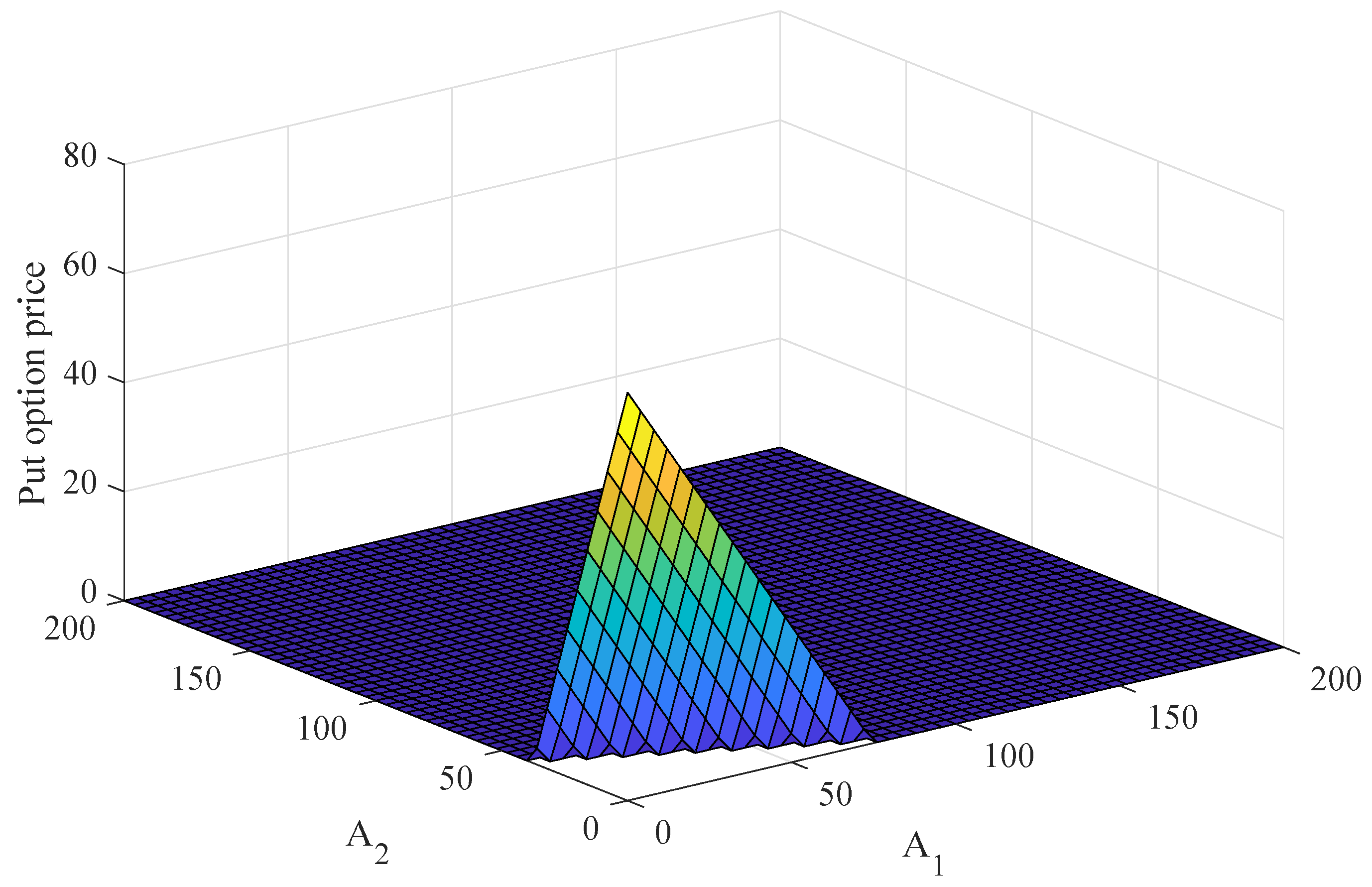
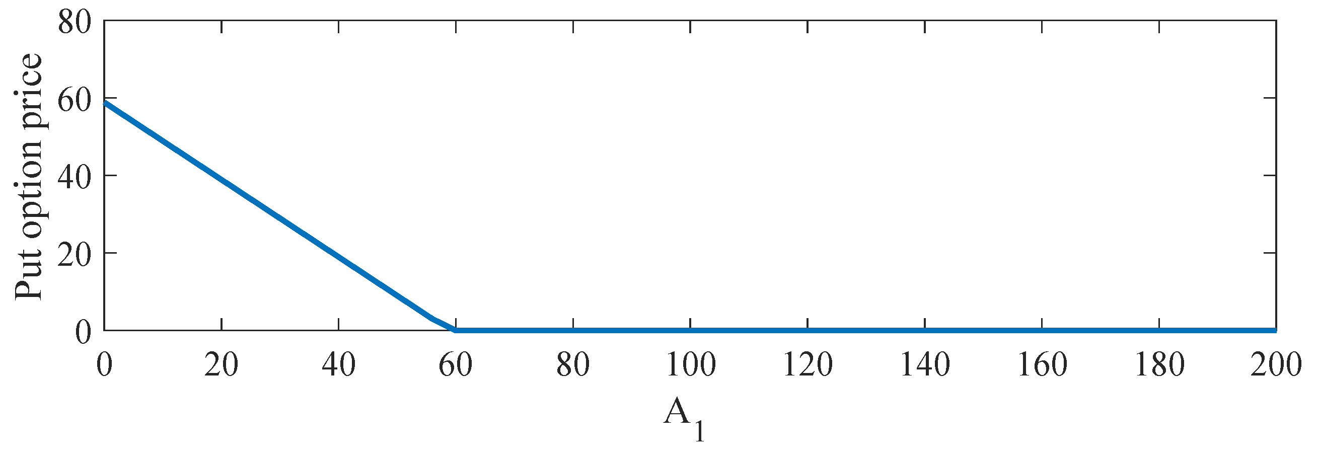
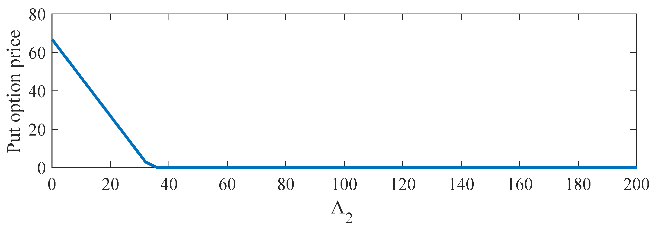
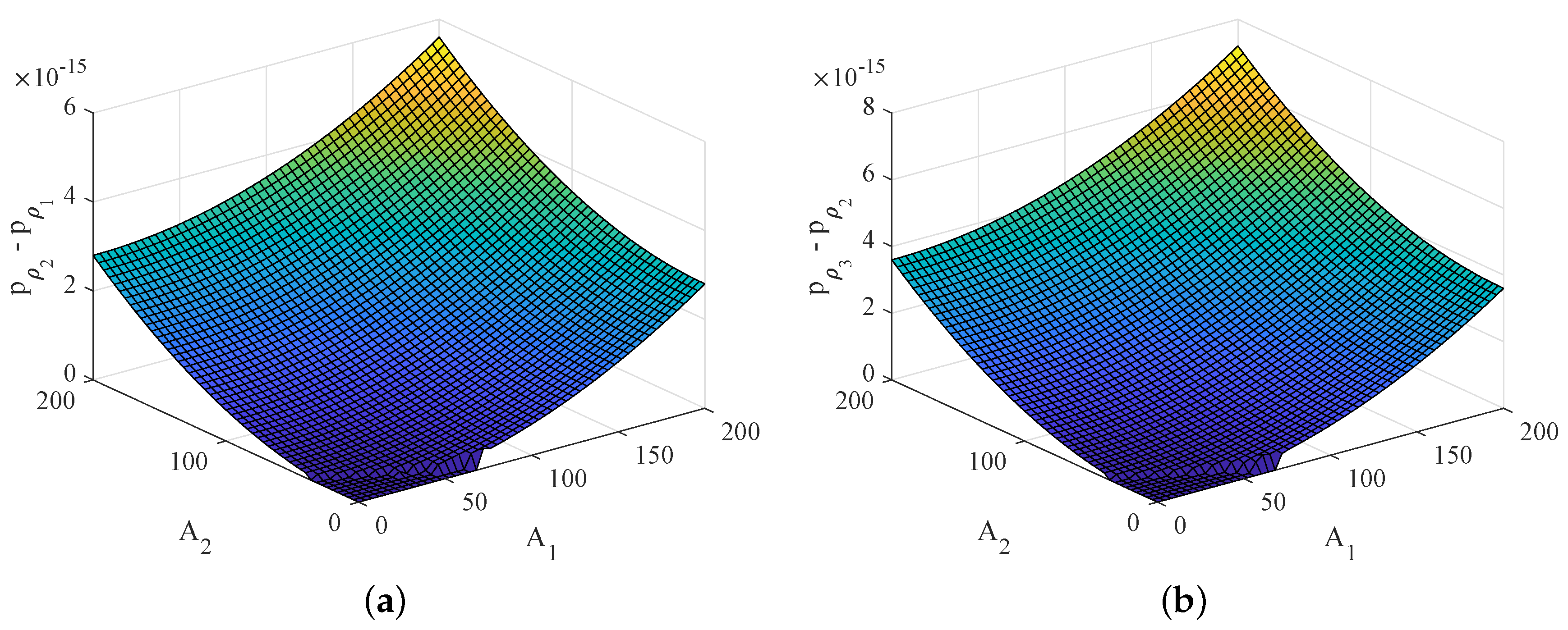
In this section, the Black–Scholes model with two assets in Equation (4) is investigated
p t = 1 2 σ 1 2 x 2 2 p x 2 + 1 2 σ 2 2 y 2 2 p y 2 + ρ σ 1 σ 2 x y 2 p x y + r x p x + r y p y r p
with the initial condition
p ( x , y , 0 ) = max ( K ( w 1 x + w 2 y ) , 0 ) .
By taking the Laplace transform with respect to t to the Equation (12), we obtain
L p t = L 1 2 σ 1 2 x 2 2 p x 2 + 1 2 σ 2 2 y 2 2 p y 2 + ρ σ 1 σ 2 x y 2 p x y + r x p x + y p y r p ,
setting
N ( p ( x , y , t ) ) = 1 2 σ 1 2 x 2 2 p x 2 + 1 2 σ 2 2 y 2 2 p y 2 + ρ σ 1 σ 2 x y 2 p x y + r x p x + y p y r p .
Equation (13) becomes
L p ( x , y , t ) = 1 s p ( x , y , 0 ) + 1 s L N ( p ( x , y , t ) ) , L p ( x , y , t ) = 1 s max ( K w 1 x w 2 y , 0 ) + 1 s L N ( p ( x , y , t ) ) .
Then, taking the inverse Laplace transform to the previous equation, we get
p ( x , y , t ) = max ( K w 1 x w 2 y , 0 ) + L 1 1 s L N ( p ( x , y , t ) ) .
Applying the Homotopy Perturbation Method, we can construct the following equation:
( 1 q ) ( p ( x , y , t ; q ) p 0 ˜ ( x , y , t ) ) + q [ p ( x , y , t ; q ) max ( K w 1 x w 2 y , 0 ) L 1 1 s L N ( p ( x , y , t ; q ) ) = 0
or we can write
p ( x , y , t ; q ) = p 0 ˜ ( x , y , t ) q p 0 ˜ ( x , y , t ) + q max ( K w 1 x w 2 y , 0 ) + q L 1 1 s L N ( p ( x , y , t ; q ) ) ,
where p 0 ˜ ( x , y , t ) is an initial approximation of Equation (14) that can be freely chosen.
For this model, we choose p 0 ˜ ( x , y , t ) in the form
p 0 ˜ ( x , y , t ) = max ( K w 1 x w 2 y , 0 ) + ρ ( x 2 + y 2 ) t .
By substituting p 0 ˜ ( x , y , t ) to Equation (14), we have
p ( x , y , t ; q ) = max ( K w 1 x w 2 y , 0 ) + ρ ( x 2 + y 2 ) t + q [ ( x 2 + y 2 ) t + L 1 1 s L N ( p ( x , y , t ; q ) ) ] .
By the HPM technique, we assume the solution of problem (15) to be written in the form
p ( x , y , t ; q ) = n = 0 q n p n ( x , y , t ) .
Substituting Equation (16) into Equation (15), we get
n = 0 q n p n ( x , y , t ) = max ( K w 1 x w 2 y , 0 ) + ρ ( x 2 + y 2 ) t + q ( x 2 + y 2 ) t + L 1 { 1 s L { 1 2 σ 1 2 x 2 n = 0 q n 2 p n x 2 + 1 2 σ 2 2 y 2 n = 0 q n 2 p n y 2 + ρ σ 1 σ 2 x y n = 0 q n 2 p n x y + r x n = 0 q n p n x + y n = 0 q n p n y r n = 0 q n p n } } .
Equating the corresponding power of p on both sides, we obtain the following:
q 0 ; p 0 ( x , y , t ) = max ( K w 1 x w 2 y , 0 ) + ρ ( x 2 + y 2 ) t , q 1 ; p 1 ( x , y , t ) = t 2 ρ 2 ( σ 1 2 + r ) x 2 + ( σ 2 2 + r ) y 2 t [ ( σ 1 2 + r ) 0 x 2 + ( σ 2 2 + r ) 0 y 2 r ( max ( w 1 , 0 ) x + max ( w 2 , 0 ) y ) + r max ( K w 1 x w 2 y , 0 ) ] , q 2 ; p 2 ( x , y , t ) = t 3 ρ 6 ( σ 1 2 + r ) 2 x 2 + ( σ 2 2 + r ) 2 y 2 t 2 2 [ ( σ 1 2 + r ) 1 x 2 + ( σ 2 2 + r ) 1 y 2 + r 2 ( max ( w 1 , 0 ) x + max ( w 2 , 0 ) y ) r 2 max ( K w 1 x w 2 y , 0 ) ] , q 3 ; p 3 ( x , y , t ) = t 4 ρ 24 ( σ 1 2 + r ) 3 x 2 + ( σ 2 2 + r ) 3 y 2 t 3 6 [ ( σ 1 2 + r ) 2 x 2 + ( σ 2 2 + r ) 2 y 2 r 3 ( max ( w 1 , 0 ) x + max ( w 2 , 0 ) y ) + r 3 max ( K w 1 x w 2 y , 0 ) ] ,
and so on.
Proceeding in the same process, we obtain
q 0 ; p 0 ( x , y , t ) = max ( K w 1 x w 2 y , 0 ) + ρ ( x 2 + y 2 ) t , q n ; p n ( x , y , t ) = t n + 1 ρ Γ ( n + 2 ) ( σ 1 2 + r ) n x 2 + ( σ 2 2 + r ) n y 2 t n Γ ( n + 1 ) [ ( σ 1 2 + r ) n 1 x 2 + ( σ 2 2 + r ) n 1 y 2 + ( 1 ) n r n ( max ( w 1 , 0 ) x + max ( w 2 , 0 ) y ) ( 1 ) n r n max ( K w 1 x w 2 y , 0 ) ] when n 1 .
Thus, the solution p ( x , y , t ; p ) of problem (15) is given by
p ( x , y , t ; q ) = n = 0 q n p n ( x , y , t ) = p 0 ( x , y , t ) + n = 1 q n { t n + 1 ρ Γ ( n + 2 ) ( σ 1 2 + r ) n x 2 + ( σ 2 2 + r ) n y 2 t n Γ ( n + 1 ) [ ( σ 1 2 + r ) n 1 x 2 + ( σ 2 2 + r ) n 1 y 2 + ( 1 ) n r n ( max ( w 1 , 0 ) x + max ( w 2 , 0 ) y ) ( 1 ) n r n max ( K w 1 x w 2 y , 0 ) ] } = p 0 ( x , y , t ) + n = 0 q n + 1 { t n + 2 ρ Γ ( n + 3 ) ( σ 1 2 + r ) n + 1 x 2 + ( σ 2 2 + r ) n + 1 y 2 t n + 1 Γ ( n + 2 ) [ ( σ 1 2 + r ) n x 2 + ( σ 2 2 + r ) n y 2 + ( 1 ) n + 1 r n + 1 ( max ( w 1 , 0 ) x + max ( w 2 , 0 ) y ) ( 1 ) n + 1 r n + 1 max ( K w 1 x w 2 y , 0 ) ] } .
By setting q converges to 1, we obtain
p ( x , y , t ) = p 0 ( x , y , t ) + n = 0 { t n + 2 ρ Γ ( n + 3 ) ( σ 1 2 + r ) n + 1 x 2 + ( σ 2 2 + r ) n + 1 y 2 t n + 1 Γ ( n + 2 ) [ ( σ 1 2 + r ) n x 2 + ( σ 2 2 + r ) n y 2 + ( 1 ) n + 1 r n + 1 ( max ( w 1 , 0 ) x + max ( w 2 , 0 ) y ) ( 1 ) n + 1 r n + 1 max ( K w 1 x w 2 y , 0 ) ] } .
Therefore, we obtain the explicit solution of problem (12) as follows:
p ( x , y , t ) = max ( K w 1 x w 2 y , 0 ) + x 2 ρ ( σ 1 2 + r ) E 2 , σ 1 2 + r ( t ) E 1 , σ 1 2 + r ( t ) + ρ t + y 2 ρ ( σ 2 2 + r ) E 2 , σ 2 2 + r ( t ) E 1 , σ 2 2 + r ( t ) + ρ t r max ( w 1 , 0 ) x + max ( w 2 , 0 ) y E 1 , r ( t ) + r max ( K w 1 x w 2 y , 0 ) E 1 , r ( t ) ,
where E a , b ( t ) = t a k = 0 ( b t ) k Γ ( a + k + 1 ) is the Mellin–Ross function [43], which a and b being constants.

5. Solution Example

In this section, the explicit solution of the problem (12) as shown in Equation (17) is computed to obtain the value of European put option with the condition as in Equation (2) and w 1 = 2 , w 2 = 1 ,
p ( A 1 , A 2 , T ) = max ( K ( 2 A 1 + A 2 ) , 0 ) ,
with strike price K = 75 . The risk-free interest rate is 5 % per year, ( r = 0.05 ) , the volatilities of the underlying assets A 1 and A 2 are σ 1 = 5 % and σ 2 = 10 % , respectively. The expiration time is T = 1 measured in years.
The solution surface plot of a European put option with the correlation, ρ = 0.8 at the maturity time is showed in Figure 1. The stock prices are considered over the range 0 A 1 200 and 0 A 2 200 which surround the strike price. The result shows that the option price linearly decreases when the stock prices, A 1 and A 2 , increase. After that, the option price reaches zero when the stock prices increase.
At a day before an expiration date, the value of put option price with the influence of stock price A 1 and fixed stock price A 2 is presented in Figure 2. The result indicated that the option price linearly dropped until the value of stock price A 1 was around 60; and the option price p reaches zero. In addition, the value of put option price with the influence of stock price A 2 and fixed stock price A 1 is also represented in Figure 3. The solution p is decreased linearly when the stock price is lower than 40 and the option price reaches zero when the stock price is greater than 40.
The different values of European put options for non-positive correlation case ρ 1 = 0.8 and ρ 2 = 0 and non-negative correlation case ρ 2 = 0 and ρ 3 = 0.8 are plotted over a range of stock prices 0 A 1 200 and 0 A 2 200 at the maturity time, as shown in Figure 4. The results show that the correlation has an effect on the European put option. Furthermore, when stock prices both increase, this leads to an increase in the difference between the value of the European put options.

6. Conclusions

The Black–Scholes model is the most famous and useful mathematical model for describing the behavior of the financial market. In this work, the Black–Scholes model for a European put option with two assets is investigated. The LHPM is applied to find the explicit solution of the Black–Scholes model in the form of the infinite series, which is a special function, called the Mellin–Ross function. The advantage of the explicit solution of the Black–Scholes model is easy to implement for simulating the option price that depends on two asset prices. Moreover, the results can be easy to apply in real world problems for the financial system.

Author Contributions

Conceptualization, D.P. and K.T.; Formal analysis, D.P. and K.T.; Methodology, D.P. and K.T.; Validation, K.T.; Visualization, K.T.; Writing—original draft, D.P.; Writing—review and editing, D.P. and K.T.

Funding

This research received no external funding.

Conflicts of Interest

The authors declare no conflict of interest.

References

  1. Cesare, L.D.; Sportelli, M. A dynamic IS-LM model with delayed taxation revenues. Chaos Solitons Fractals 2005, 25, 233–244. [Google Scholar] [CrossRef]
  2. Fanti, L.; Manfredi, P. Chaotic business cycles and fiscal policy: An IS-LM model with distributed tax collection lags. Chaos Solitons Fractals 2007, 32, 736–744. [Google Scholar] [CrossRef]
  3. He, X.Z.; Li, K.; Wei, J.; Zheng, M. Market stability switches in a continuous-time financial market with heterogeneous beliefs. Econ. Model. 2009, 26, 1432–1442. [Google Scholar] [CrossRef]
  4. Ma, J.H.; Chen, Y.S. Study for the bifurcation topological structure and the global complicated character of a kind of nonlinear finance system, I. Appl. Math. Mech. 2001, 22, 1240–1251. [Google Scholar] [CrossRef]
  5. Ma, J.H.; Chen, Y.S. Study for the bifurcation topological structure and the global complicated character of a kind of nonlinear finance system, II. Appl. Math. Mech. 2001, 22, 1375–1382. [Google Scholar] [CrossRef]
  6. He, X.Z.; Zheng, M. Dynamics of moving average rules in a continuous-time financial market model. J. Econ. Behav. Organ. 2010, 76, 615–634. [Google Scholar] [CrossRef]
  7. Chiarella, C.; He, X.Z.; Zheng, M. An analysis of the effect of noise in a heterogeneous agent financial market model. J. Econ. Dyn. Control 2011, 35, 148–162. [Google Scholar] [CrossRef]
  8. Zhou, L.; Li, Y. A generalized dynamic IS-LM model with delayed time in investment processes. Appl. Math. Comput. 2008, 196, 774–781. [Google Scholar] [CrossRef]
  9. Chatterjee, P.; Shukayev, M. A stochastic dynamic model of trade and growth: Convergence and diversification. J. Econ. Dyn. Control 2012, 36, 416–432. [Google Scholar] [CrossRef]
  10. Yang, H.; Li, L.; Wang, D. Research on the Stability of Open Financial System. Entropy 2015, 17, 1734–1754. [Google Scholar] [CrossRef]
  11. Prathumwan, D.; Sawangtong, W.; Wiwattanapataphee, B.; Giannini, L.M. A differential evolution algorithm for parameter optimization of an asset flow model. J. Algebra Appl. Math. 2019, 17, 33–56. [Google Scholar]
  12. Prathumwan, D.; Sawangtong, W.; Sawangtong, P. An Analysis on the Fractional Asset Flow Differential Equations. Mathematics 2017, 5, 33. [Google Scholar] [CrossRef]
  13. Cen, Z.; Le, A. A robust finite difference scheme for pricing american put options with singularity-separating method. Numer. Algorithms 2010, 53, 497–510. [Google Scholar] [CrossRef]
  14. Cen, Z.; Le, A. A robust and accurate finite difference method for a generalized Black–Scholes equation. J. Comput. Appl. Math. 2011, 235, 2728–2733. [Google Scholar] [CrossRef]
  15. Black, F.; Scholes, M. The pricing of options and corporate liabilities. J. Political Econ. 1973, 81, 637–654. [Google Scholar] [CrossRef]
  16. Gu¨lkac, V. The homotopy pertubation method for the Black–Scholes equation. J. Stat. Comput. Simul. 2010, 80, 1349–1354. [Google Scholar] [CrossRef]
  17. Paliathanasis, A.; Morris, R.M.; Leach, P.G.L. Lie Symmetries of (1+2) Nonautonomous Evolution Equations in Financial Mathematics. Mathematics 2016, 4, 34. [Google Scholar] [CrossRef]
  18. Rigatos, G.; Siano, P. Stabilization of the multi-asset Black–Scholes PDE using differential flatness theory. IFAC-Papers OnLine 2016, 49, 180–185. [Google Scholar] [CrossRef]
  19. Hicks, W. PT Symmetry, Non-Gaussian Path Integrals, and the Quantum Black–Scholes Equation. Entropy 2019, 21, 105. [Google Scholar] [CrossRef]
  20. Cox, J.C.; Ross, S.; Rubinstein, M. Option pricing: A simplified approach. J. Financ. Econ. 1979, 7, 229–263. [Google Scholar] [CrossRef]
  21. Lesmana, D.C.; Wang, S. An upwind finite difference method for a nonlinear Black–Scholes equation governing European option valuation under transaction costs. J. Appl. Math. Comput. 2013, 219, 8811–8828. [Google Scholar] [CrossRef]
  22. Song, L.; Wang, W. Solution of the fractional Black–Scholes option pricing model by finite difference method. Abstr. Appl. Anal. 2013, 2013, 194286. [Google Scholar] [CrossRef]
  23. Phaochoo, P.; Luadsong, A.; Aschariyaphotha, N. The meshless local Petrov–Galerkin based on moving kriging interpolation for solving fractional Black–Scholes model. J. King Saud Univ.-Sci. 2016, 28, 111–117. [Google Scholar] [CrossRef]
  24. Jodar, L.; Sevilla-Peris, P.; Cortes, J.C.; Sala, R. A new direct method for solving the Black–Scholes equation. Appl. Math. Lett. 2002, 18, 29–32. [Google Scholar] [CrossRef]
  25. Yan, H. Adaptive Wavelet Precise Integration Method for Nonlinear Black–Scholes Model Based on Variational Iteration Method. Abstr. Appl. Anal. 2013, 2013, 735919. [Google Scholar] [CrossRef]
  26. Cavoretto, R.; Schneider, T.; Zulian, P. OpenCL Based Parallel Algorithm for RBF-PUM Interpolation. J. Sci. Comput. 2018, 74, 267–289. [Google Scholar] [CrossRef]
  27. Safdari-Vaighani, A.; Heryudono, A.; Larsson, E. A Radial Basis Function Partition of Unity Collocation Method for Convection–Diffusion Equations Arising in Financial Applications. J. Sci. Comput. 2015, 64, 341–367. [Google Scholar] [CrossRef]
  28. Shcherbakov, V.; Larsson, E. Radial basis function partition of unity methods for pricing vanilla basket options. Comput. Math. Appl. 2016, 71, 185–200. [Google Scholar] [CrossRef]
  29. He, J.H. Homotopy perturbation method: A new nonlinear analytical technique. Appl. Math. Comput. 2003, 135, 73–79. [Google Scholar] [CrossRef]
  30. He, J.H. The homotopy perturbation method for nonlinear oscillations with discontinuities. Appl. Math. Comput. 2004, 151, 287–292. [Google Scholar]
  31. He, J.H. Homotopy perturbation method for bifurcation of nonlinear problems. Int. J. Nonlinear Sci. Numer. Simul. 2005, 6, 207–208. [Google Scholar] [CrossRef]
  32. He, J.H. Homotopy perturbation technique. Comput. Methods Appl. Mech. Eng. 1999, 178, 257–262. [Google Scholar] [CrossRef]
  33. Khan, Y. A novel Laplace decomposition method for non-linear stretching sheet problem in the presence of MHD and slip condition. Int. J. Numer. Methods Heat Fluid Flow 2014, 24, 73–85. [Google Scholar] [CrossRef]
  34. Khan, Y.; Abdou, M.A.; Faraz, N.; Yildirim, A.; Wu, Q. Numerical Solution of MHD Flow over a Nonlinear Porous Stretching Sheet. Iran. J. Chem. Chem. Eng. 2012, 31, 125–132. [Google Scholar]
  35. Madani, M.; Khan, Y.; Fathizadeh, M.; Yildirim, A. Application of homotopy perturbation and numerical methods to the magneto-micropolar fluid flow in the presence of radiation. Eng. Comput. 2012, 29, 277–294. [Google Scholar] [CrossRef]
  36. Shateyi, S.; Motsa, S.S.; Khan, Y. A new piecewise spectral homotopy analysis of the Michaelis-Menten enzymatic reactions model. Numer. Algorithms 2014, 66, 495–510. [Google Scholar] [CrossRef]
  37. Baholian, E.; Azizi, A.; Saeidian, J. Some notes on using the homotopy perturbation method for solving time-dependent differential equations. Math. Comput. Model. 2009, 50, 213–224. [Google Scholar] [CrossRef]
  38. Khan, Y.; Wu, Q. Homotopy perturbation transform method for nonlinear equations using He’s polynomials. Comput. Math. Appl. 2011, 61, 1963–1967. [Google Scholar] [CrossRef]
  39. Kumar, S.; Yildirim, A.; Khan, Y.; Jafari, H.; Sayevand, K.; Wei, L. Analytical Solution of Fractional Black–Scholes European Option Pricing Equation by using Laplace Transform. J. Fract. Calc. Appl. 2012, 2, 1–9. [Google Scholar]
  40. Madani, M.; Fathizadeh, M.; Khan, Y.; Yildirim, A. On the coupling of the homotopy perturbation method and Laplace transformation. Math. Comput. Model. 2011, 53, 1937–1945. [Google Scholar] [CrossRef]
  41. Sawangtong, P.; Trachoo, K.; Sawangtong, W.; Wiwattanapataphee, B. The Analytical Solution for the Black–Scholes Equation with Two Assets in the Liouville-Caputo Fractional Derivative Sense. Mathematics 2018, 6, 129. [Google Scholar] [CrossRef]
  42. Trachoo, K.; Sawangtong, W.; Sawangtong, P. Laplace Transform Homotopy Perturbation Method for the Two Dimensional Black–Scholes Model with European Call Option. Math. Comput. Appl. 2017, 22, 23. [Google Scholar] [CrossRef]
  43. Mathai, A.M.; Haubold, H.J. Special Functions for Applied Scientists; Springer: New York, NY, USA, 2008. [Google Scholar]
Figure 1. The explicit solution surface plot of the European put option price obtained from the Black–Scholes model with two stock prices, A 1 , A 2 and correlation ρ = 0 . 8 .
Mathematics 07 00310 g001
Figure 2. The solution plots of the European put option obtained from the Black–Scholes model with two stock prices for A 2 = 8 .
Mathematics 07 00310 g002
Figure 3. The solution plots of the European put option obtained from Black–Scholes model with two stock prices for A 1 = 8 .
Mathematics 07 00310 g003
Figure 4. The different values of the European put option: (a) p ρ 2 p ρ 1 and (b) p ρ 3 p ρ 2 at the maturity T with stock prices A 1 , A 2 and correlations ρ 1 = 0 . 8 , ρ 2 = 0 and ρ 3 = 0 . 8 .
Mathematics 07 00310 g004

