A General Algorithm for the Split Common Fixed Point Problem with Its Applications to Signal Processing

Abstract

In 2014, Cui and Wang constructed an algorithm for demicontractive operators and proved some weak convergence theorems of their proposed algorithm to show the existence of solutions for the split common fixed point problem without using the operator norm. By Cui and Wang’s motivation, in 2015, Boikanyo constructed also a new algorithm for demicontractive operators and obtained some strong convergence theorems for this problem without using the operator norm. In this paper, we consider a viscosity iterative algorithm in Boikanyo’s algorithm to approximate to a solution of this problem and prove some strong convergence theorems of our proposed algorithm to a solution of this problem. Finally, we apply our main results to some applications, signal processing and others and compare our algorithm with five algorithms such as Cui and Wang’s algorithm, Boikanyo’s algorithm, forward-backward splitting algorithm and the fast iterative shrinkage-thresholding algorithm (FISTA).

1. Introduction

Assume that C and Q are nonempty closed convex subsets of Hilbert spaces $H_1$ and $H_2$, respectively. Assume that $A:H_1\to H_2$ is a bounded linear operator with the adjoint $A^{\ast }$.

In 1994, the split feasibility problem was proposed by Censor and Elfving [1] as follows:

$$\mathrm{Find}\mathrm{a}\mathrm{point}{x}^{\ast }\in H_1\mathrm{such}\mathrm{that}{x}^{\ast }\in C\mathrm{and}A{x}^{\ast }\in Q.$$

(1)

It is interesting to note that, when taking $C=H_1$ and $Q=\left\{b\right\}$, the split feasibility problem reduces to the linear inverse problem:

$$\mathrm{Find}\mathrm{a}\mathrm{point}{x}^{\ast }\in H_1\mathrm{such}\mathrm{that}A{x}^{\ast }=b.$$

(2)

The most popular ways for solving the linear inverse problem is to reformulate it as a least squares problem. Similarly, the split feasibility problem was solved by equivalently reformulating it as the convex optimization problem:

$$\underset{x\in C}{min}\frac{1}{2}{\Vert Ax-P_Q\left(Ax\right)\Vert }^2,$$

(3)

where $P_Q(·)$ is the projection operator on set Q defined by

$$P_Q\left(v\right)=\underset{z\in Q}{arg\; min}\Vert z-v\Vert .$$

In 2002, based on the reformulation (3), the so-called CQ algorithm was presented by Byrne. He solved this problem by using the algorithm: For an arbitrary $x_1\in H$,

$$\begin{array}{c}\hfill x_{n+1}=A^{-1}{P}_Q\left(P_{A\left(C\right)}\left(A{x}_n\right)\right),\forall n\in \mathbb{N},\end{array}$$

(4)

which converges to a solution of the convex optimization problem. Since the algorithm (4) requires the inverse matrix of A, it is disadvantage to calculate this algorithm. We note that $x^{\ast }\in H$ solves the problem (2) is equivalent to the fixed point problem, that is, $x^{\ast }$ is a fixed point of T, where $T:=P_C(I-\rho A^{\ast }(I-P_Q)A)$ for any $\rho >0$.

In 2002, Byrne [2] constructed the following algorithm (5), which does not compute the inverse matrix of A: For any $x_0$, $\left\{x_n\right\}$ is generated by

$$\begin{array}{c}\hfill x_{n+1}=P_C(I-\rho A^{\ast }(I-P_Q)A)x_n,\forall n\in \mathbb{N},\end{array}$$

(5)

where $\rho \in (0,\frac{2}{L})$ and L is the largest eigenvalue of $A^{\ast }A$.

Recently, the split feasibility problem has been apllied to approximation theory, signal processing, image recovery, control theory, biomedical engineering, geophysics and communications by many authors. Refer to the papers [3,4,5,6,7,8,9].

Especially, the split common fixed point problem is as follows:

$$\begin{array}{c}\hfill \mathrm{Find}\mathrm{a}\mathrm{point}{x}^{\ast }\in H\mathrm{such}\mathrm{that}{x}^{\ast }\in Fix\left(U\right)\mathrm{and}A{x}^{\ast }\in Fix\left(T\right),\end{array}$$

(6)

where $U:H\to H$ and $T:K\to K$ are operators, $Fix\left(U\right)$ and $Fix\left(T\right)$ denote the fixed point sets of U and T, respectively. In 2009, this problem was proposed by Censor and Segal [10] and they constructed the following algorithm for solving the problem: For any $x_0\in H$, $\left\{x_n\right\}$ is generated by

$$\begin{array}{c}\hfill x_{n+1}=U(I-\rho A^{\ast }(I-T)A)x_n,\forall n\in \mathbb{N}.\end{array}$$

(7)

This algorithm can be extended to many cases as follows:

• Quasi-nonexpansive operators by Moudafi [11];
• Finitely many directed operators by Wang and Xu [12];
• Demicontractive operators by Moudafi [13]. In the case when U and T are directed operators, the step size $\rho$ satisfies $0<\rho <\frac{2}{{\Vert A\Vert }^2}$ and $\left\{x_n\right\}$ generated by the algorithm (7) converges weakly to a solution of the problem (6) when a solution exists.

The algorithm (7) needs to compute $\Vert A\Vert$, which is not easily computed. In 2014, Cui and Wang [14] proposed the following Algorithm 1 without using the operator norm: For an initial $x_0\in H$,

$$\begin{array}{c}\hfill \begin{array}{ccc}{x}_{n+1}\hfill & =\hfill & U_{\lambda }(x_n-{\rho }_n{A}^{\ast }(I-T)A{x}_n),\forall n\ge 0,\hfill \end{array}\end{array}$$

(8)

where

$${\rho }_n=\left\{\begin{array}{cc}\frac{(1-\tau )\Vert (I-T)A{x}_n{\Vert }^2}{2\Vert A^{\ast }(I-T)A{x}_n{\Vert }^2},\hfill & A{x}_n\ne T\left(x_n\right),\hfill \\ 0\hfill & \mathrm{otherwise},\hfill \end{array}\right.$$

where U and T are demicontractive operators with constants $0\le \kappa <1$ and $0\le \tau <1$ such that $I-U$ and $I-T$ are demiclosed at zero, respectively, denote $U_{\lambda }:=(1-\lambda )I+\lambda U$ for any $\lambda \in (0,1-\kappa )$ and A is a bounded linear operator, and they proved that the algorithm (8) converges weakly to a solution of the problem (6) when a solution exists.

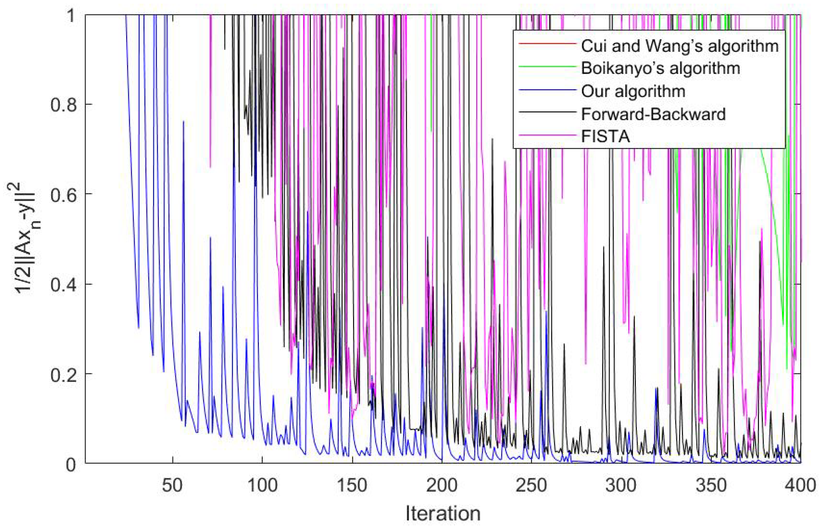
Algorithm 1: Cui and Wang’s algorithm

Input: Set $\lambda \in (0,1-\kappa )$, where $0\le \kappa <1$. Choose $x_0\in H$. 1 for $n=1,2,\cdots$ do 2   Update $x_{n+1}$ via (8), 3 end for

In 2015, Boikanyo [15] extended Cui and Wang’s results and proposed the following Algorithm 2 for demicontrative operators U and T with $U_{\lambda }:=(1-\lambda )I+\lambda U$ for any $\lambda \in (0,1-\kappa )$, which converges strongly to a solution of the problem (6) when a solution exists: For any $u\in H$,

$$\begin{array}{c}\hfill \begin{array}{ccc}{x}_{n+1}\hfill & =\hfill & {\alpha }_{n}u+(1-{\alpha }_n)U_{\lambda }(x_n-{\rho }_n{A}^{\ast }(I-T)A{x}_n),\forall n\ge 0,\hfill \end{array}\end{array}$$

(9)

where

$${\rho }_n=\left\{\begin{array}{cc}\frac{(1-\tau )\Vert (I-T)A{x}_n{\Vert }^2}{2\Vert A^{\ast }(I-T)A{x}_n{\Vert }^2},\hfill & A{x}_n\ne T\left(x_n\right),\hfill \\ 0\hfill & \mathrm{otherwise},\hfill \end{array}\right.$$

and $\left\{{\alpha }_n\right\}$ is a sequence in $[0,1)$ such that

$$\underset{n\to \infty }{lim}{\alpha }_n=0,\sum _{n=0}^{\infty }{\alpha }_n=\infty .$$

Algorithm 2: Boikanyo’s algorithm

Input: Set $\lambda \in (0,1-\kappa )$ where $0\le \kappa <1$, and ${\alpha }_n\in [0,1)$ such that $\underset{n\to \infty }{lim}{\alpha }_n=0$ and ${\displaystyle \sum _{n=0}^{\infty }}{\alpha }_n=\infty$. Choose $u,x_0\in H$. 1 for $n=1,2,\cdots$ do 2   Update $x_{n+1}$ via (9). 3 end for

In 2016, Huimin et al. [16] proposed the following Algorithm 3 for demicontrative operators U, T with $U_{\lambda }:=(1-\lambda )I+\lambda U$ for any $\lambda \in (0,1-\kappa )$, where $\lambda \in (0,1-\kappa )$, and f is a contraction operator on $Fix\left(U\right)$ which converges strongly to a solution of the problem (6) when a solution exists:

$$\begin{array}{c}\hfill \begin{array}{ccc}{x}_{n+1}\hfill & =\hfill & {\alpha }_{n}f\left(x_n\right)+(1-{\alpha }_n)U_{\lambda }(x_n-{\rho }_n{A}^{\ast }(I-T)A{x}_n),\forall n\ge 0,\hfill \end{array}\end{array}$$

(10)

where

$${\rho }_n=\left\{\begin{array}{cc}\frac{(1-\tau )\Vert (I-T)A{x}_n{\Vert }^2}{2\Vert A^{\ast }(I-T)A{x}_n{\Vert }^2},\hfill & A{x}_n\ne T\left(x_n\right),\hfill \\ 0\hfill & \mathrm{otherwise},\hfill \end{array}\right.$$

and $\left\{{\alpha }_n\right\}$ is a sequence in $[0,1)$ such that

$$\underset{n\to \infty }{lim}{\alpha }_n=0,\sum _{n=0}^{\infty }{\alpha }_n=\infty .$$

Algorithm 3: Algorithm of Huimin et al. [16]

Input: Set $\lambda \in (0,1-\kappa )$, where $\lambda \in (0,1-\kappa )$, and ${\alpha }_n\in [0,1)$ such that $\underset{n\to \infty }{lim}{\alpha }_n=0$ and ${\displaystyle \sum _{n=0}^{\infty }}{\alpha }_n=\infty$. Choose $u,x_0\in H$. 1 for $n=1,2,\cdots$ do 2   Update $x_{n+1}$ via (10). 3 end for

In this paper, motivated by Boikanyo’s algorithm [15] and the algorithm of Huimin et al. [16], we will propose the following Algorithm 4 for demicontrative operators U and T with $U_{{\lambda }_n}:=(1-{\lambda }_n)I+{\lambda }_{n}U$ for any ${\lambda }_n\in (0,1-\kappa )$:

$$\begin{array}{c}\hfill \begin{array}{c}\left\{\begin{array}{c}{y}_n={\alpha }_{n}f\left(x_n\right)+(1-{\alpha }_n)U_{{\lambda }_n}(x_n-{\rho }_n{A}^{\ast }(I-T)A{x}_n),\hfill \\ x_{n+1}=(1-{\beta }_n)y_n+{\beta }_{n}f\left(y_n\right),\forall n\ge 0,\hfill \end{array}\right.\hfill \end{array}\end{array}$$

(11)

where

$${\rho }_n=\left\{\begin{array}{cc}\frac{(1-\tau )\Vert (I-T)A{x}_n{\Vert }^2}{2\Vert A^{\ast }(I-T)A{x}_n{\Vert }^2},\hfill & A{x}_n\ne T\left(x_n\right),\hfill \\ 0\hfill & \mathrm{otherwise},\hfill \end{array}\right.$$

U and T are demicontrative operators such that $I-U$ and $I-T$ are demiclosed at zero, f is a contraction operator on $Fix\left(U\right)$ and the sequences $\left\{{\alpha }_n\right\},\left\{{\beta }_n\right\}$ in $[0,1)$ are such that

$$\underset{n\to \infty }{lim}{\alpha }_n=0,\sum _{n=0}^{\infty }{\alpha }_n=\infty ,\sum _{n=0}^{\infty }{\beta }_n<\infty$$

and we prove that our algorithm $\left\{x_n\right\}$ generated by (11) converges strongly to a solution of the problem (6) when a solution exists. However, $\left\{x_n\right\}$ and $\left\{y_n\right\}$ converge to the same point because from the condition $0\le {\beta }_n<1$ and ${\displaystyle \sum _{n=1}^{\infty }}{\beta }_n<\infty$.

Algorithm 4: Our algorithm

Input: Set ${\lambda }_n\in (0,1-\kappa ),$ where $\lambda \in (0,1-\kappa ),$ ${\alpha }_n,{\beta }_n\in [0,1)$ such that $\underset{n\to \infty }{lim}{\alpha }_n=0$, ${\displaystyle \sum _{n=0}^{\infty }}{\alpha }_n=\infty$ and ${\displaystyle \sum _{n=0}^{\infty }}{\beta }_n<\infty$. Choose $x_0\in H$; 1 for each $n=1,2,\cdots$ do; 2 Update $y_n$ and $x_{n+1}$ via (11), respectively. 3 end for

Remark 1.

In fact, our algorithm was changed from the algorithm of Huimin et al. including the point u in Boikano’s algorithm to the viscosity term and linear convex combination. The algorithm of Huimin et al. is a special case of our algorithm when ${\beta }_n=0$ and $\left\{{\lambda }_n\right\}$ is a constant sequence. The algorithm of Huimin et al. and our algorithm are different because they were generated the distinct terms $x_n$. However, they converge strongly to a same solution of the split common fixed point problem.

For example, let

$$y={\left[\begin{array}{cc}1.5& 7\end{array}\right]}^{†},ϵ={\left[\begin{array}{cc}0.5& 1\end{array}\right]}^{†},A=\left[\begin{array}{ccc}1& 0& 0\\ 1& 2& 3\end{array}\right],$$

$${\alpha }_n=\frac{0.1}{n},{\beta }_n=\frac{1}{n^2},{\lambda }_n=\frac{1}{2},$$

$$f\left(x\right)=\frac{x-{\left[\begin{array}{ccc}2& 1& 0\end{array}\right]}^{†}}{4}+{\left[\begin{array}{ccc}2& 1& 0\end{array}\right]}^{†},t=10,$$

where ${}^{†}$ is transpose. If $x_{Our,100}={\left[\begin{array}{ccc}1.5024& 1.4672& 0.8540\end{array}\right]}^{†}$ is generated by our algorithm and $x_{H,100}={\left[\begin{array}{ccc}1.5034& 1.0701& 1.1177\end{array}\right]}^{†}$ is generated by the algorithm of Huimin et al., then two algorithms, the algorithm of Huimin et al. (10) and our algorithm (11) converge strongly to a same solution of the problem (15).

2. Preliminaries

Let H be a real Hilbert space. Let $x_n\rightharpoonup x$ denote that $\left\{x_n\right\}$ converges weakly to x and $x_n\to x$ denote that $\left\{x_n\right\}$ converges strongly to x.

The following inequality holds:

$$\begin{array}{c}\hfill {\Vert x+y\Vert }^2\le {\Vert x\Vert }^2+2\langle y,x+y\rangle ,\forall x,y\in H.\end{array}$$

Definition 1.

Let $T:H\to H$ be an operator such that $Fix\left(T\right)\ne \varnothing$. Then T is said to be:

1. 

Nonexpansive if

$$\Vert Tx-Ty\Vert \le \Vert x-y\Vert ,\forall x,y\in H;$$

2. 

Contractive if there exists $k\in [0,1)$ such that

$$\Vert Tx-Ty\Vert \le k\Vert x-y\Vert ,\forall x,y\in H;$$

3. 

Quasi-nonexpansive if

$$\Vert Tx-x^{\ast }\Vert \le \Vert x-x^{\ast }\Vert ,\forall x,y\in H,x^{\ast }\in Fix\left(T\right);$$

4. 

Directed if

$$\Vert x^{\ast }{-Tx\Vert }^2{+\Vert x-Tx\Vert }^2-{\Vert x-x^{\ast }\Vert }^2\le 0,\forall x,y\in H,x^{\ast }\in Fix\left(T\right);$$

5. 

τ-demicontractive with $\tau \in [0,1)$ if

$$\Vert Tx-x^{\ast }{\Vert }^2\le \Vert x-x^{\ast }{\Vert }^2+\tau {\Vert x-Tx\Vert }^2,\forall x,y\in H,x^{\ast }\in Fix\left(T\right).$$

Remark 2.

Easily, we obtain the following conclusions:

1. 

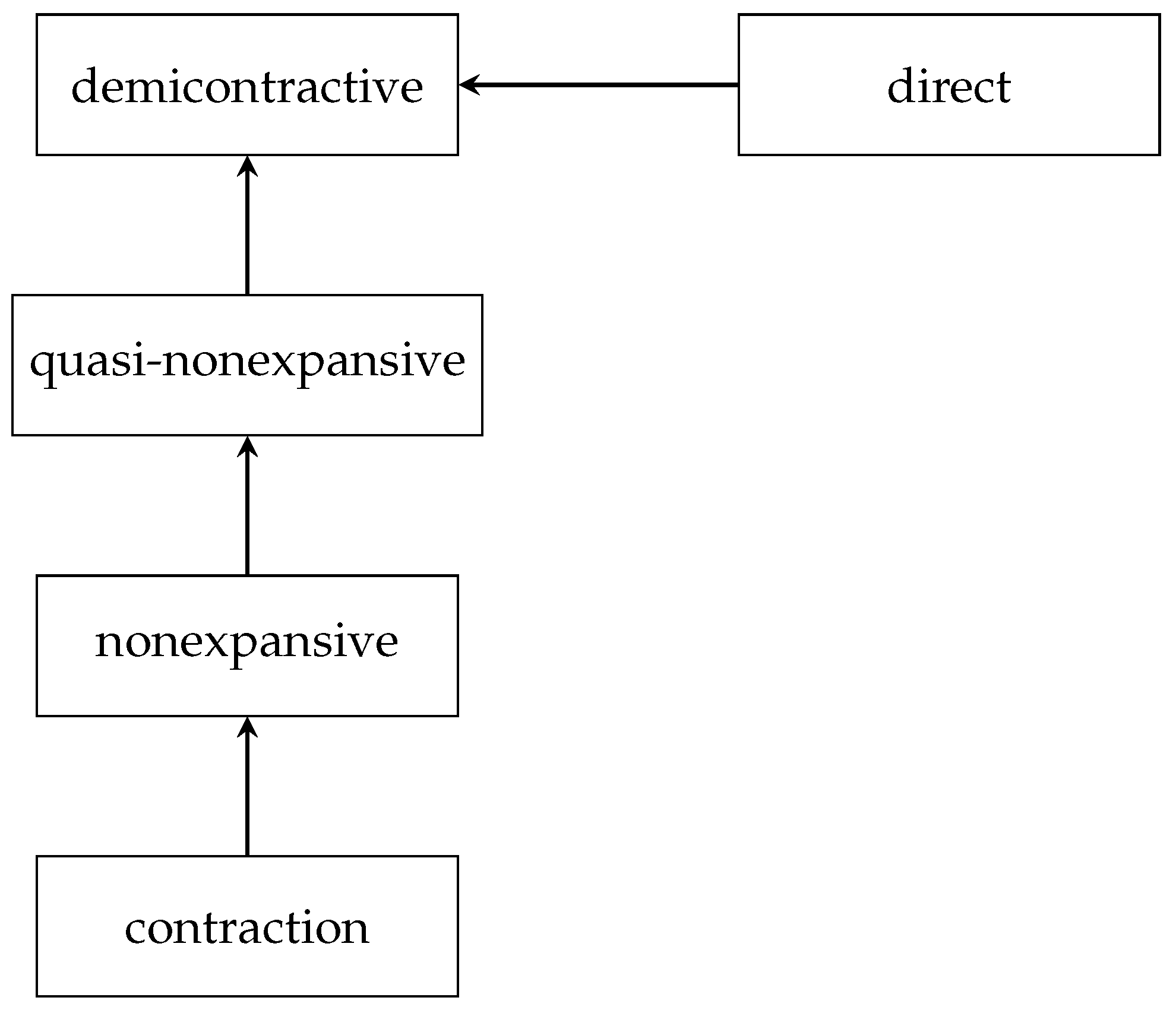
Every contraction operator is nonexpansive;

2. 

Every nonexpansive operator is quasi-nonexpansive;

3. 

Every quasi-nonexpansive operator is 0-demicontractive operator;

4. 

Every direct operator is $-1$-demicontractive operator.

Definition 2.

Assume that $T:H\to H$ is an operator. Then $I-T$ is demiclosed at zero if, for any $\left\{x_n\right\}$ in H, $x_n\rightharpoonup x^{\ast }$ and $(I-T)x_n\to 0$ imply $T{x}^{\ast }=x^{\ast }$.

Remark 3.

Every nonexpansive operator is demiclosed at zero [17].

Definition 3.

Assume that C is a nonempty closed convex subset of H. The metric projection $P_C$ from H onto C is defined as follows: For all $x\in H$,

$$\Vert x-P_{C}x\Vert =inf\{\Vert x-y\Vert :y\in C\}.$$

Note that the metric projection $P_C$ is nonexpansive [17].

Lemma 1

([18]). Assume that C is a nonempty closed convex subset of H and $P_C$ is a nonexpansive operator from H onto C. For any $x\in H$, it satisfies the inequality:

$$\begin{array}{c}\hfill \langle P_{C}x-x,P_{C}x-y\rangle \le 0,\forall y\in C.\end{array}$$

Lemma 2

([19]). Assume that $\left\{{\alpha }_n\right\}$ is a sequence of nonnegative numbers such that

$${\alpha }_{n+1}\le (1-{\beta }_n){\alpha }_n+{\gamma }_n,\forall n\ge 0,$$

where ${\beta }_n\in (0,1)$ and ${\gamma }_n\in \mathbb{R}$ such that

1. 

${\displaystyle \sum _{n=1}^{\infty }}{\beta }_n=\infty$;

2. 

$\underset{n\to \infty }{lim\; sup}\frac{{\gamma }_n}{{\beta }_n}\le 0$ or ${\displaystyle \sum _{n=1}^{\infty }}\left|{\gamma }_n\right|<\infty$.

Then $\underset{n\to \infty }{lim}{\alpha }_n=0$.

Lemma 3

([20]). Assume that $A:H\to H$ is a τ-demicontractive operator with $\tau <1$. Define $U_{\lambda }:=(1-\lambda )I+\lambda U$ for any $\lambda \in (0,1-\tau )$. Then, for any $x\in H$ and $x^{\ast }\in Fix\left(U\right)$,

$$\Vert U_{\lambda }x-x^{\ast }{\Vert }^2\le \Vert x-x^{\ast }{\Vert }^2-\lambda (1-\tau -\lambda ){\Vert x-Ux\Vert }^2.$$

Lemma 4

([14]). Assume that $A:H\to H$ is a bounded linear operator. Assume that $T:H\to H$ is a τ-demicontractive operator. If $A^{-1}(Fix\left(T\right))\ne \varnothing$, then

1. 

$(I-T)Ax=0$ if and only if $A^{\ast }(I-T)Ax=0$ for all $x\in H$;

2. 

In particular, for all $x^{\ast }\in A^{-1}(Fix\left(T\right))$,

$$\begin{array}{c}\hfill \Vert x-\rho A^{\ast }(I-T)Ax-x^{\ast }{\Vert }^2\le {\Vert x-x^{\ast }\Vert }^2-\frac{{(1-\tau )}^2{\Vert (I-T)Ax\Vert }^4}{4\Vert A^{\ast }{(I-T)Ax\Vert }^2},\end{array}$$

where $x\in H$, $Ax\ne T\left(Ax\right)$ and

$$\rho =\frac{{(1-\tau )\Vert (I-T)Ax\Vert }^2}{2\Vert A^{\ast }{(I-T)Ax\Vert }^2}.$$

3. Main Results

Theorem 1.

Assume that $H_1$ and $H_2$ are real Hilbert spaces. Assume that $U:H_1\to H_1$ and $T:H_2\to H_2$ are a κ-demicontractive operator and a τ-demicontractive operator with constants $0\le \kappa <1$ and $0\le \tau <1$, respectively such that $I-U$ and $I-T$ are demiclosed at zero, respectively. Assume that $A:H_1\to H_2$ is a bounded linear operator with the adjoint $A^{\ast }$ of A. Assume that f is a contraction operator with constant η. Assume that S is a set of all solution of the problem (6) such that $S\ne \varnothing$. If $\underset{n\to \infty }{lim}{\alpha }_n=0$, ${\displaystyle \sum _{n=0}^{\infty }}{\alpha }_n=\infty$ and ${\displaystyle \sum _{n=0}^{\infty }}{\beta }_n<\infty$, then the sequence $\left\{x_n\right\}$ generated by algorithm (11) converges strongly to a point $x^{\ast }\in S$, which is a solution $x^{\ast }=P_{S}f\left(x^{\ast }\right)$ of the following variational inequality:

$$\begin{array}{c}\hfill \langle x^{\ast }-f\left(x^{\ast }\right),x^{\ast }-z\rangle \le 0,\forall z\in S.\end{array}$$

(12)

Proof. 

Let $a_n=x_n-{\rho }_n{A}^{\ast }(I-T)A{x}_n$ for each $n\ge 0$ and let $z\in S$. Since ${\beta }_n\in [0,1)$ and ${\displaystyle \sum _{n=0}^{\infty }}{\beta }_n<\infty$, we have $\underset{n\to \infty }{lim}{\beta }_n=0$. For the proof, we have the following four steps:

Step 1. Show that $\left\{x_n\right\}$ is bounded.

Case ${\rho }_n=0$: Thus $a_n=x_n$. By Lemma 3, we get

$$\begin{array}{ccc}\hfill \Vert U_{{\lambda }_n}{a}_n{-z\Vert }^2& =\hfill & \Vert U_{{\lambda }_n}{x}_n{-z\Vert }^2\hfill \\ & \le \hfill & \Vert x_n{-z\Vert }^2-{\lambda }_n(1-\kappa -{\lambda }_n){\Vert x_n-U{x}_n\Vert }^2\hfill \\ & \le \hfill & \Vert x_n{-z\Vert }^2.\hfill \end{array}$$

Case ${\rho }_n\ne 0$: By Lemmas 3 and 4, we get

$$\begin{array}{ccc}\hfill \Vert U_{{\lambda }_n}{a}_n{-z\Vert }^2& \le \hfill & \Vert a_n{-z\Vert }^2-{\lambda }_n(1-\kappa -{\lambda }_n){\Vert a_n-U{a}_n\Vert }^2\hfill \\ & =\hfill & \Vert x_n-{\rho }_n{A}^{\ast }(I-T)A{x}_n{\Vert }^2-{\lambda }_n(1-\kappa -{\lambda }_n){\Vert a_n-U{a}_n\Vert }^2\hfill \\ & \le \hfill & \Vert x_n{-z\Vert }^2-\frac{{(1-\tau )}^2{\Vert (I-T)A{x}_n\Vert }^4}{4\Vert A^{\ast }(I-T)A{x}_n{\Vert }^2}-{\lambda }_n(1-\kappa -{\lambda }_n){\Vert a_n-U{a}_n\Vert }^2\hfill \\ & \le \hfill & \Vert x_n{-z\Vert }^2.\hfill \end{array}$$

Thus $\Vert U_{\lambda }{a}_n-z\Vert \le \Vert x_n-z\Vert$. Observe that

$$\begin{array}{ccc}\hfill \Vert x_{n+1}-z\Vert & =\hfill & \Vert (1-{\beta }_n)y_n+{\beta }_{n}f\left(y_n\right)-z\Vert \hfill \\ & \le \hfill & (1-{\beta }_n)\Vert y_n-z\Vert +{\beta }_n\Vert f\left(y_n\right)-z\Vert \hfill \\ & \le \hfill & (1-{\beta }_n)\Vert y_n-z\Vert +{\beta }_n\Vert f\left(y_n\right)-f\left(z\right)\Vert +{\beta }_n\Vert f\left(z\right)-z\Vert \hfill \\ & \le \hfill & \Vert y_n-z\Vert +{\beta }_n\Vert f\left(z\right)-z\Vert \hfill \\ & =\hfill & \Vert {\alpha }_{n}f\left(x_n\right)+(1-{\alpha }_n)U_{{\lambda }_n}{a}_n-z\Vert +{\beta }_n\Vert f\left(z\right)-z\Vert \hfill \\ & \le \hfill & {\alpha }_n\Vert f\left(x_n\right)-z\Vert +(1-{\alpha }_n)\Vert U_{{\lambda }_n}{a}_n-z\Vert +{\beta }_n\Vert f\left(z\right)-z\Vert \hfill \\ & \le \hfill & {\alpha }_n\Vert f\left(x_n\right)-f\left(z\right)\Vert +{\alpha }_n\Vert f\left(z\right)-z\Vert \hfill \\ & & +(1-{\alpha }_n)\Vert U_{{\lambda }_n}{a}_n-z\Vert +{\beta }_n\Vert f\left(z\right)-z\Vert \hfill \\ & \le \hfill & \eta {\alpha }_n\Vert x_n-z\Vert +{\alpha }_n\Vert f\left(z\right)-z\Vert +(1-{\alpha }_n)\Vert U_{{\lambda }_n}{a}_n-z\Vert +{\beta }_n\Vert f\left(z\right)-z\Vert \hfill \\ & \le \hfill & \eta {\alpha }_n\Vert x_n-z\Vert +{\alpha }_n\Vert f\left(z\right)-z\Vert +(1-{\alpha }_n)\Vert x_n-z\Vert +{\beta }_n\Vert f\left(z\right)-z\Vert \hfill \\ & =\hfill & (1-(1-\eta ){\alpha }_n)\Vert x_n-z\Vert +{\alpha }_n\Vert f\left(z\right)-z\Vert +{\beta }_n\Vert f\left(z\right)-z\Vert \hfill \\ & \le \hfill & max\{\Vert x_n-z\Vert ,\frac{1}{1-\eta }\Vert f\left(z\right)-z\Vert \}+{\beta }_n\Vert f\left(z\right)-z\Vert \hfill \\ & \le \hfill & max\{\Vert x_0-z\Vert ,\frac{1}{1-\eta }\Vert f\left(z\right)-z\Vert \}+\Vert f\left(z\right)-z\Vert {\displaystyle \sum _{n=0}^{\infty }}{\beta }_n.\hfill \end{array}$$

Thus $\left\{x_n\right\}$ is bounded. Moreover, $\left\{f\left(x_n\right)\right\}$, $\left\{y_n\right\}$ and $\left\{f\left(y_n\right)\right\}$ are also bounded.

Step 2. Show that, if the subsequence $\left\{x_{n_k+1}\right\}$ of $\left\{x_n\right\}$ weakly converges to $q\in Fix\left(f\right)$, then the subsequence $\left\{y_{n_k}\right\}$ of $\left\{y_n\right\}$ weakly converges to q. Now, we consider

$$\begin{array}{ccc}\hfill \langle x_{n_k+1}-y_{n_k},q\rangle & =\hfill & {\beta }_{n_k}\langle y_{n_k}-f\left(y_{n_k}\right),q\rangle \hfill \\ & =\hfill & {\beta }_{n_k}\frac{\Vert y_{n_k}-f\left(y_{n_k}\right){+q\Vert }^2+{\Vert y_{n_k}-f\left(y_{n_k}\right)-q\Vert }^2}{4}.\hfill \end{array}$$

Since $\left\{y_n\right\}$ and $\left\{f\left(y_n\right)\right\}$ are bounded, $\left\{y_{n_k}\right\}$ weakly converges to q.

Step 3. Show that the inequality holds:

$$\begin{array}{ccc}\hfill \Vert x_{n+1}-x^{\ast }{\Vert }^2& \le \hfill & (1-{\alpha }_n){\Vert x_n-x^{\ast }\Vert }^2+2{\alpha }_n\langle f\left(x_n\right)-x^{\ast },y_n-x^{\ast }\rangle \hfill \\ & & +2{\beta }_n\Vert y_n-x^{\ast }\Vert \Vert f\left(x^{\ast }\right)-x^{\ast }\Vert +{\beta }_n^2{\Vert f\left(x^{\ast }\right)-x^{\ast }\Vert }^2.\hfill \end{array}$$

Case ${\rho }_n=0$: By Lemma 3, we get

$$\begin{array}{ccc}\hfill \Vert x_{n+1}-x^{\ast }{\Vert }^2& =\hfill & \Vert (1-{\beta }_n)y_n+{\beta }_{n}f\left(y_n\right)-x^{\ast }{\Vert }^2\hfill \\ & \le \hfill & ((1-{\beta }_n)\Vert y_n-x^{\ast }\Vert +{\beta }_n\Vert f\left(y_n\right)-x^{\ast }{\Vert )}^2\hfill \\ & \le \hfill & ((1-{\beta }_n)\Vert y_n-x^{\ast }\Vert +{\beta }_n\Vert f\left(y_n\right)-f\left(x^{\ast }\right)\Vert +{\beta }_n\Vert f\left(x^{\ast }\right)-x^{\ast }{\Vert )}^2\hfill \\ & \le \hfill & (\Vert y_n-x^{\ast }\Vert +{\beta }_n\Vert f\left(x^{\ast }\right)-x^{\ast }{\Vert )}^2\hfill \\ & =\hfill & \Vert y_n-x^{\ast }{\Vert }^2+2{\beta }_n\Vert y_n-x^{\ast }\Vert \Vert f\left(x^{\ast }\right)-x^{\ast }\Vert +{\beta }_n^2{\Vert f\left(x^{\ast }\right)-x^{\ast }\Vert }^2\hfill \\ & =\hfill & \Vert {\alpha }_{n}f\left(x_n\right)+(1-{\alpha }_n)U_{{\lambda }_n}{x}_n-x^{\ast }{\Vert }^2\hfill \\ & & +2{\beta }_n\Vert y_n-x^{\ast }\Vert \Vert f\left(x^{\ast }\right)-x^{\ast }\Vert +{\beta }_n^2{\Vert f\left(x^{\ast }\right)-x^{\ast }\Vert }^2\hfill \\ & =\hfill & \Vert {\alpha }_n(f\left(x_n\right)-x^{\ast })+(1-{\alpha }_n)(U_{{\lambda }_n}{x}_n-x^{\ast }){\Vert }^2\hfill \\ & & +2{\beta }_n\Vert y_n-x^{\ast }\Vert \Vert f\left(x^{\ast }\right)-x^{\ast }\Vert +{\beta }_n^2{\Vert f\left(x^{\ast }\right)-x^{\ast }\Vert }^2\hfill \\ & \le \hfill & {(1-{\alpha }_n)}^2{\Vert U_{{\lambda }_n}{x}_n-x^{\ast }\Vert }^2+2{\alpha }_n\langle f\left(x_n\right)-x^{\ast },y_n-x^{\ast }\rangle \hfill \\ & & +2{\beta }_n\Vert y_n-x^{\ast }\Vert \Vert f\left(x^{\ast }\right)-x^{\ast }\Vert +{\beta }_n^2{\Vert f\left(x^{\ast }\right)-x^{\ast }\Vert }^2\hfill \\ & \le \hfill & {(1-{\alpha }_n)}^2(\Vert x_n-x^{\ast }{\Vert }^2-{\lambda }_n(1-\kappa -{\lambda }_n)\Vert x_n-U{x}_n{\Vert }^2)\hfill \\ & & +2{\alpha }_n\langle f\left(x_n\right)-x^{\ast },y_n-x^{\ast }\rangle +{\beta }_n^2{\Vert f\left(x^{\ast }\right)-x^{\ast }\Vert }^2\hfill \\ & & +2{\beta }_n\Vert y_n-x^{\ast }\Vert \Vert f\left(x^{\ast }\right)-x^{\ast }\Vert .\hfill \end{array}$$

Case ${\rho }_n\ne 0$: By Lemmas 3 and 4, we get

$$\begin{array}{ccc}\hfill \Vert x_{n+1}-x^{\ast }{\Vert }^2& =\hfill & \Vert (1-{\beta }_n)y_n+{\beta }_{n}f\left(y_n\right)-x^{\ast }{\Vert }^2\hfill \\ & \le \hfill & ((1-{\beta }_n)\Vert y_n-x^{\ast }\Vert +{\beta }_n\Vert f\left(y_n\right)-x^{\ast }{\Vert )}^2\hfill \\ & \le \hfill & ((1-{\beta }_n)\Vert y_n-x^{\ast }\Vert +{\beta }_n\Vert f\left(y_n\right)-f\left(x^{\ast }\right)\Vert +{\beta }_n\Vert f\left(x^{\ast }\right)-x^{\ast }{\Vert )}^2\hfill \\ & \le \hfill & \Vert y_n-x^{\ast }{\Vert }^2+2{\beta }_n\Vert y_n-x^{\ast }\Vert \Vert f\left(x^{\ast }\right)-x^{\ast }\Vert +{\beta }_n^2{\Vert f\left(x^{\ast }\right)-x^{\ast }\Vert }^2\hfill \\ & =\hfill & \Vert {\alpha }_{n}f\left(x_n\right)+(1-{\alpha }_n)U_{{\lambda }_n}{a}_n-x^{\ast }{\Vert }^2\hfill \\ & & +2{\beta }_n\Vert y_n-x^{\ast }\Vert \Vert f\left(x^{\ast }\right)-x^{\ast }\Vert +{\beta }_n^2{\Vert f\left(x^{\ast }\right)-x^{\ast }\Vert }^2\hfill \\ & =\hfill & \Vert {\alpha }_n(f\left(x_n\right)-x^{\ast })+(1-{\alpha }_n)(U_{{\lambda }_n}{a}_n-x^{\ast }){\Vert }^2\hfill \\ & & +2{\beta }_n\Vert y_n-x^{\ast }\Vert \Vert f\left(x^{\ast }\right)-x^{\ast }\Vert +{\beta }_n^2{\Vert f\left(x^{\ast }\right)-x^{\ast }\Vert }^2\hfill \\ & \le \hfill & {(1-{\alpha }_n)}^2{\Vert U_{{\lambda }_n}{a}_n-x^{\ast }\Vert }^2+2{\alpha }_n\langle f\left(x_n\right)-x^{\ast },y_n-x^{\ast }\rangle \hfill \\ & & +2{\beta }_n\Vert y_n-x^{\ast }\Vert \Vert f\left(x^{\ast }\right)-x^{\ast }\Vert +{\beta }_n^2{\Vert f\left(x^{\ast }\right)-x^{\ast }\Vert }^2\hfill \\ & \le \hfill & {(1-\alpha )}^2(\Vert a_n-x^{\ast }{\Vert }^2-{\lambda }_n(1-\kappa -{\lambda }_n)\Vert a_n-U{a}_n{\Vert }^2)\hfill \\ & & +2{\alpha }_n\langle f\left(x_n\right)-x^{\ast },y_n-x^{\ast }\rangle +{\beta }_n^2{\Vert f\left(x^{\ast }\right)-x^{\ast }\Vert }^2\hfill \\ & & +2{\beta }_n\Vert y_n-x^{\ast }\Vert \Vert f\left(x^{\ast }\right)-x^{\ast }\Vert \hfill \\ & \le \hfill & {(1-\alpha )}^2(\Vert x_n-x^{\ast }{\Vert }^2-\frac{{(1-\tau )}^2{\Vert (I-T)A{x}_n\Vert }^4}{4\Vert A^{\ast }(I-T)A{x}_n{\Vert }^2}\hfill \\ & & -{\lambda }_n(1-\kappa -{\lambda }_n)\Vert a_n-U{a}_n{\Vert }^2)\hfill \\ & & +2{\alpha }_n\langle f\left(x_n\right)-x^{\ast },y_n-x^{\ast }\rangle +{\beta }_n^2{\Vert f\left(x^{\ast }\right)-x^{\ast }\Vert }^2\hfill \\ & & +2{\beta }_n\Vert y_n-x^{\ast }\Vert \Vert f\left(x^{\ast }\right)-x^{\ast }\Vert .\hfill \end{array}$$

Therefore, we have

$$\begin{gathered} \Vert x_{n+1}-x^{\ast }{\Vert }^2\le (1-{\alpha }_n)\Vert x_n-x^{\ast }{\Vert }^2+2{\alpha }_n\langle f\left(x_n\right)-x^{\ast },y_n-x^{\ast }\rangle \\ \hspace{1em}\hspace{1em}+2{\beta }_n\Vert y_n-x^{\ast }\Vert \Vert f\left(x^{\ast }\right)-x^{\ast }\Vert +{\beta }_n^2{\Vert f\left(x^{\ast }\right)-x^{\ast }\Vert }^2. \end{gathered}$$

Step 4. Show that $x_n\to x^{\ast }$ for each $n\ge 0$. Let $s_n=\Vert x_n-x^{\ast }\Vert$. In this step, we consider two cases.

Case 1. Assume that there is $n_0\in \mathbb{N}$ such that $\left\{s_n\right\}$ is decreasing for all $n\ge n_0$. Since $\left\{s_n\right\}$ is monotonic and bounded, $\left\{s_n\right\}$ is convergent. First, we show that

$$\underset{n\to \infty }{lim\; sup}\langle f\left(x^{\ast }\right)-x^{\ast },y_n-x^{\ast }\rangle \le 0.$$

There are two parts to show this.

Part 1. Let ${\rho }_n=0$. Since $\left\{f\left(x_n\right)\right\}$ and $\left\{y_n\right\}$ are bounded and Step 3, we get

$$\begin{array}{c}\hfill {\lambda }_n(1-\kappa -{\lambda }_n){\Vert x_n-U{x}_n\Vert }^2\le s_n-s_{n+1}+{\alpha }_{n}M+{\beta }_{n}N,\end{array}$$

where

$$M=\underset{n\in \mathbb{N}}{sup}\left\{2\langle f\left(x_n\right)-x^{\ast },y_n-x^{\ast }\rangle \right\}$$

and

$$N=\underset{n\in \mathbb{N}}{sup}\{2\Vert y_n-x^{\ast }\Vert \Vert f\left(x^{\ast }\right)-x^{\ast }\Vert +{\beta }_n\Vert f\left(x^{\ast }\right)-x^{\ast }{\Vert }^2\}.$$

Since $\left\{s_n\right\}$ is convergent and $\underset{n\to \infty }{lim}{\alpha }_n=0$, we have $\underset{n\to \infty }{lim}\Vert x_n-U{x}_n\Vert =0$. By since ${\rho }_n=0$, we have

$$\underset{n\to \infty }{lim}\Vert (I-T)A{x}_n\Vert =0.$$

By the boundedness of $\left\{x_n\right\}$, there is a subsequence $\left\{x_{n_k}\right\}$ of $\left\{x_n\right\}$ such that $x_{n_k}\rightharpoonup q$ and

$$\begin{array}{ccc}\hfill \underset{n\to \infty }{lim\; sup}\langle f\left(x^{\ast }\right)-x^{\ast },x_n-x^{\ast }\rangle & =\hfill & \underset{k\to \infty }{lim}\langle f\left(x^{\ast }\right)-x^{\ast },x_{n_k}-x^{\ast }\rangle \hfill \\ & =\hfill & \langle f\left(x^{\ast }\right)-x^{\ast },q-x^{\ast }\rangle .\hfill \end{array}$$

Since $\underset{n\to \infty }{lim}\Vert x_n-U{x}_n\Vert =0$ and the demiclosedness of $I-U$ at zero, we have $q\in Fix\left(U\right)$. Since A is a bounded linear operator, A is continuous. Therefore, $x_{n_k}\rightharpoonup q$ imply $A{x}_{n_k}\rightharpoonup Aq$. Form $\underset{n\to \infty }{lim}\Vert (I-T)A{x}_n\Vert =0$ and the demiclosedness of $I-T$ at zero, it follows that $Aq\in Fix\left(T\right)$ and so $q\in S$. By Step 2, it follows that

$$\begin{array}{ccc}\hfill 0& \ge \hfill & \langle f\left(x^{\ast }\right)-x^{\ast },q-x^{\ast }\rangle =\underset{k\to \infty }{lim}\langle f\left(x^{\ast }\right)-x^{\ast },x_{n_k}-x^{\ast }\rangle \hfill \\ & =\hfill & \underset{n\to \infty }{lim\; sup}\langle f\left(x^{\ast }\right)-x^{\ast },x_n-x^{\ast }\rangle \hfill \\ & =\hfill & \underset{n\to \infty }{lim\; sup}\langle f\left(x^{\ast }\right)-x^{\ast },y_{n-1}-x^{\ast }\rangle .\hfill \end{array}$$

Part 2. Let ${\rho }_n\ne 0$. Since $\left\{f\left(x_n\right)\right\}$ and $\left\{y_n\right\}$ are bounded, by Step 3, we get

$$\begin{array}{c}\hfill {\lambda }_n(1-\kappa -{\lambda }_n){\Vert a_n-U{a}_n\Vert }^2+\frac{{(1-\tau )}^2{\Vert (I-T)A{x}_n\Vert }^4}{4\Vert A^{\ast }(I-T)A{x}_n{\Vert }^2}\le s_n-s_{n+1}+{\alpha }_{n}M+{\beta }_{n}N,\end{array}$$

where

$$M=\underset{n\in \mathbb{N}}{sup}\left\{2\langle f\left(x_n\right)-x^{\ast },y_n-x^{\ast }\rangle \right\}$$

and

$$N=\underset{n\in \mathbb{N}}{sup}\{2\Vert y_n-x^{\ast }\Vert \Vert f\left(x^{\ast }\right)-x^{\ast }\Vert +{\beta }_n\Vert f\left(x^{\ast }\right)-x^{\ast }{\Vert }^2\}.$$

Thus we obtain

$$\begin{array}{c}0\le {\lambda }_n(1-\kappa -{\lambda }_n){\Vert a_n-U{a}_n\Vert }^2\le s_n-s_{n+1}+{\alpha }_{n}M+{\beta }_{n}N\end{array}$$

and

$$\begin{array}{c}0\le \frac{{(1-\tau )}^2{\Vert (I-T)A{x}_n\Vert }^4}{4\Vert A^{\ast }(I-T)A{x}_n{\Vert }^2}\le s_n-s_{n+1}+{\alpha }_{n}M+{\beta }_{n}N.\end{array}$$

Since $\left\{s_n\right\}$ is convergent and $\underset{n\to \infty }{lim}{\alpha }_n=0$, we obtain

$$\begin{array}{c}\hfill \underset{n\to \infty }{lim}\Vert a_n-U{a}_n\Vert =\underset{n\to \infty }{lim}\frac{\Vert (I-T)A{x}_n{\Vert }^4}{\Vert A^{\ast }(I-T)A{x}_n{\Vert }^2}=0.\end{array}$$

Moreover, we get $\underset{n\to \infty }{lim}\Vert (I-T)A{x}_n\Vert =0$. However, it follows that

$$\begin{array}{c}\Vert (I-T)A{x}_n\Vert =\Vert A\Vert \Vert (I-T)A{x}_n{\Vert }^2\frac{1}{\Vert A\Vert \Vert (I-T)A{x}_n\Vert }\le \Vert A\Vert \frac{\Vert (I-T)A{x}_n{\Vert }^2}{\Vert A^{\ast }(I-T)A{x}_n\Vert }.\hfill \end{array}$$

Thus we have

$$\underset{n\to \infty }{lim}\Vert x_n-a_n\Vert =\underset{n\to \infty }{lim}\frac{(1-\tau )\Vert (I-T)A{x}_n{\Vert }^2}{2\Vert A^{\ast }(I-T)A{x}_n\Vert }=0.$$

By the boundedness of $\left\{x_n\right\}$, there is a subsequence $\left\{x_{n_k}\right\}$ of $\left\{x_n\right\}$ such that $x_{n_k}\rightharpoonup q$. Since $\underset{n\to \infty }{lim}\Vert x_n-a_n\Vert =0$ and $x_{n_k}\rightharpoonup q$, there is a subsequence $\left\{a_{n_k}\right\}$ of $\left\{a_n\right\}$ such that $a_{n_k}\rightharpoonup q$ and

$$\begin{array}{c}\underset{n\to \infty }{lim\; sup}\langle f\left(x^{\ast }\right)-x^{\ast },x_n-x^{\ast }\rangle =\underset{k\to \infty }{lim}\langle f\left(x^{\ast }\right)-x^{\ast },x_{n_k}-x^{\ast }\rangle =\langle f\left(x^{\ast }\right)-x^{\ast },q-x^{\ast }\rangle .\hfill \end{array}$$

Since $\underset{n\to \infty }{lim}\Vert a_n-U{a}_n\Vert =0$, by the demiclosedness of $I-U$ at zero, we have $q\in Fix\left(U\right)$. Since A is a bounded linear operator, A is continuous. Therefore, $x_{n_k}\rightharpoonup q$ imply $A{x}_{n_k}\rightharpoonup Aq$. Form $\underset{n\to \infty }{lim}\Vert (I-T)A{x}_n\Vert =0$ and the demiclosedness of $I-T$ at zero, we have $Aq\in Fix\left(T\right)$ and $q\in S$. By Step 2, it follow that

$$\begin{array}{ccc}\hfill 0& \ge \hfill & \langle f\left(x^{\ast }\right)-x^{\ast },q-x^{\ast }\rangle =\underset{k\to \infty }{lim}\langle f\left(x^{\ast }\right)-x^{\ast },x_{n_k}-x^{\ast }\rangle \hfill \\ & =\hfill & \underset{n\to \infty }{lim\; sup}\langle f\left(x^{\ast }\right)-x^{\ast },x_n-x^{\ast }\rangle \hfill \\ & =\hfill & \underset{n\to \infty }{lim\; sup}\langle f\left(x^{\ast }\right)-x^{\ast },y_{n-1}-x^{\ast }\rangle .\hfill \end{array}$$

Second, we show that $\underset{n\to \infty }{lim}\Vert x_{n+1}-x_n\Vert =0$. There are two parts.

Part 1. If ${\rho }_n=0$, then we get

$$\begin{array}{ccc}\hfill \Vert x_{n+1}-x_n\Vert & =\hfill & \Vert (1-{\beta }_n)y_n+{\beta }_{n}f\left(y_n\right)-x_n\Vert \hfill \\ & \le \hfill & (1-{\beta }_n)\Vert y_n-x_n\Vert +{\beta }_n\Vert f\left(y_n\right)-x_n\Vert \hfill \\ & =\hfill & (1-{\beta }_n)\Vert {\alpha }_{n}f\left(x_n\right)+(1-{\alpha }_n)U_{{\lambda }_n}{x}_n-x_n\Vert +{\beta }_n\Vert f\left(y_n\right)-x_n\Vert \hfill \\ & \le \hfill & {\alpha }_n\Vert f\left(x_n\right)-x_n\Vert +(1-{\alpha }_n)\Vert x_n-U_{{\lambda }_n}{x}_n\Vert +{\beta }_n\Vert f\left(y_n\right)-x_n\Vert \hfill \\ & =\hfill & {\alpha }_n\Vert f\left(x_n\right)-x_n\Vert +{\lambda }_n\Vert x_n-U{x}_n\Vert +{\beta }_n\Vert f\left(y_n\right)-x_n\Vert .\hfill \end{array}$$

Part 2. If ${\rho }_n\ne 0$, then we get

$$\begin{array}{ccc}\hfill \Vert x_{n+1}-x_n\Vert & \le \hfill & \Vert (1-{\beta }_n)y_n+{\beta }_{n}f\left(y_n\right)-x_n\Vert \hfill \\ & \le \hfill & (1-{\beta }_n)\Vert y_n-x_n\Vert +{\beta }_n\Vert f\left(y_n\right)-x_n\Vert \hfill \\ & =\hfill & (1-{\beta }_n)\Vert {\alpha }_{n}f\left(x_n\right)+(1-{\alpha }_n)U_{{\lambda }_n}{a}_n-x_n\Vert +{\beta }_n\Vert f\left(y_n\right)-x_n\Vert \hfill \\ & \le \hfill & {\alpha }_n\Vert f\left(x_n\right)-x_n\Vert +(1-{\alpha }_n)\Vert x_n-U_{{\lambda }_n}{a}_n\Vert +{\beta }_n\Vert f\left(y_n\right)-x_n\Vert \hfill \\ & \le \hfill & {\alpha }_n\Vert f\left(x_n\right)-x_n\Vert +\Vert x_n-a_n\Vert +\Vert a_n-U_{{\lambda }_n}{a}_n\Vert +{\beta }_n\Vert f\left(y_n\right)-x_n\Vert \hfill \\ & =\hfill & {\alpha }_n\Vert f\left(x_n\right)-x_n\Vert +\Vert x_n-a_n\Vert +{\lambda }_n\Vert a_n-U{a}_n\Vert +{\beta }_n\Vert f\left(y_n\right)-x_n\Vert .\hfill \end{array}$$

Therefore, we have $\underset{n\to \infty }{lim}\Vert x_{n+1}-x_n\Vert =0$.

Third, we show that $x_n\to x^{\ast }$. We get the inequality:

$$\underset{n\to \infty }{lim\; sup}\langle f\left(x^{\ast }\right)-x^{\ast },y_n-x^{\ast }\rangle \le 0.$$

Now, we have

$$\begin{gathered} \Vert x_{n+1}-x^{\ast }{\Vert }^2\le (1-{\alpha }_n)\Vert x_n-x^{\ast }{\Vert }^2+2{\alpha }_n\underset{k\to \infty }{lim\; sup}\langle f\left(x_k\right)-x^{\ast },y_k-x^{\ast }\rangle \\ \hspace{1em}+{\beta }_n\underset{k\in \mathbb{N}}{sup}\{2\Vert y_k-x^{\ast }\Vert \Vert f\left(x^{\ast }\right)-x^{\ast }\Vert +{\beta }_k\Vert f\left(x^{\ast }\right)-x^{\ast }{\Vert }^2\}. \end{gathered}$$

By Lemma 2, we have $\underset{n⟶\infty }{lim}{s}_n=\underset{n⟶\infty }{lim}\Vert x_n-x^{\ast }\Vert =0$ and so $x_n\to x^{\ast }$.

Case 2. Assume that there is not $n_0\in \mathbb{N}$ such that $\left\{s_n\right\}$ is decreasing for all $n\ge n_0$. Thus there is a subsequence $\left\{s_{n_i+1}\right\}$ of $\left\{s_n\right\}$ such that $s_{n_i+1}<s_{n_{i+1}+1}$ for all $i\in \mathbb{N}$.

First, we show that

$$\underset{n_i\to \infty }{lim\; sup}\langle f\left(x^{\ast }\right)-x^{\ast },y_{n_i}-x^{\ast }\rangle \le 0.$$

There are two parts.

Part 1. Let ${\rho }_{n_i}=0$. Since $\left\{f\left(x_{n_i}\right)\right\}$ and $\left\{y_{n_i}\right\}$ are bounded, by Step 3, we get

$$\begin{array}{c}{\lambda }_{n_i}(1-\kappa -{\lambda }_{n_i}){\Vert x_{n_i}-U{x}_{n_i}\Vert }^2\le s_{n_i}-s_{n_{i+1}}+{\alpha }_{n_i}M+{\beta }_{n_i}N\le {\alpha }_{n_i}M+{\beta }_{n_i}N,\hfill \end{array}$$

where

$$M\in \mathbb{R}=\underset{n_i\in \mathbb{N}}{sup}\left\{2\langle f\left(x_{n_i}\right)-x^{\ast },y_{n_i}-x^{\ast }\rangle \right\}$$

and

$$N=\underset{n\in \mathbb{N}}{sup}\{2\Vert y_{n_i}-x^{\ast }\Vert \Vert f\left(x^{\ast }\right)-x^{\ast }\Vert +{\beta }_{n_i}\Vert f\left(x^{\ast }\right)-x^{\ast }{\Vert }^2\}.$$

Since $\underset{i\to \infty }{lim}{\alpha }_{n_i}=0$, we have

$$\underset{i\to \infty }{lim}\Vert x_{n_i}-U{x}_{n_i}\Vert =0.$$

Since ${\rho }_{n_i}=0$, we have

$$\underset{i\to \infty }{lim}\Vert (I-TA)x_{n_i}\Vert =0.$$

By the boundedness of $\left\{x_{n_i}\right\}$, there is a subsequence $\left\{x_{n_{i_j}}\right\}$ of $\left\{x_{n_i}\right\}$ such that $x_{n_{i_j}}\rightharpoonup q$ and

$$\begin{array}{c}\underset{i\to \infty }{lim\; sup}\langle f\left(x^{\ast }\right)-x^{\ast },x_{n_i}-x^{\ast }\rangle =\underset{j\to \infty }{lim}\langle f\left(x^{\ast }\right)-x^{\ast },x_{n_{i_j}}-x^{\ast }\rangle =\langle f\left(x^{\ast }\right)-x^{\ast },q-x^{\ast }\rangle .\hfill \end{array}$$

Since $\underset{j\to \infty }{lim}\Vert x_{n_{i_j}}-U{x}_{n_{i_j}}\Vert =0$ and the demiclosedness of $I-U$ at zero, we have $q\in Fix\left(U\right)$. Since A is a bounded linear operator, A is continuous. Therefore, $x_{n_{i_j}}\rightharpoonup q$ imply $A{x}_{n_{i_j}}\rightharpoonup Aq$. Form $\underset{j\to \infty }{lim}\Vert (I-T)A{x}_{n_{i_j}}\Vert =0$ and the demiclosedness of $I-T$ at zero, we have $Aq\in Fix\left(T\right)$ and so $q\in S$. By Step 2, it follows that

$$\begin{array}{ccc}\hfill 0& \ge \hfill & \langle f\left(x^{\ast }\right)-x^{\ast },q-x^{\ast }\rangle =\underset{j\to \infty }{lim}\langle f\left(x^{\ast }\right)-x^{\ast },x_{n_{i_j}}-x^{\ast }\rangle \hfill \\ & =\hfill & \underset{i\to \infty }{lim\; sup}\langle f\left(x^{\ast }\right)-x^{\ast },x_{n_i}-x^{\ast }\rangle \hfill \\ & =\hfill & \underset{i\to \infty }{lim\; sup}\langle f\left(x^{\ast }\right)-x^{\ast },y_{n_i-1}-x^{\ast }\rangle .\hfill \end{array}$$

Part 2. Let ${\rho }_{n_i}\ne 0$. Since $\left\{f\left(x_{n_i}\right)\right\}$ and $\left\{y_{n_i}\right\}$ are bounded, by Step 3, we get

$$\begin{gathered} {\lambda }_{n_i}(1-\kappa -{\lambda }_{n_i}){\Vert a_{n_i}-U{a}_{n_i}\Vert }^2+\frac{{(1-\tau )}^2{\Vert (I-T)A{x}_{n_i}\Vert }^4}{4\Vert A^{\ast }(I-T)A{x}_{n_i}{\Vert }^2} \\ \le s_{n_i}-s_{n_{i+1}}+{\alpha }_{n_i}M+{\beta }_{n_i}N \\ \le {\alpha }_{n_i}M+{\beta }_{n_i}N, \end{gathered}$$

where

$$M=\underset{n_i\in \mathbb{N}}{sup}\left\{2\langle f\left(x_{n_i}\right)-x^{\ast },y_{n_i}-x^{\ast }\rangle \right\}$$

and

$$N=\underset{n\in \mathbb{N}}{sup}\{2\Vert y_{n_i}-x^{\ast }\Vert \Vert f\left(x^{\ast }\right)-x^{\ast }\Vert +{\beta }_{n_i}\Vert f\left(x^{\ast }\right)-x^{\ast }{\Vert }^2\}.$$

Then we obtain

$$\begin{array}{c}0\le {\lambda }_{n_i}(1-\kappa -{\lambda }_{n_i}){\Vert a_{n_i}-U{a}_{n_i}\Vert }^2\le {\alpha }_{n_i}M+{\beta }_{n_i}N\end{array}$$

and

$$\begin{array}{c}0\le \frac{{(1-\tau )}^2{\Vert (I-T)A{x}_{n_i}\Vert }^4}{4\Vert A^{\ast }(I-T)A{x}_{n_i}{\Vert }^2}\le {\alpha }_{n_i}M+{\beta }_{n_i}N.\end{array}$$

Since $\underset{i\to \infty }{lim}{\alpha }_{n_i}=0$, we obtain

$$\begin{array}{c}\hfill \underset{i\to \infty }{lim}\Vert a_{n_i}-U{a}_{n_i}\Vert =\underset{i\to \infty }{lim}\frac{\Vert (I-T)A{x}_{n_i}{\Vert }^4}{\Vert A^{\ast }(I-T)A{x}_{n_i}{\Vert }^2}=0.\end{array}$$

Moreover, we get $\underset{n\to \infty }{lim}\Vert (I-T)A{x}_{n_i}\Vert =0$. However, we have

$$\begin{array}{c}\Vert (I-T)A{x}_{n_i}\Vert =\Vert A\Vert \Vert (I-T)A{x}_{n_i}{\Vert }^2\frac{1}{\Vert A\Vert \Vert (I-T)A{x}_{n_i}\Vert }\le \Vert A\Vert \frac{\Vert (I-T)A{x}_{n_i}{\Vert }^2}{\Vert A^{\ast }(I-T)A{x}_{n_i}\Vert }.\hfill \end{array}$$

Thus we have

$$\underset{i\to \infty }{lim}\Vert x_{n_i+1}-a_{n_i}\Vert =\underset{i\to \infty }{lim}\frac{(1-\tau )\Vert (I-T)A{x}_{n_i}{\Vert }^2}{2\Vert A^{\ast }(I-T)A{x}_{n_i}\Vert }=0.$$

By the boundedness of $\left\{x_{n_i}\right\}$, there is a subsequence $\left\{x_{n_{i_j}}\right\}$ of $\left\{x_{n_i}\right\}$ and $x_{n_{i_j}}\rightharpoonup q$. Since $\underset{i\to \infty }{lim}\Vert x_{n_i}-a_{n_i}\Vert =0$ and $x_{n_{i_j}}\rightharpoonup q$, we have $a_{n_{i_j}}\rightharpoonup q$ such that

$$\begin{array}{c}\underset{i\to \infty }{lim\; sup}\langle f\left(x^{\ast }\right)-x^{\ast },x_{n_i}-x^{\ast }\rangle =\underset{j\to \infty }{lim}\langle f\left(x^{\ast }\right)-x^{\ast },x_{n_{i_j}}-x^{\ast }\rangle =\langle f\left(x^{\ast }\right)-x^{\ast },q-x^{\ast }\rangle .\hfill \end{array}$$

Since $\underset{i\to \infty }{lim}\Vert a_{n_i}-U{a}_{n_i}\Vert =0$, by the demiclosedness of $I-U$ at zero, we have $q\in Fix\left(U\right)$. Since A is a bounded linear operator, A is continuous. Therefore, $x_{n_{i_j}}\rightharpoonup q$ imply $A{x}_{n_{i_j}}\rightharpoonup Aq$. Form $\underset{i\to \infty }{lim}\Vert (I-T)A{x}_{n_i}\Vert =0$ and the demiclosedness of $I-T$ at zero, we have $Aq\in Fix\left(T\right)$ and so $q\in S$. By Step 2, it follows that

$$\begin{array}{ccc}\hfill 0& \ge \hfill & \langle f\left(x^{\ast }\right)-x^{\ast },q-x^{\ast }\rangle =\underset{j\to \infty }{lim}\langle f\left(x^{\ast }\right)-x^{\ast },x_{n_{i_j}}-x^{\ast }\rangle \hfill \\ & =\hfill & \underset{i\to \infty }{lim\; sup}\langle f\left(x^{\ast }\right)-x^{\ast },x_{n_i}-x^{\ast }\rangle \hfill \\ & =\hfill & \underset{i\to \infty }{lim\; sup}\langle f\left(x^{\ast }\right)-x^{\ast },y_{n_i-1}-x^{\ast }\rangle .\hfill \end{array}$$

Second, we show that

$$\underset{i\to \infty }{lim}\Vert x_{n_{i+1}}-x_{n_i}\Vert =0.$$

There are two parts.

Part 1. If ${\rho }_{n_i}=0$, then we compute

$$\begin{array}{ccc}\hfill \Vert x_{n_{i+1}}-x_{n_i}\Vert & \le \hfill & \Vert (1-{\beta }_{n_i})y_{n_i}+{\beta }_{n_i}f\left(y_{n_i}\right)-x_{n_i}\Vert \hfill \\ & \le \hfill & (1-{\beta }_{n_i})\Vert y_{n_i}-x_{n_i}\Vert +{\beta }_{n_i}\Vert f\left(y_{n_i}\right)-x_{n_i}\Vert \hfill \\ & =\hfill & (1-{\beta }_{n_i})\Vert {\alpha }_{n_i}f\left(x_{n_i}\right)+(1-{\alpha }_{n_i})U_{{\lambda }_{n_i}}{x}_{n_i}-x_{n_i}\Vert +{\beta }_{n_i}\Vert f\left(y_{n_i}\right)-x_{n_i}\Vert \hfill \\ & \le \hfill & {\alpha }_{n_i}\Vert f\left(x_{n_i}\right)-x_{n_i}\Vert +(1-{\alpha }_{n_i})\Vert x_{n_i}-U_{{\lambda }_{n_i}}{x}_{n_i}\Vert +{\beta }_{n_i}\Vert f\left(y_{n_i}\right)-x_{n_i}\Vert \hfill \\ & =\hfill & {\alpha }_{n_i}\Vert f\left(x_{n_i}\right)-x_{n_i}\Vert +{\lambda }_{n_i}\Vert x_{n_i}-U{x}_{n_i}\Vert +{\beta }_{n_i}\Vert f\left(y_{n_i}\right)-x_{n_i}\Vert .\hfill \end{array}$$

Part 2. If ${\rho }_{n_i}\ne 0$, then we compute

$$\begin{array}{ccc}\hfill \Vert x_{n_{i+1}}-x_{n_i}\Vert & \le \hfill & \Vert (1-{\beta }_{n_i})y_{n_i}+{\beta }_{n_i}f\left(y_{n_i}\right)-x_{n_i}\Vert \hfill \\ & \le \hfill & (1-{\beta }_{n_i})\Vert y_{n_i}-x_{n_i}\Vert +{\beta }_{n_i}\Vert f\left(y_{n_i}\right)-x_{n_i}\Vert \hfill \\ & =\hfill & (1-{\beta }_{n_i})\Vert {\alpha }_{n_i}f\left(x_{n_i}\right)+(1-{\alpha }_{n_i})U_{{\lambda }_{n_i}}{a}_{n_i}-x_{n_i}\Vert +{\beta }_{n_i}\Vert f\left(y_{n_i}\right)-x_{n_i}\Vert \hfill \\ & \le \hfill & {\alpha }_{n_i}\Vert f\left(x_{n_i}\right)-x_{n_i}\Vert +(1-{\alpha }_{n_i})\Vert x_{n_i}-U_{{\lambda }_{n_i}}{a}_{n_i}\Vert +{\beta }_{n_i}\Vert f\left(y_{n_i}\right)-x_{n_i}\Vert \hfill \\ & \le \hfill & {\alpha }_{n_i}\Vert f\left(x_{n_i}\right)-x_{n_i}\Vert +\Vert x_{n_i}-a_{n_i}\Vert +\Vert a_{n_i}-U_{{\lambda }_n}{a}_{n_i}\Vert +{\beta }_{n_i}\Vert f\left(y_{n_i}\right)-x_{n_i}\Vert \hfill \\ & =\hfill & {\alpha }_{n_i}\Vert f\left(x_{n_i}\right)-x_{n_i}\Vert +\Vert x_{n_i}-a_{n_i}\Vert +{\lambda }_{n_i}\Vert a_{n_i}-U{a}_{n_i}\Vert +{\beta }_{n_i}\Vert f\left(y_{n_i}\right)-x_{n_i}\Vert .\hfill \end{array}$$

Therefore, we have

$$\underset{i\to \infty }{lim}\Vert x_{n_{i+1}}-x_{n_i}\Vert =0.$$

Third, we show that $x_n\to x^{\ast }$. From the inequality $s_{n_i+1}\le s_{n_{i+1}+1}$, we get

$$\underset{i\to \infty }{lim\; sup}\langle f\left(x^{\ast }\right)-x^{\ast },y_{n_i}-x^{\ast }\rangle \le 0.$$

Observe that

$$\begin{gathered} {\alpha }_{n_i}{s}_{n_{i+1}}+(1-{\alpha }_{n_i})(s_{n_{i+1}}-s_{n_i})\le 2{\alpha }_{n_i}\underset{i\to \infty }{lim\; sup}\langle f\left(x^{\ast }\right)-x^{\ast },y_{n_i}-x^{\ast }\rangle \\ +{\beta }_{n_i}\underset{k\in \mathbb{N}}{sup}\{2\Vert y_k-x^{\ast }\Vert \Vert f\left(x^{\ast }\right)-x^{\ast }\Vert +{\beta }_k\Vert f\left(x^{\ast }\right)-x^{\ast }{\Vert }^2\}. \end{gathered}$$

Then we have

$$\begin{gathered} 0\le s_{n_{i+1}}\le 2\underset{i\to \infty }{lim\; sup}\langle f\left(x^{\ast }\right)-x^{\ast },y_{n_i}-x^{\ast }\rangle \\ +{\beta }_{n_i}\underset{k\in \mathbb{N}}{sup}\{2\Vert y_k-x^{\ast }\Vert \Vert f\left(x^{\ast }\right)-x^{\ast }\Vert +{\beta }_k\Vert f\left(x^{\ast }\right)-x^{\ast }{\Vert }^2\}. \end{gathered}$$

Therefore, since $\left\{y_n\right\}$ is bounded and $\underset{n\to \infty }{lim}{\beta }_n=0$, from $\underset{n\to \infty }{lim}{s}_n=\underset{n\to \infty }{lim}\Vert x_n-x^{\ast }\Vert =0$, it follows that $x_n\to x^{\ast }$. This completes the proof. ☐

4. Special Cases

We consider some special cases of Theorem 1 based on some relations of directed operators, $\tau$-demicontractive operators and quasi-nonexpansive operators. See Figure 1. For some details, see Remark 2. Therefore, the following results follows easily from Theorem 1:

Case 1. Assume that $U:H\to H$ is a quasi-nonexpansive operator such that $I-U$ is demiclosed at zero and $T:K\to K$ is a quasi-nonexpansive operator such that $I-T$ is demiclosed at zero, respectively.

Corollary 1.

Assume that S is a set of all solutions of the problem (6) such that $S\ne \varnothing$. Suppose that

$$\sum _{n=0}^{\infty }{\beta }_n<\infty ,\underset{n\to \infty }{lim}{\alpha }_n=0,\sum _{n=0}^{\infty }{\alpha }_n=\infty .$$

Then the sequence $\left\{x_n\right\}$ generated by the algorithm (11) converges strongly to $x^{\ast }\in S$ and, also, $x^{\ast }=P_{S}f\left(x^{\ast }\right)$ is a solution of the variational inequality (12).

Case 2. Assume that $U:H\to H$ is a quasi-nonexpansive operator such that $I-U$ is demiclosed at zero and $T:K\to K$ is a directed operator such that $I-T$ is demiclosed at zero, respectively.

Corollary 2.

Assume that S is a set of all solutions of the problem (6) such that $S\ne \varnothing$. Suppose that

$$\sum _{n=0}^{\infty }{\beta }_n<\infty ,\underset{n\to \infty }{lim}{\alpha }_n=0,\sum _{n=0}^{\infty }{\alpha }_n=\infty$$

Then the sequence $\left\{x_n\right\}$ generated by the algorithm (11) converges strongly to $x^{\ast }\in S$ and, also, $x^{\ast }=P_{S}f\left(x^{\ast }\right)$ is a solution of the variational inequality (12).

Case 3. Assume that $U:H\to H$ is a directed operator such that $I-U$ is demiclosed at zero and $T:K\to K$ is a quasi-nonexpansive operator such that $I-T$ is demiclosed at zero, respectively.

Corollary 3.

Assume that S is a set of all solutions of the problem (6) such that $S\ne \varnothing$. Suppose that

$$\sum _{n=0}^{\infty }{\beta }_n<\infty ,\underset{n\to \infty }{lim}{\alpha }_n=0,\sum _{n=0}^{\infty }{\alpha }_n=\infty .$$

Then the sequence $\left\{x_n\right\}$ generated by the algorithm (11) converges strongly to $x^{\ast }\in S$ and, also, $x^{\ast }=P_{S}f\left(x^{\ast }\right)$ is a solution of the variational inequality (12).

Case 4. Assume that $U:H\to H$ is a quasi-nonexpansive operator such that $I-U$ is demiclosed at zero and $T:K\to K$ is a $\tau$-demicontractive operator such that $I-T$ is demiclosed at zero, respectively.

Corollary 4.

Assume that S is a set of all solutions of the problem (6) such that $S\ne \varnothing$. Suppose that

$$\sum _{n=0}^{\infty }{\beta }_n<\infty ,\underset{n\to \infty }{lim}{\alpha }_n=0,\sum _{n=0}^{\infty }{\alpha }_n=\infty .$$

Then the sequence $\left\{x_n\right\}$ generated by the algorithm (11) converges strongly to $x^{\ast }\in S$ and, also, $x^{\ast }=P_{S}f\left(x^{\ast }\right)$ is a solution of the variational inequality (12).

Case 5. Assume that $U:H\to H$ is a $\tau$-demicontractive operator such that $I-U$ is demiclosed at zero and $T:K\to K$ is a quasi-nonexpansive operator such that $I-T$ is demiclosed at zero, respectively.

Corollary 5.

Assume that S is a set of all solutions of the problem (6) such that $S\ne \varnothing$. Suppose that

$$\sum _{n=0}^{\infty }{\beta }_n<\infty ,\underset{n\to \infty }{lim}{\alpha }_n=0,\sum _{n=0}^{\infty }{\alpha }_n=\infty .$$

Then the sequence $\left\{x_n\right\}$ generated by the algorithm (11) converges strongly to $x^{\ast }\in S$ and, also, $x^{\ast }=P_{S}f\left(x^{\ast }\right)$ is a solution of the variational inequality (12).

Case 6. Assume that $U:H\to H$ is a directed operator such that $I-U$ is demiclosed at zero and $T:K\to K$ is a directed operator such that $I-T$ is demiclosed at zero, respectively.

Corollary 6.

Assume that S is a set of all solutions of the problem (6) such that $S\ne \varnothing$. Suppose that

$$\sum _{n=0}^{\infty }{\beta }_n<\infty ,\underset{n\to \infty }{lim}{\alpha }_n=0,\sum _{n=0}^{\infty }{\alpha }_n=\infty .$$

Then the sequence $\left\{x_n\right\}$ generated by the algorithm (11) converges strongly to $x^{\ast }\in S$ and, also, $x^{\ast }=P_{S}f\left(x^{\ast }\right)$ is a solution of the variational inequality (12).

Case 7. Assume that $U:H\to H$ is a directed operator such that $I-U$ is demiclosed at zero and $T:K\to K$ is a $\tau$-demicontractive operator such that $I-T$ is demiclosed at zero, respectively.

Corollary 7.

Assume that S is a set of all solutions of the problem (6) such that $S\ne \varnothing$. Suppose that

$$\sum _{n=0}^{\infty }{\beta }_n<\infty ,\underset{n\to \infty }{lim}{\alpha }_n=0,\sum _{n=0}^{\infty }{\alpha }_n=\infty .$$

Then the sequence $\left\{x_n\right\}$ generated by the algorithm (11) converges strongly to $x^{\ast }\in S$ and, also, $x^{\ast }=P_{S}f\left(x^{\ast }\right)$ is a solution the variational inequality (12).

Case 8. Assume that $U:H\to H$ is a $\tau$-demicontractive operator such that $I-U$ is demiclosed at zero and $T:K\to K$ is a directed operator such that $I-T$ is demiclosed at zero, respectively.

Corollary 8.

Assume that S is a set of all solutions of the problem (6) such that $S\ne \varnothing$. Suppose that

$$\sum _{n=0}^{\infty }{\beta }_n<\infty ,\underset{n\to \infty }{lim}{\alpha }_n=0,\sum _{n=0}^{\infty }{\alpha }_n=\infty .$$

Then the sequence $\left\{x_n\right\}$ generated by the algorithm (11) converges strongly to $x^{\ast }\in S$ and, also, $x^{\ast }=P_{S}f\left(x^{\ast }\right)$ is a solution of the variational inequality (12).

5. Application to Signal Processing

For most of the contents in this section, we follow those of Cui and Ceng [21]. We consider some applications of our algorithm to inverse problems occurring from signal processing. For example, we consider the following equation:

$$\begin{array}{c}\hfill y=Ax+ϵ,\end{array}$$

(13)

where $x\in {\mathbb{R}}^N$ is recovered, $y\in {\mathbb{R}}^k$ is noisy observations, $A:{\mathbb{R}}^N\to {\mathbb{R}}^k$ is a bounded linear observation operator. It determines a process with loss of information. For finding solutions of the linear inverse problems (13), a successful one of some models is the convex unconstrained minimization problem:

$$\begin{array}{c}\hfill \underset{x\in {\mathbb{R}}^N}{min}\frac{1}{2}{\Vert y-Ax\Vert }^2+\upsilon {\Vert x\Vert }_1,\end{array}$$

(14)

where $\upsilon >0$ and ${\Vert ·\Vert }_1$ is the ${\ell }_1$ norm. It is well know that the problem (14) is equivalent to the constrained least squares problem:

$$\begin{array}{c}\hfill \underset{x\in {\mathbb{R}}^N}{min}\frac{1}{2}{\Vert y-Ax\Vert }^2\mathrm{subject}\mathrm{to}x\in C,\end{array}$$

(15)

where $C=\{x\in {\mathbb{R}}^N:\Vert x{\Vert }_1\le t\}$. The problem (15) is a particular case of the problem (1), where $Q=\left\{y\right\}$. Therefore, we can solve the problem by the proposed algorithm. In this case, $U=P_C$ is the projection onto the closed ${\ell }_1$-ball in ${\mathbb{R}}^N$ and $T=P_Q$, see [22,23]. Denoted $P_{C_{{\lambda }_n}}:=(1-{\lambda }_n)I+{\lambda }_n{P}_C$ for each $n\ge 1$, where ${\lambda }_n\in (0,1)$. Then we have the following algorithm:

$$\begin{array}{c}\hfill \begin{array}{c}\left\{\begin{array}{c}{y}_n={\alpha }_{n}f\left(x_n\right)+(1-{\alpha }_n)P_{C_{{\lambda }_n}}(x_n-{\rho }_n{A}^{\ast }(I-P_Q)A{x}_n),\hfill \\ x_{n+1}=(1-{\beta }_n)y_n+{\beta }_{n}f\left(y_n\right),\forall n\ge 0,\hfill \end{array}\right.\hfill \end{array}\end{array}$$

(16)

where

$${\rho }_n=\left\{\begin{array}{cc}\frac{(1-\tau )\Vert (A{x}_n-y){\Vert }^2}{2\Vert A^{\ast }(A{x}_n-y){\Vert }^2},\hfill & A{x}_n\ne y,\hfill \\ 0\hfill & \mathrm{otherwise},\hfill \end{array}\right.$$

f is a contraction operator on C and the sequences $\left\{{\alpha }_n\right\},\left\{{\beta }_n\right\}$ in $[0,1)$ are such that

$$\underset{n\to \infty }{lim}{\alpha }_n=0,\sum _{n=0}^{\infty }{\alpha }_n=\infty ,\sum _{n=0}^{\infty }{\beta }_n<\infty .$$

Theorem 2.

Then the sequence $\left\{x_n\right\}$ generated by the algorithm (16) converges strongly to a solution $x^{\ast }$ of the problem (15).

Example 1.

Let A be the random matrix $(k\times N)$ such that each entire is in $[0,1]$. Let $y=A{x}^{\ast }$ be such that $\Vert x^{\ast }{\Vert }_1\le t$. Set up the problem (15). We choose $\lambda =\frac{1}{2}$, $\alpha =\frac{1}{n}$, $\beta =\frac{1}{n^2}$, $u={\left[\begin{array}{ccc}1& \cdots & 1\end{array}\right]}^{†}$, $f\left(x\right)=(x-p)/4+p$ and initial $x_1$ randomly be such that ${\Vert p\Vert }_1,{\Vert x_1\Vert }_1\le t$. Thus $C=\{x\in {\mathbb{R}}^N:\Vert x{\Vert }_1\le t\}$. See Figure 2 and Figure 3.

Remark 4.

Figure 2, Figure 3, Figure 4 and Figure 5 show that the sequence $\left\{{\beta }_n\right\}$ improves the convergence profile of [14,15]. Our algorithm (Algorithm 5) converges faster than Cui and Wang’s algorithm and Boikanyo’s algorithm. Moreover, we compared our algorithm with the forward-backward splitting algorithm [24] and the fast iterative shrinkage-thresholding algorithm (FISTA) [25]. Sometimes, our algorithm converges faster than other algorithms, Figure 4 and Figure 5, but, sometimes, our algorithm converges slower than other algorithms, Figure 2 and Figure 3 . It depends on the control condition. This experiment is an example for the convergence of some algorithms.

Algorithm 5: A General Viscosity Algorithms (Our Algorithm)

Input: Set ${\lambda }_n\in (0,1),{\alpha }_n,{\beta }_n\in [0,1)$ such that $\underset{n\to \infty }{lim}{\alpha }_n=0,{\displaystyle \sum _{n=0}^{\infty }}{\alpha }_n=\infty ,{\displaystyle \sum _{n=0}^{\infty }}{\beta }_n<\infty .$ Choose $x_0\in H$. 1 for $n=1,2,\cdots$ do 2  if $A{x}_n\ne y$, then 3    ${\rho }_n=\frac{(1-\tau )\Vert (A{x}_n-y){\Vert }^2}{2\Vert A^{\ast }(A{x}_n-y){\Vert }^2}$ 4  else 5    ${\rho }_n=0$ 6  end 7  $y_n={\alpha }_{n}f\left(x_n\right)+(1-{\alpha }_n)P_{C_{{\lambda }_n}}(x_n-{\rho }_n{A}^{\ast }(A{x}_n-y))$ 8  $x_{n+1}=(1-{\beta }_n)y_n+{\beta }_{n}f\left(y_n\right)$ 9 end for

6. Conclusions

First, we proposed a new algorithm for demicontractive operators and improved that the sequence generated by our algorithm strongly converges to a solution of the problem (6). Moreover, our algorithm does not compute the norm of the bounded linear operator. Next, we obtained some results for many cases of operators such as a directed operator, a quasi-nonexpansive operator, a nonexpansive operator and a contraction operator.

References

1. Censor, Y.; Elfving, T. A multiprojection algorithm using Bregman projections in a product space. Numer. Algorithms 1994, 8, 221–239. [Google Scholar] [CrossRef]
2. Byrne, C. Iterative oblique projection onto convex sets and the split feasibility problem. Inverse Probl. 2002, 18, 441. [Google Scholar] [CrossRef]
3. Padcharoen, A.; Kumam, P.; Cho, Y.J. Split common fixed point problems for demicontractive operators. Numer. Algorithms 2018. [Google Scholar] [CrossRef]
4. Ansari, Q.H.; Rehan, A.; Yao, J.C. Split feasibility and fixed point problems for asymptotically k-strict pseudo-contractive mappings in intermediate sense. Fixed Point Theory 2017, 18, 57–68. [Google Scholar] [CrossRef]
5. Bauschke, H.H.; Borwein, J.M. On projection algorithms for solving convex feasibility problems. SIAM Rev. 1996, 38, 367–426. [Google Scholar] [CrossRef]
6. Stark, H. (Ed.) Image Recovery: Theory and Application; Academic Press, Inc.: Orlando, FL, USA, 1987; pp. 1–543. [Google Scholar]
7. Ceng, L.C.; Ansari, Q.H.; Yao, J.C. Relaxed extragradient methods for finding minimum-norm solutions of the split feasibility problem. Nonlinear Anal. 2012, 75, 2116–2125. [Google Scholar] [CrossRef]
8. Censor, Y.; Bortfeld, T.; Martin, B.; Trofimov, A. A unified approach for inversion problems in intensity-modulated radiation therapy. Phys. Med. Biol. 2006, 51, 2353–2365. [Google Scholar] [CrossRef] [Green Version]
9. Byrne, C. A unified treatment of some iterative algorithms in signal processing and image reconstruction. Inverse Probl. 2004, 20, 103. [Google Scholar] [CrossRef]
10. Censor, Y.; Segal, A. The split common fixed point problem for directed operators. J. Convex Anal. 2009, 16, 587–600. [Google Scholar]
11. Moudafi, A. A note on the split common fixed-point problem for quasi-nonexpansive operators. Nonlinear Anal. 2011, 74, 4083–4087. [Google Scholar] [CrossRef]
12. Wang, F.; Xu, H.K. Cyclic algorithms for split feasibility problems in Hilbert spaces. Nonlinear Anal. Theory Methods Appl. 2011, 74, 4105–4111. [Google Scholar] [CrossRef]
13. Moudafi, A. The split common fixed-point problem for demicontractive mappings. Inverse Probl. 2010, 26, 055007. [Google Scholar] [CrossRef] [PubMed] [Green Version]
14. Cui, H.; Wang, F. Iterative methods for the split common fixed point problem in Hilbert spaces. Fixed Point Theory Appl. 2014, 2014, 78. [Google Scholar] [CrossRef] [Green Version]
15. Boikanyo, O.A. A strongly convergent algorithm for the split common fixed point problem. Appl. Math. Comput. 2015, 265, 844–853. [Google Scholar] [CrossRef]
16. He, H.; Liu, S.; Chen, R.; Wang, X. Strong convergence results for the split common fixed point problem. AIP Conf. Proc. 2016, 1750, 050016. [Google Scholar] [CrossRef]
17. Goebel, K.; Kirk, W. Topics in Metric Fixed Point Theory; Cambridge University Press: Cambridge, UK, 1990; Volume 28. [Google Scholar]
18. Takahashi, W. Nonlinear Functional Analysis. Fixed Point Theory and Its Applications; Yokohama Publishers: Yokohama, Japan, 2000. [Google Scholar]
19. Xu, H. An Iterative Approach to Quadratic Optimization. J. Optim. Theory Appl. 2003, 116, 659–678. [Google Scholar] [CrossRef]
20. Mainge, P.E. Strong Convergence of Projected Subgradient Methods for Nonsmooth and Nonstrictly Convex Minimization. Set-Valued Anal. 2008, 16, 899–912. [Google Scholar] [CrossRef]
21. Cui, H.; Ceng, L. Iterative solutions of the split common fixed point problem for strictly pseudo-contractive mappings. J. Fixed Point Theory Appl. 2018, 20, 92. [Google Scholar] [CrossRef]
22. Duchi, J.; Shalev-Shwartz, S.; Singer, Y.; Chandra, T. Efficient Projections Onto the 1-ball for Learning in High Dimensions. In Proceedings of the 25th International Conference on Machine Learning, Helsinki, Finland, 5–9 July 2008; ACM: New York, NY, USA, 2008; pp. 272–279. [Google Scholar]
23. Wang, F. A new iterative method for the split common fixed point problem in Hilbert spaces. Optimization 2017, 66, 407–415. [Google Scholar] [CrossRef]
24. Nesterov, Y. Gradient Methods for Minimizing Composite Objective Function; CORE Discussion Papers 2007076; Université Catholique de Louvain, Center for Operations Research and Econometrics (CORE): Louvain-la-Neuve, Belgium, 2007. [Google Scholar]
25. Beck, A.; Teboulle, M. A fast iterative shrinkage-thresholding algorithm for linear inverse problems. SIAM J. Imaging Sci. 2009, 2, 183–202. [Google Scholar] [CrossRef]
Figure 1. Diagram relations operator.
Mathematics 07 00226 g001
Figure 2. Case N = t = 10 and k = 9 .
Mathematics 07 00226 g002
Figure 3. Case N = t = 10 and k = 10 .
Mathematics 07 00226 g003
Figure 4. Case N = t = 100 and k = 90 .
Mathematics 07 00226 g004
Figure 5. Case N = t = 100 and k = 100 .
Mathematics 07 00226 g005