Article

Study of a High Order Family: Local Convergence and Dynamics

1
Escuela Superior de Ingeniería y Tecnología, Universidad Internacional de La Rioja, 26006 Logroño, Spain
2
Department of Mathematics Sciences, Cameron University, Lawton, OK 73505, USA
3
Departamento de Matemáticas y Computación, Universidad de La Rioja, 26004 Logroño, Spain
4
Facultad de Educación, Universidad Internacional de La Rioja, 26006 Logroño, Spain
*
Author to whom correspondence should be addressed.
Mathematics 2019, 7(3), 225; https://doi.org/10.3390/math7030225
Submission received: 10 December 2018 / Revised: 22 February 2019 / Accepted: 25 February 2019 / Published: 28 February 2019
(This article belongs to the Special Issue Iterative Methods for Solving Nonlinear Equations and Systems)

Abstract

:
The study of the dynamics and the analysis of local convergence of an iterative method, when approximating a locally unique solution of a nonlinear equation, is presented in this article. We obtain convergence using a center-Lipschitz condition where the ball radii are greater than previous studies. We investigate the dynamics of the method. To validate the theoretical results obtained, a real-world application related to chemistry is provided.

1. Introduction

A well known problem is that of approximating a locally unique solution x * of equation
F ( x ) = 0 ,
where F is a differentiable function defined on a nonempty convex subset D of S with values in Ω , where Ω can be R or C . In this article, we are going to deal with it.
Mathematics is always changing and the way we teach it also changes as it is presented in [1,2]. In the literature [3,4,5,6,7,8], we can find many problems in engineering and applied sciences that can be solved by finding solutions of equations in a way such as (1). Finding exact solutions for this type of equation is not easy. Only in a few special cases can we find the solutions of these equations in closed form. We must look for other ways to find solutions to these equations. Normally we resort to iterative methods to be able to find solutions. Once we propose to find the solution iteratively, it is mandatory to study the convergence of the method. This convergence is usually seen in two different ways, which gives rise to two different categories, the semilocal convergence analysis and the local convergence analysis. The first of these, the semilocal convergence analysis, is based on information around an initial point, which will provide us with criteria that will ensure the convergence of an iteration procedure. On the other hand, the local convergence analysis is generally based on information about a solution to find values of the calculated radii of the convergence balls. The local results obtained are fundamental since they provide the degree of difficulty to choose the initial points.
We must also deal with the domain of convergence in the study of iterative methods. Normally, the convergence domain is very small and it is necessary to be able to extend this convergence domain without adding any additional hypothesis. Another important problem is finding more accurate estimates of error in distances. x n + 1 x n , x n x * . Therefore, to extend the domain without the need for additional hypotheses and to find more precise estimates of the error committed, in addition to the study of dynamic behavior, will be our objectives in this work.
The iterative methods can be applied to polynomials, and the dynamic properties related to this method will give us important information about its stability and reliability. Recently in some studies, authors such as Amat et al. [9,10,11], Chun et al. [12], Gutiérrez et al. [13], Magreñán [14,15,16], and many others [8,13,17,18,19,20,21,22,23,24,25,26,27,28,29,30] have studied interesting dynamic planes, including periodic behavior and other anomalies detected. For all the above, in this article, we are going to study the parameter spaces associated with a family of iterative methods, which will allow us to distinguish between bad and good methods, always speaking in terms of their numerical properties.
We present the dynamics and the local convergence of the four step method defined for each n = 0 , 1 , 2 , by
y n = x n α F ( x n ) 1 F ( x n ) z n = y n C 1 ( x n ) F ( x n ) 1 F ( y n ) v n = z n C 2 ( x n ) F ( x n ) 1 F ( z n ) x n + 1 = z n C 3 ( x n ) F ( x n ) 1 F ( v n ) ,
where α R is a parameter, x 0 is an initial point and C i : R R , i = 1 , 2 , 3 are continuous functions given. Numerous methods of more than one step are particular cases of the previous method (2). For example, for certain values of the parameters this family can be reduced to:
  • Artidiello et al. method [31]
  • Petković et al. method [32]
  • Kung-Traub method [29]
  • Fourth order King family
  • Fourth order method given by Zhao et al. in [33]
  • Eighth order method studied by Dzunic et al. [34].
It should be noted that to demonstrate the convergence of all methods after the method (2), in all cases Taylor expansions have been used as well as hypotheses involving derivatives of order greater than one, usually the third derivative or greater. However, in these methods only the first derivative appears. In this article we will perform the analysis of local convergence of the method (2) using hypotheses that involve only the first derivative of the function F. In this way we save the tedious calculation of the successive derivatives (in this case the second and third derivatives) in each step. The order of convergence (COC) is found using and an approximation of the COC (ACOC) using that do not require the usage of derivatives of order higher than one (see Remark 1). Our objective will also be able to provide a computable radius of convergence and error estimates based on the Lipschitz constants.
We must also realize that there are a lot of iterative methods to approximate solutions of nonlinear equations defined in R or C [32,35,36,37,38]. These studies show that if the initial point x 0 is close enough to the solution x * , the sequence { x n } converges to x * . However, from the initial estimate, how close to the solution x * should it be? In these cases, the local results do not provide us with information about the radius of the convergence ball for the corresponding method. We will approach this question for the method (2) in Section 2. Similarly, we can use the same technique with other different methods.

2. Method’s Local Convergence

Let us define, respectively, U ( v , ρ ) and U ¯ ( v , ρ ) as open and closed balls in S, of radius ρ > 0 and with center v Ω .
To study the analysis of local convergence of the method (2), we are going to define a series of conditions that we will name ( C ) :
( C 1 )
F : D Ω Ω is a differentiable function.
We know that exist a constant x * D , L 0 > 0 , such that for each x D is fulfilled
( C 2 )
F ( x * ) = 0 , F ( x * ) 0 .
( C 3 )
F ( x * ) 1 ( F ( x ) F ( x * ) ) L 0 x x *
Let D 0 : = D U ( x * , 1 L 0 ) . There exist constants L > 0 , M 1 such that for each , y D 0
( C 4 )
F ( x * ) 1 ( F ( x ) F ( y ) ) L x y
( C 5 )
F ( x * ) 1 F ( x ) M .
There exist parameters γ i and continuous nondecreasing functions ψ i : [ 0 , γ i ) R such that i = 0 , 1 , 2 , 3 :
( C 6 )
γ i + 1 γ i 1 L 0
and
( C 7 )
ψ i ( t ) a + or a number greater than 0 as t γ i 1 . For α R , consider the functions
q j : [ 0 , γ j ) R j = 0 , 1 , 2 , 3 by
q j ( t ) = M | 1 α | , j = 0 M i + j | 1 α | i = 0 j ψ 1 ( t ) ψ j ( t ) , j = 1 , 2 , 3
( C 8 )
p j : = q j ( 0 ) < 1 , j = 0 , 1 , 2 , 3 ,
( C 9 )
C i : Ω Ω are continuous functions such that for each x D 0 , C i ( x ) ψ i ( x x * ) and
( C 10 )
U ¯ ( x * , r ) D for some r > 0 to be appointed subsequently.
We are going to introduce some parameters and some functions for the local convergence analysis of the method (2). We define the function g 0 on the interval [ 0 , 1 L 0 ) by
g 0 ( t ) = 1 2 ( 1 L 0 t ) ( L t + 2 M | 1 α | )
and parameters r 0 , ϱ A by
r 0 = 2 ( 1 M | 1 α | ) 2 L 0 + L , ϱ A = 2 2 L 0 + L .
Then, since p 0 = M | 1 α | < 1 by ( C 8 ) , we have that 0 < r 0 < ϱ A , g 0 ( r 1 ) = 1 and for each t [ 0 , r 1 ) 0 g 0 ( t ) < 1 . Define functions g i , h i on the interval [ 0 , γ i ) by
g i ( t ) = ( 1 + M ψ i ( t ) 1 L 0 t ) g i 1 ( t )
and
h i ( t ) = g i ( t ) 1
for i = 1 , 2 , 3 . We have by ( C 8 ) that h i ( 0 ) = p j 1 < 0 and by ( C 6 ) and ( C 7 ) h i ( t ) a positive number or + . Applying the intermediate value theorem, we know that functions h i have zeros in the interval [ 0 , γ i ) . Denote by r i the smallest such zero. Set
r = min { r j } , j = 0 , 1 , 2 , 3 .
Therefore, we can write that
0 r < r A
moreover for each j = 0 , 1 , 2 , 3 , t [ 0 , r )
0 g j ( t ) < 1 .
Now, making use of the conditions ( C ) and the previous notation, we will show the results of local convergence for the method (2).
Theorem 1.
Let us assume that ( C ) conditions hold, if we take the radius r in ( C 10 ) that has been defined previously. Then, the sequence { x n } generated by our method (2) and considering x 0 U ( x * , r ) \ { x * } is well defined, remains in the ball U ( x * , r ) for each n 0 and converges to the solution x * . On the other hand, we see that the estimates are true:
y n x * g 0 ( x n x * ) x n x * < x n x * < r ,
z n x * g 1 ( x n x * ) x n x * < x n x * ,
v n x * g 2 ( x n x * ) x n x * < x n x *
and
x n + 1 x * g 3 ( x n x * ) x n x * < x n x * ,
where the “g” functions are defined previously. Furthermore, for
T [ r , 2 L 0 )
the unique solution of equation F ( x ) = 0 in U ¯ ( x * , T ) D is the bound point x * .
Proof. 
Using mathematical induction we shall prove estimates (6) and (10). By hypothesis x 0 U ( x , r ) \ { x * } , the conditions ( C 1 ) , ( C 3 ) and (3), we have that
F ( x * ) 1 ( F ( x 0 ) F ( x * ) ) L 0 x 0 x * < L 0 r < 1 .
Taking into account the Banach lemma on invertible functions [5,7,39] we can write that F ( x 0 ) 1 L ( S , S ) and
F ( x 0 ) 1 F ( x * ) 1 1 L 0 x 0 x * .
consequently, y 0 is well defined by the first substep of the method (2) for n = 0 . We can set using the conditions ( C 1 ) and ( C 2 ) that
F ( x 0 ) = F ( x 0 ) F ( x * ) = 0 1 F ( x * + θ ( x 0 x * ) ) ( x 0 x * ) d θ .
Remark that x * + θ ( x 0 x * ) x * = θ x 0 x * < r , so x * + θ ( x 0 x * ) U ( x * , r ) . Then, using (13) and condition ( C 5 ) , we have that
F ( x * ) 1 F ( x 0 ) 0 1 F ( x * ) 1 F ( x * + θ ( x 0 x * ) ) ( x 0 x * ) d θ M x 0 x * .
In view of conditions ( C 2 ) , ( C 4 ) , (3) and (5) (for j = 0 ) and (12) and (14), we obtain that
y 0 x * = x 0 x * F ( x 0 ) 1 F ( x 0 ) + ( 1 α ) F ( x 0 ) 1 F ( x 0 ) x 0 x * F ( x 0 ) 1 F ( x 0 ) + | 1 α | F ( x 0 ) 1 F ( x * ) F ( x * ) 1 F ( x 0 ) F ( x 0 ) 1 F ( x * ) 0 1 F ( x * ) 1 ( F ( x * + θ ( x 0 x * ) ) F ( x 0 ) ) ( x 0 x * ) d θ + | 1 α | M x 0 x * 1 L 0 x 0 x * L x 0 x * 2 2 ( 1 L 0 x 0 x * ) + | 1 α | M x 0 x * 1 L 0 x 0 x * = g 0 ( x 0 x * ) x 0 x * < x 0 x * < r ,
which evidences (6) for n = 0 and y 0 U ( x * , r ) . Then, applying ( C 9 ) condition, (3) and (5) (for j = 1 ), (12) and (14) (for y 0 = x 0 ) and (15), we achieve that
z 0 x * g 1 ( x 0 x * ) x 0 x * x 0 x * ,
which displays (7) for n = 0 and z 0 U ( x * , r ) . In the same way, we show estimates (8) and (9) for n = 0 and v 0 , x 1 U ( x * , r ) . Just substituting x 0 , y 0 , z 0 , v 0 , x 1 by x k , y k , z k , v k , x k + 1 in the preceding estimates, we deduct that (6)–(9). Using the estimates x k + 1 x * c x k x * < r , c = g 3 ( x 0 x * ) [ 0 , 1 ) , we arrive at lim k x k = x * and x k + 1 U ( x * , r ) . We have yet to see the uniqueness, let y * U ¯ ( x * , T ) be such that F ( y * ) = 0 . Define B = 0 1 F ( y * + θ ( x * y * ) ) d θ . Taking into account the condition ( C 2 ) , we obtain that
F ( x * ) 1 ( B F ( x * ) ) L 0 2 y * x * L 0 2 T < 1 .
Hence, B 0 . Using the identity 0 = F ( y * ) F ( x * ) = B ( y * x * ) , we can deduct that x * = y * . □
Remark 1.
1. 
Considering (10) and the next value
F ( x * ) 1 F ( x ) = F ( x * ) 1 ( I + F ( x ) F ( x * ) ) F ( x * ) 1 ( F ( x ) F ( x * ) ) + 1 L 0 x 0 x * + 1
we can clearly eliminate the condition (10) and M can be turned into
M ( t ) = 1 + L 0 t or what is the same M ( t ) = M = 2 , because t [ 0 , 1 L 0 ) .
2. 
The results that we have seen, can also be applied for F operators that satisfy the autonomous differential equation [5,7] of the form
F ( x ) = P ( F ( x ) ) ,
where P is a known continuous operator. As F ( x * ) = P ( F ( x * ) ) = P ( 0 ) , we are able to use the previous results without needing to know the solution x * . Take for example F ( x ) = e x 1 . Now, we can take P ( x ) = x + 1 . However, we do not know the solution.
3. 
In the articles [5,7] was shown that the radius ϱ A has to be the convergence radius for Newton’s method using (10) and (11) conditions. If we apply the definition of r 1 and the estimates (8), the convergence radius r of the method (2) it can no be bigger than the convergence radius ϱ A of the second order Newton’s method. The convergence ball given by Rheinboldt [8] is
ϱ R = 2 3 L 1 .
In particular, for L 0 < L 1 or L < L 1 we have that
ϱ R < ϱ A
and
ϱ R ϱ A 1 3 a s L 0 L 1 0 .
That is our convergence ball r 1 which is maximum three times bigger than Rheinboldt’s. The precise amount given by Traub in [28] for ϱ R .
4. 
We should note that family (3) stays the same if we use the conditions of Theorem 1 instead of the stronger conditions given in [15,36]. Concerning, for the error bounds in practice we can use the approximate computational order of convergence (ACOC) [36]
ξ = l n x n + 2 x n + 1 x n + 1 x n l n x n + 1 x n x n x n 1 , for each n = 1 , 2 ,
or the computational order of convergence (COC) [40]
ξ * = l n x n + 2 x * x n + 1 x * l n x n + 1 x * x n x * , for each n = 0 , 1 , 2 ,
And these order of convergence do not require higher estimates than the first Fréchet derivative used in [19,23,32,33,41].
Remark 2.
Let’s see how we can choose the functions in the case of the method (2). In this case we have that
C 1 ¯ ( F ( y n ) F ( x n ) ) = C 1 ( x n ) , C 2 ¯ ( F ( y n ) F ( x n ) , F ( z n ) F ( y n ) ) = C 2 ( x n ) , C 3 ¯ ( F ( y n ) F ( x n ) , F ( z n ) F ( y n ) , F ( v n ) F ( z n ) ) = C 3 ( x n )
To begin, the condition ( C 3 ) can be eliminated because in this case we have α = 1 . Then, if x n x * , the following inequality holds
( F ( x * ) ( x n x * ) ) 1 F ( x n ) F ( x * ) F ( x * ) ( x n x * ) x n x * 1 L 0 2 x n x * = L 0 2 x n x * < L 0 2 r < 1 .
Hence, we have that
F ( x n ) 1 F ( x * ) 1 x n x * ( 1 L 0 2 x n x * ) .
Consequently, we get that
F ( y n ) F ( x n ) = F ( x n ) 1 F ( x * ) F ( x * ) 1 F ( y n ) M y n x * x n x * ( 1 L 0 2 x 0 x * ) M g 0 ( x n x * ) 1 L 0 x n x * .
Similarly, we obtain
F ( y n ) 1 F ( x * ) 1 y n x * ( 1 L 0 2 y n x * ) ,
F ( z n ) F ( y n ) M ( 1 + M ψ 1 ( x n x * ) 1 L 0 x n x * ) 1 L 0 2 g 0 ( x n x * ) x n x * ,
F ( z n ) 1 F ( x * ) 1 z n x * ( 1 L 0 2 y n x * ) ,
and
F ( z n ) F ( y n ) M ( 1 + M ψ 2 ( x n x * ) 1 L 0 x n x * ) 1 L 0 2 g 0 ( x n x * ) x n x * ,
Let us choose C i , i = 1 , 2 , 3 , 4 as in [31]:
C 1 ( a ) = 1 + 2 a + 4 a 3 3 a 4
C 2 ( a , b ) = 1 + 2 a + b + a 2 + 4 a b + 3 a 2 b + 4 a b 2 + 4 a 3 b 4 a 2 b 2
and
C 3 ( a , b , c ) = 1 + 2 a + b + c + a 2 + 4 a b + 2 a c + 4 a 2 b + a 2 c + 6 a b 2 + 8 a b c b 3 + 2 b c .
As these functions, they fulfill the terms imposed in Theorem 1 in [31], So, we have that the order of convergence of the method (2) has to reach at least order 16.
Set
a = a ( t ) = M g 0 ( t ) 1 L 0 t ,
b = b ( t ) = M ( 1 + M ψ 1 ( t ) 1 L 0 t ) 1 L 0 2 t ,
c = c ( t ) = M ( 1 + M ψ 2 ( t ) 1 L 0 t ) 1 L 0 2 t ,
and
γ i = 1 L 0 , i = 0 , 1 , 2 , 3 .
Then it follows from (19)–(24) that functions ψ i can be defined by
ψ 1 ( t ) = 1 + 2 a + 4 a 3 + 3 a 4
ψ 2 ( t ) = 1 + 2 a + b + a 2 + 4 a b + 3 a 2 b + 4 a b 2 + 4 a 3 b + 4 a 2 b 2
and
ψ 3 ( t ) = 1 + 2 a + b + c + a 2 + 4 a b + 2 a c + 4 a 2 b + a 2 c + 6 a b 2 + 8 a b c + b 3 + 2 b c .

3. Dynamical Study of a Special Case of the Family (2)

In this article, the concepts of critical point, fixed point, strange fixed point, attraction basins, parameter planes and convergence planes are going to be assumed. We refer the reader to see [5,7,16,38] to recall the basic dynamical concepts.
In this third section we will study the complex dynamics of a particular case of the method (2), which consists in select:
C 1 ( x n ) = F ( y n ) 1 F ( x n ) ,
C 2 ( x n ) = F ( z n ) 1 F ( x n )
and
C 3 ( x n ) = F ( y n ) 1 F ( x n ) .
Let be a polynomial of degree two with two roots, that they are not the same. If we apply this operator on the previous polynomial and using the Möebius map h ( z ) = z A z B , we obtain
G ( z , α ) = z 8 ( 1 α + z ) 8 ( 1 z + α z ) 8 .
The fixed points of this operator are:
  • 0
  • And 15 more, which are
    -
    1 (related to original ).
    -
    The roots of a 14 degree polynomial.
In Figure 1 the bifurcation diagram of all fixed points, extraneous or not, is presented.
Now, we are going to compute the critical points, i.e., the roots of
G ( z , α ) = 8 ( 1 + α z ) 7 z 7 1 + α 2 z z 2 + α z 2 ( 1 z + α z ) 9
The free critical points are: c p 1 ( α ) = 1 + α , c p 2 ( α ) = 1 ( 2 + α ) α 1 + α and c p 3 ( α ) = 1 + ( 2 + α ) α 1 + α .
We also have the following results.
Lemma 1.
(a) 
If α = 0
(i) 
c p 1 ( α ) = c p 2 ( α ) = c p 3 ( α ) = 1 .
(b) 
If α = 2
(i) 
c p 1 ( α ) = c p 2 ( α ) = c p 3 ( α ) = 1 .
You can easily verify that for every value of α we have to c p 2 ( α ) = 1 c p 3 ( α )
It is easy to see that there is only one independent critical point. So, we assume that c p 2 ( α ) is the only free critical point without loss of generality. Taking c p 2 ( α ) , we perform the study of the parameter space associated with the free critical point. This will allow us to find the some members of the family, and we want to stay with the best members.
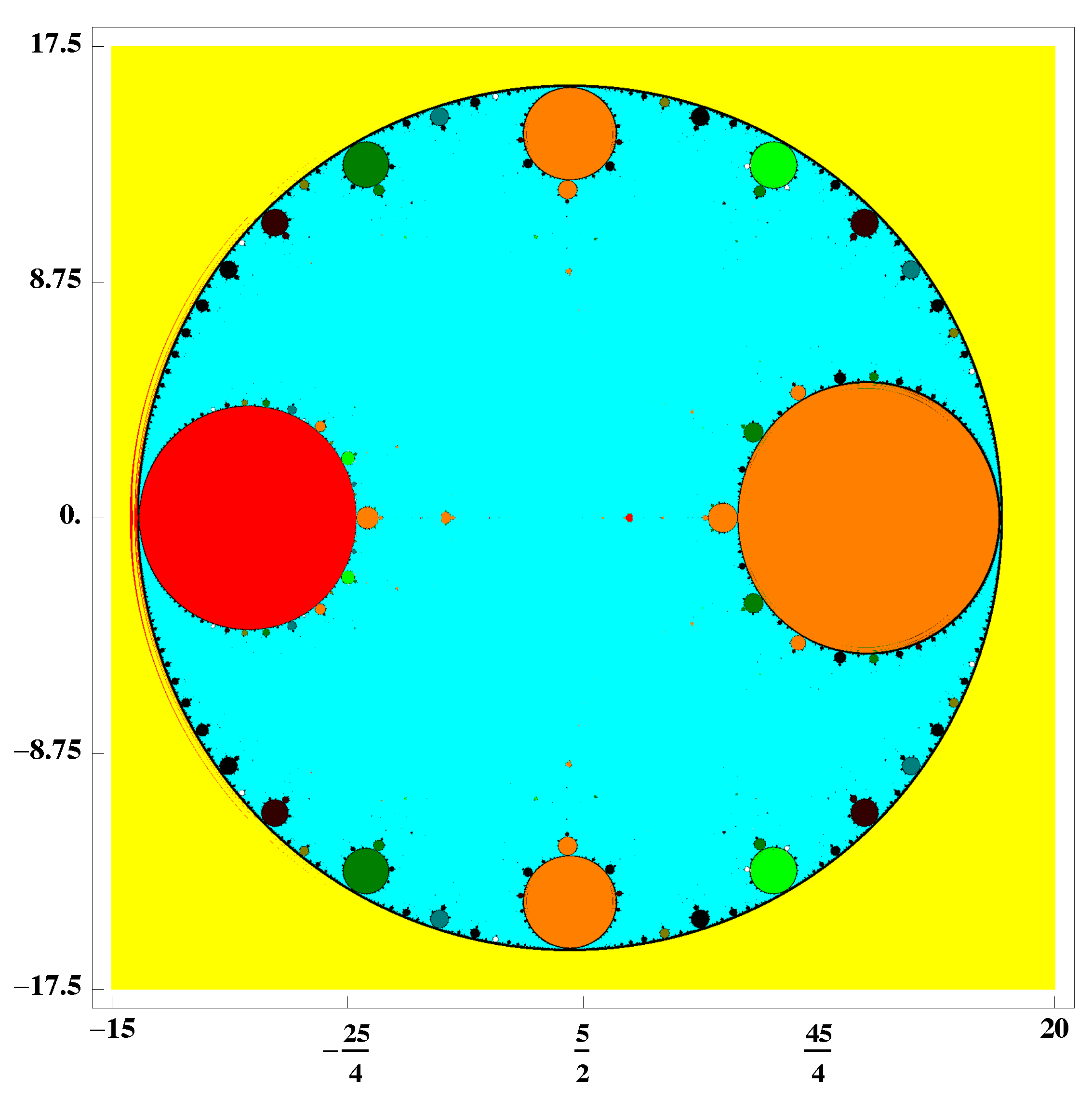
We are going to show different planes of parameters. In Figure 2 we show the parameter spaces associated to critical point c p 2 ( α ) . Now let us paint a point of cyan if the iteration of the method starting in z 0 = c p 1 ( α ) converges to the fixed point 0 (related to root A) or if it converges to (allied to root B). That is, the points relative to the roots of the quadratic polynomial will be painted cyan and a point is painted in yellow if the iteration converges to 1 (related to ). Therefore, all convergence will be painted cyan. On the other hand, convergence to strange fixed points or cycles appears in other colors. As an immediate consequence, all points of the plane that are not cyan are not a good choice of α in terms of numerical behavior.
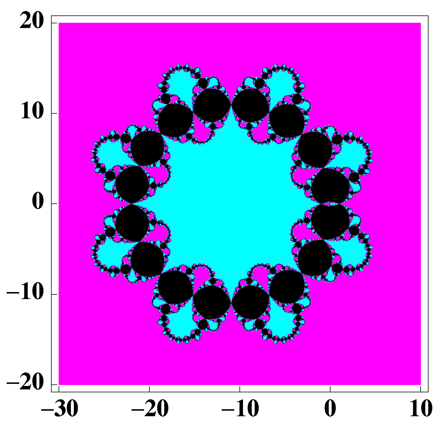
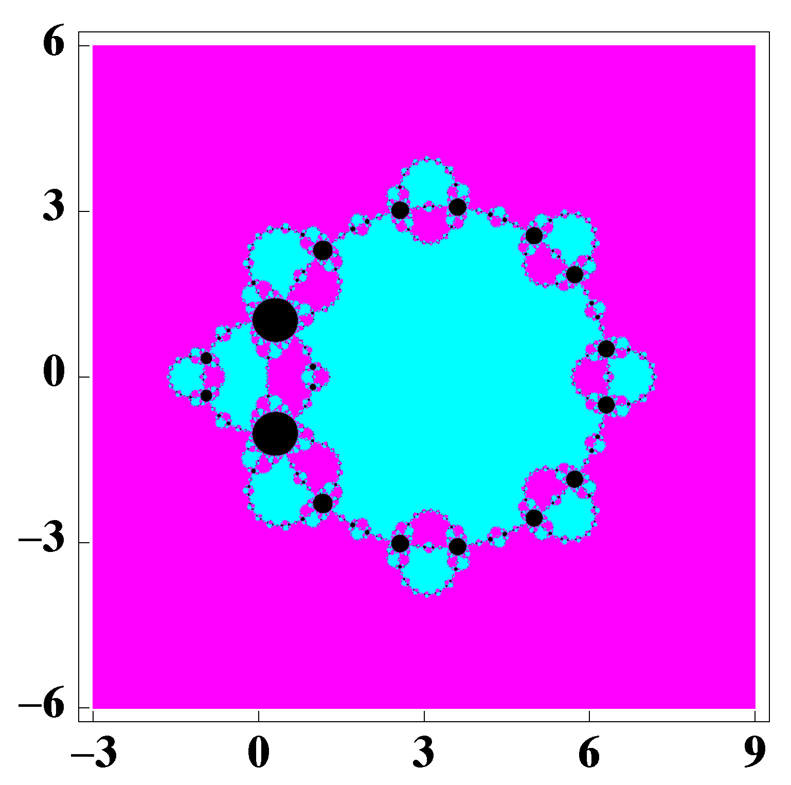
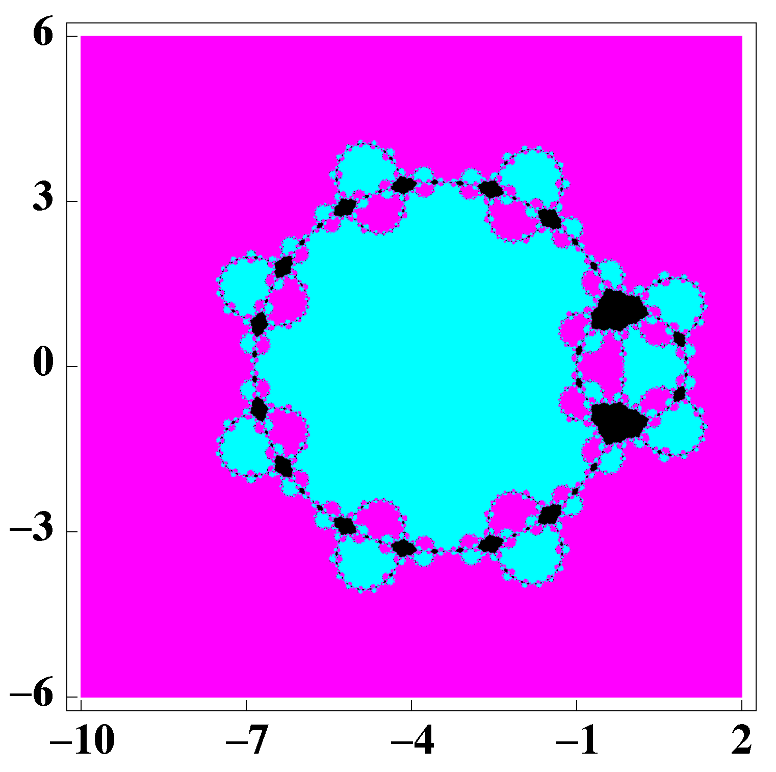
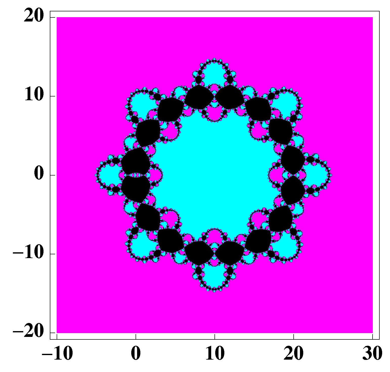
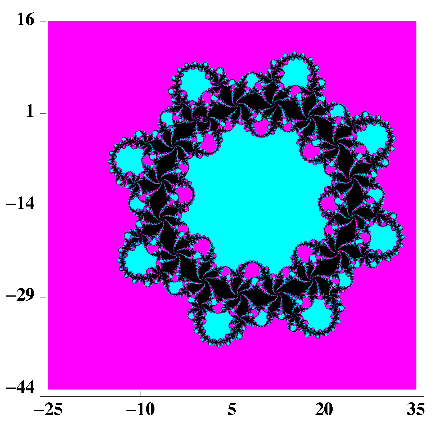
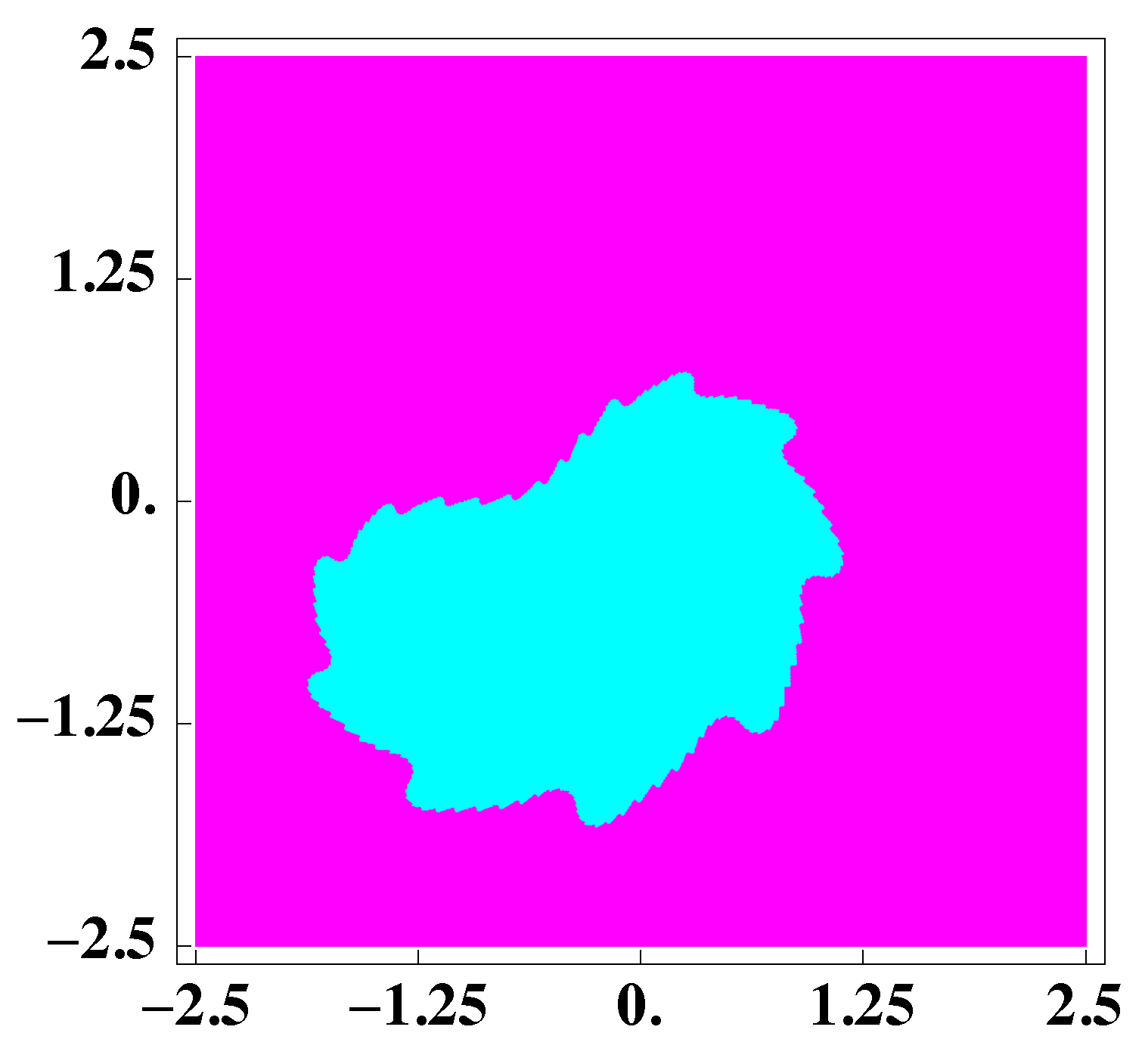
Once we have detected the anomalies, we can go on to describe the dynamic planes. To understand the colors we have used in these dynamic planes, we have to indicate that if after a maximum of 1000 iterations and with a tolerance of 10 6 convergence has not been achieved to the roots, we have painted in black. Conversely, we colored in magenta the convergence to 0 and colored in cyan the convergence to . Then, the cyan or magenta regions identify the convergence.
If we focus our attention on the region shown in Figure 2, it is clear that there are family members with complicated behaviors. We will also show dynamic planes in Figure 3 and Figure 4, of a family member with convergence regions to any of the strange fixed points.
In the following figures, we will show the dynamic planes of family members with convergence to different attracting n-cycles. For example, in the Figure 5 and Figure 6, we see the dynamic planes to an attracting 2-cycle and in the Figure 7 the dynamic plane of family members with convergence to an attracting 3-cycle that was painted in green in the parameter planes.
Other particular cases are shown in Figure 8 and Figure 9. The basins of attraction for different α values in which we see the convergence to the roots of the method can be seen.

4. Example Applied

Next, we want to show the applicability of the theoretical part previously seen in a real problem. Chemistry is a discipline in which many equations are handled. In this concrete case, let us consider the quartic equation that can describe the fraction or amount of the nitrogen-hydrogen feed that is turned into ammonia, which is known as fractional conversion and is shown in [42,43].
If the pressure is 250 atm. and the temperature reaches a value of 500 C, the previous equation reduces to: g ( x ) = x 4 7.79075 x 3 + 14.7445 x 2 + 2.511 x 1.674 . We define S as all real line, D as the interval [ 0 , 1 ] and ξ = 0 . We consider the function F defined on D. If we now take the functions ψ i ( t ) with i = 1 , 2 , 3 and choosing the value of as α = 1.025 , we obtain: L 0 = 2.594 , L = 3.282 . It is clear that in this case L 0 < L , so we improve the results. Now, we compute M = 1.441 . Additionally, computing the zeros of the functions previously defined, we get: r 0 = 0.227 , ϱ A = 0.236 , r 1 = 0.082 , r 2 = 0.155 , r 3 = 0.245 , and as a result of it we get r = r 1 = 0.082 . Then we can guarantee that the method (2) converges for α = 1.025 due to Theorem 1. The applicability of our family of methods is thus proven.

Author Contributions

All authors have contributed equally in writing this article. All authors read and approved the final manuscript.

Funding

This research was funded by Programa de Apoyo a la investigaciń de la fundaciń Séneca-Agencia de Ciencia y Tecnología de la Región de Murcia19374/PI/14’ and by the project MTM2014-52016-C2-1-P of the Spanish Ministry of Science and Innovation.

Conflicts of Interest

The authors declare no conflict of interest.

References

  1. Tello, J.I.C.; Orcos, L.; Granados, J.J.R. Virtual forums as a learning method in Industrial Engineering Organization. IEEE Latin Am. Trans. 2016, 14, 3023–3028. [Google Scholar] [CrossRef]
  2. LeTendre, G.; McGinnis, E.; Mitra, D.; Montgomery, R.; Pendola, A. The American Journal of Education: Challenges and opportunities in translational science and the grey area of academic. Rev. Esp. Pedag. 2018, 76, 413–435. [Google Scholar] [CrossRef]
  3. Argyros, I.K.; González, D. Local convergence for an improved Jarratt–type method in Banach space. Int. J. Interact. Multimed. Artif. Intell. 2015, 3, 20–25. [Google Scholar] [CrossRef]
  4. Argyros, I.K.; George, S. Ball convergence for Steffensen–type fourth-order methods. Int. J. Interact. Multimed. Artif. Intell. 2015, 3, 27–42. [Google Scholar] [CrossRef]
  5. Argyros, I.K.; Magreñán, Á.A. Iterative Methods and Their Dynamics with Applications: A Contemporary Study; CRC-Press: Boca Raton, FL, USA, 2017. [Google Scholar]
  6. Behl, R.; Sarría, Í.; González-Crespo, R.; Magreñán, Á.A. Highly efficient family of iterative methods for solving nonlinear models. J. Comput. Appl. Math. 2019, 346, 110–132. [Google Scholar] [CrossRef]
  7. Magreñán, Á.A.; Argyros, I.K. A Contemporary Study of Iterative Methods: Convergence, Dynamics and Applications; Elsevier: Amsterdam, The Netherlands, 2018. [Google Scholar]
  8. Rheinboldt, W.C. An adaptive continuation process for solving systems of nonlinear equations. Pol. Acad. Sci. 1978, 3, 129–142. [Google Scholar] [CrossRef] [Green Version]
  9. Amat, S.; Busquier, S.; Plaza, S. Dynamics of the King and Jarratt iterations. Aequ. Math. 2005, 69, 212–223. [Google Scholar] [CrossRef]
  10. Amat, S.; Busquier, S.; Plaza, S. Chaotic dynamics of a third-order Newton-type method. J. Math. Anal. Appl. 2010, 366, 24–32. [Google Scholar] [CrossRef] [Green Version]
  11. Amat, S.; Hernández, M.A.; Romero, N. A modified Chebyshev’s iterative method with at least sixth order of convergence. Appl. Math. Comput. 2008, 206, 164–174. [Google Scholar] [CrossRef]
  12. Chicharro, F.; Cordero, A.; Torregrosa, J.R. Drawing dynamical and parameters planes of iterative families and methods. Sci. World J. 2013, 2013, 780153. [Google Scholar] [CrossRef] [PubMed]
  13. Gutiérrez, J.M.; Hernández, M.A. Recurrence relations for the super-Halley method. Comput. Math. Appl. 1998, 36, 1–8. [Google Scholar] [CrossRef] [Green Version]
  14. Kou, J.; Li, Y. An improvement of the Jarratt method. Appl. Math. Comput. 2007, 189, 1816–1821. [Google Scholar] [CrossRef]
  15. Li, D.; Liu, P.; Kou, J. An improvement of the Chebyshev-Halley methods free from second derivative. Appl. Math. Comput. 2014, 235, 221–225. [Google Scholar] [CrossRef]
  16. Magreñán, Á.A. Different anomalies in a Jarratt family of iterative root-finding methods. Appl. Math. Comput. 2014, 233, 29–38. [Google Scholar]
  17. Budzko, D.; Cordero, A.; Torregrosa, J.R. A new family of iterative methods widening areas of convergence. Appl. Math. Comput. 2015, 252, 405–417. [Google Scholar] [CrossRef] [Green Version]
  18. Bruns, D.D.; Bailey, J.E. Nonlinear feedback control for operating a nonisothermal CSTR near an unstable steady state. Chem. Eng. Sci. 1977, 32, 257–264. [Google Scholar] [CrossRef]
  19. Candela, V.; Marquina, A. Recurrence relations for rational cubic methods I: The Halley method. Computing 1990, 44, 169–184. [Google Scholar] [CrossRef]
  20. Candela, V.; Marquina, A. Recurrence relations for rational cubic methods II: The Chebyshev method. Computing 1990, 45, 355–367. [Google Scholar] [CrossRef]
  21. Ezquerro, J.A.; Hernández, M.A. New iterations of R-order four with reduced computational cost. BIT Numer. Math. 2009, 49, 325–342. [Google Scholar] [CrossRef]
  22. Ezquerro, J.A.; Hernández, M.A. On the R-order of the Halley method. J. Math. Anal. Appl. 2005, 303, 591–601. [Google Scholar] [CrossRef] [Green Version]
  23. Ganesh, M.; Joshi, M.C. Numerical solvability of Hammerstein integral equations of mixed type. IMA J. Numer. Anal. 1991, 11, 21–31. [Google Scholar] [CrossRef]
  24. Hernández, M.A. Chebyshev’s approximation algorithms and applications. Comput. Math. Appl. 2001, 41, 433–455. [Google Scholar] [CrossRef]
  25. Hernández, M.A.; Salanova, M.A. Sufficient conditions for semilocal convergence of a fourth order multipoint iterative method for solving equations in Banach spaces. Southwest J. Pure Appl. Math. 1999, 1, 29–40. [Google Scholar]
  26. Jarratt, P. Some fourth order multipoint methods for solving equations. Math. Comput. 1966, 20, 434–437. [Google Scholar] [CrossRef]
  27. Ren, H.; Wu, Q.; Bi, W. New variants of Jarratt method with sixth-order convergence. Numer. Algorithms 2009, 52, 585–603. [Google Scholar] [CrossRef]
  28. Traub, J.F. Iterative Methods for the Solution of Equations; Prentice-Hall Series in Automatic Computation: Englewood Cliffs, NJ, USA, 1964. [Google Scholar]
  29. Wang, X.; Kou, J.; Gu, C. Semilocal convergence of a sixth-order Jarratt method in Banach spaces. Numer. Algorithms 2011, 57, 441–456. [Google Scholar] [CrossRef]
  30. Cordero, A.; Torregrosa, J.R.; Vindel, P. Dynamics of a family of Chebyshev-Halley type methods. Appl. Math. Comput. 2013, 219, 8568–8583. [Google Scholar] [CrossRef]
  31. Artidiello, S.; Cordero, A.; Torregrosa, J.R.; Vassileva, M.P. Optimal high order methods for solving nonlinear equations. J. Appl. Math. 2014, 2014, 591638. [Google Scholar] [CrossRef]
  32. Petković, M.; Neta, B.; Petković, L.; Džunić, J. Multipoint Methods for Solving Nonlinear Equations; Elsevier: Amsterdam, The Netherlands, 2013. [Google Scholar]
  33. Zhao, L.; Wang, X.; Guo, W. New families of eighth-order methods with high efficiency index for solving nonlinear equations. Wseas Trans. Math. 2012, 11, 283–293. [Google Scholar]
  34. Dźunic, J.; Petković, M. A family of Three-Point methods of Ostrowski’s Type for Solving Nonlinear Equations. J. Appl. Math. 2012, 2012, 425867. [Google Scholar] [CrossRef]
  35. Chun, C. Some improvements of Jarratt’s method with sixth-order convergence. Appl. Math. Comput. 1990, 190, 1432–1437. [Google Scholar] [CrossRef]
  36. Cordero, A.; Torregrosa, J.R. Variants of Newton’s method using fifth-order quadrature formulas. Appl. Math. Comput. 2007, 190, 686–698. [Google Scholar] [CrossRef]
  37. Ezquerro, J.A.; Hernández, M.A. Recurrence relations for Chebyshev-type methods. Appl. Math. Optim. 2000, 41, 227–236. [Google Scholar] [CrossRef]
  38. Magreñán, Á.A. A new tool to study real dynamics: The convergence plane. Appl. Math. Comput. 2014, 248, 215–224. [Google Scholar] [CrossRef] [Green Version]
  39. Rall, L.B. Computational Solution of Nonlinear Operator Equations; Robert E. Krieger: New York, NY, USA, 1979. [Google Scholar]
  40. Weerakon, S.; Fernando, T.G.I. A variant of Newton’s method with accelerated third-order convergence. Appl. Math. Lett. 2000, 13, 87–93. [Google Scholar] [CrossRef]
  41. Cordero, A.; García-Maimó, J.; Torregrosa, J.R.; Vassileva, M.P.; Vindel, P. Chaos in King’s iterative family. Appl. Math. Lett. 2013, 26, 842–848. [Google Scholar] [CrossRef] [Green Version]
  42. Gopalan, V.B.; Seader, J.D. Application of interval Newton’s method to chemical engineering problems. Reliab. Comput. 1995, 1, 215–223. [Google Scholar]
  43. Shacham, M. An improved memory method for the solution of a nonlinear equation. Chem. Eng. Sci. 1989, 44, 1495–1501. [Google Scholar] [CrossRef]
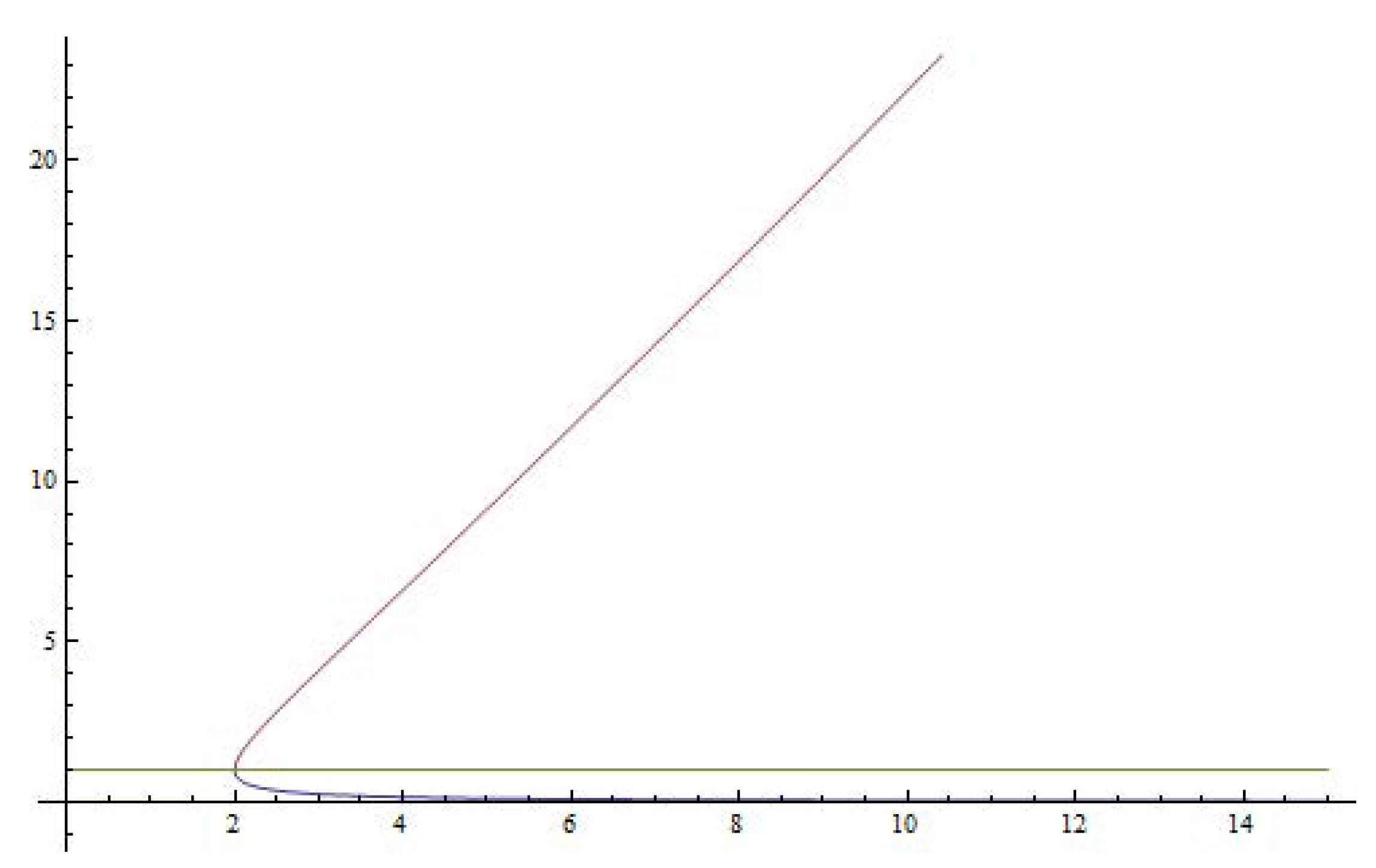
Figure 1. Fixed points’s bifurcation diagram.
Mathematics 07 00225 g001
Figure 2. Parameter space of the free critical point c p 2 ( α ) .
Mathematics 07 00225 g002
Figure 3. Attraction basins associated to α = 10 .
Mathematics 07 00225 g003
Figure 4. Attraction basins associated to α = 4.25 .
Mathematics 07 00225 g004
Figure 5. Attraction basins associated to α = 2.5 .
Mathematics 07 00225 g005
Figure 6. Attraction basins associated to α = 11 .
Mathematics 07 00225 g006
Figure 7. Attraction basins associated to α = 10 13 i .
Mathematics 07 00225 g007
Figure 8. Attraction basins associated to α = 0.5 .
Mathematics 07 00225 g008
Figure 9. Attraction basins associated to α = 0.5 i .
Mathematics 07 00225 g009