Solving Non-Linear Fractional Variational Problems Using Jacobi Polynomials

Abstract

The aim of this paper is to solve a class of non-linear fractional variational problems (NLFVPs) using the Ritz method and to perform a comparative study on the choice of different polynomials in the method. The Ritz method has allowed many researchers to solve different forms of fractional variational problems in recent years. The NLFVP is solved by applying the Ritz method using different orthogonal polynomials. Further, the approximate solution is obtained by solving a system of nonlinear algebraic equations. Error and convergence analysis of the discussed method is also provided. Numerical simulations are performed on illustrative examples to test the accuracy and applicability of the method. For comparison purposes, different polynomials such as 1) Shifted Legendre polynomials, 2) Shifted Chebyshev polynomials of the first kind, 3) Shifted Chebyshev polynomials of the third kind, 4) Shifted Chebyshev polynomials of the fourth kind, and 5) Gegenbauer polynomials are considered to perform the numerical investigations in the test examples. Further, the obtained results are presented in the form of tables and figures. The numerical results are also compared with some known methods from the literature.

1. Introduction

It is necessary to determine the maxima and minima of certain functionals in study problems in analysis, mechanics, and geometry. These problems are known as variational problems in calculus of variations. Variational problems have many applications in various fields like physics [1], engineering [2], and areas in which energy principles are applicable [3,4,5].

Nowadays, fractional calculus is a very interesting branch of mathematics. Fractional calculus has many real applications in science and engineering, such as fluid dynamics [6], biology [7], chemistry [8], viscoelasticity [9,10], signal processing [11], bioengineering [12], control theory [13], and physics [14]. Due to the importance of the fractional derivatives established through real-life applications, several authors have considered problems in calculus of variations by replacing the integer-order derivative with fractional orders in objective functionals, and this is thus known as fractional calculus of variations. Some of these studies are of a fractionally damped system [15], energy control for a fractional linear control system [16], a fractional model of a vibrating string [17], and an optimal control problem [18]. In this paper, our aim is to minimize non-linear fractional variational problems (NLFVPs) [19] of the following form:

$$J\left(y\right)={\int }_0^1{\left(g\left(x\right)D^{\alpha }y\left(x\right)+g^{\prime }\left(x\right)I^{1-\alpha }y\left(x\right)+h^{\prime }\left(x\right)\right)}^{2}dx$$

(1)

under the constraints

$$y\left(0\right)=a,I^{1-\alpha }y\left(1\right)=ϵ,$$

(2)

where $g$ and $h$ are two functions of class $C^1$ with $g\left(x\right)\ne 0$ on $\left[0,1\right]$, $\alpha$ and $ϵ$ are real numbers with $\alpha \in \left(0,1\right)$, and $a$ is a constant.

The pioneer approach for solving the fractional variational problems originates in reference [20] where Agrawal derived the formulation of the Euler-Langrage equation for fractional variational problems. Further, in reference [4], he gave a general formulation for fractional variational problems. In reference [5], the authors used an analytical algorithm based on the Adomian decomposition method (ADM) for solving problems in calculus of variations. In [21,22], Legendre orthonormal polynomials and Jacobi orthonormal polynomials, respectively, were used to obtain an approximate numerical solution of fractional optimum control problems. In [23], the Haar wavelet method was used to obtain numerical solution of these problems. Some other numerical methods for the approximate solution of fractional variational problems are given in [24,25,26,27,28,29,30,31,32,33,34]. Recently, in [19], the authors gave a new class of fractional variational problems and solved this using a decomposition formula based on Jacobi polynomials. The operational matrix methods (see [35,36,37,38,39,40,41]) have been found to be useful for solving problems in fractional calculus.

In present paper, we extend the Rayleigh-Ritz method together with operational matrices of different orthogonal polynomials such as Shifted Legendre polynomials, Shifted Chebyshev polynomials of the first kind, Shifted Chebyshev polynomials of the third kind, Shifted Chebyshev polynomials of the fourth kind, and Gegenbauer polynomials to solve a special class of NLFVPs. The Rayleigh-Ritz methods have been discussed by many researchers in the literature for different kinds of variational problems, i.e., fractional optimal control problems [18,21,22,32,33]; here we cite only few, and many more can be found in the literature. In this method, first we take a finite-dimensional approximation of the unknown function. Further, using an operational matrix of integration and the Rayleigh-Ritz method in the variational problem, we obtain a system of non-linear algebraic equations whose solution gives an approximate solution for the non-linear variational problem. Error analysis of the method for different orthogonal polynomials is given, and convergence of the approximate numerical solution to the exact solution is shown. A comparative study using absolute error and root-mean-square error tables for all five kinds of polynomials is analyzed. Numerical results are discussed in terms of the different values of fractional order involved in the problem and are shown through tables and figures.

2. Basic Preliminaries

The definition of fractional order integration in the Riemann-Liouville sense is defined as follows.

Definition 1.

The Riemann-Liouville fractional order integral operator is given by

$$I^{\alpha }f\left(x\right)=\{\begin{array}{cccc}\frac{1}{\Gamma \left(\mathsf{\alpha }\right)}{\displaystyle \underset{0}{\overset{x}{\int }}}{\left(x-t\right)}^{\alpha -1}f\left(t\right)dt,& & & \alpha >0,x>0,\hfill \\ f\left(x\right),& & & \alpha =0.\hfill \end{array}$$

The analytical form of the shifted Jacobi polynomial of degree $i$ on [0, 1] is given as

$${\Psi }_i\left(x\right)={\displaystyle \sum _{k=0}^i}{\left(-1\right)}^{i-k}\frac{\Gamma \left(i+b+1\right)\Gamma \left(i+k+a+b+1\right)}{\Gamma \left(k+b+1\right)\Gamma \left(i+a+b+1\right)\left(i-k\right)!k!}{x}^k$$

(3)

where $a$ and $b$ are certain constants. Jacobi polynomials are orthogonal in the interval [0, 1] with respect to the weight function $w^{\left(a,b\right)}\left(x\right)={\left(1-x\right)}^a{x}^b$ and have the orthogonality property

$${\int }_0^1{\Psi }_n\left(x\right){\Psi }_m\left(x\right)w^{\left(a,b\right)}\left(x\right)dx=v_n^{a,b}{\delta }_{mn}$$

(4)

where ${\delta }_{mn}$ is the Kronecker delta function and

$$v_n^{a,b}=\frac{\Gamma \left(n+a+1\right)\Gamma \left(n+b+1\right)}{\left(2n+a+b+1\right)n!\Gamma \left(n+a+b+1\right)}.$$

(5)

For certain values of the constants $a$ and $b$, the Jacobi polynomials take the form of some well-known polynomials, defined as follows.

Case 1: Legendre polynomials (S1) For $a=0,b=0$ in Equation (3), we get Legendre polynomials.

$${\Psi }_i\left(x\right)={\displaystyle \sum _{k=0}^i}{\left(-1\right)}^{i-k}\frac{\Gamma \left(i+1\right)\Gamma \left(i+k+1\right)}{\Gamma \left(k+1\right)\Gamma \left(i+1\right)\left(i-k\right)!k!}{x}^k$$

(6)

Case 2: Chebyshev polynomials of the first kind (S2) For $a=\frac{1}{2},b=\frac{1}{2}$ in Equation (3), we get Chebyshev polynomials of the first kind.

$${\Psi }_i\left(x\right)={\displaystyle \sum _{k=0}^i}{\left(-1\right)}^{i-k}\frac{\Gamma \left(i+\frac{3}{2}\right)\Gamma \left(i+k+2\right)}{\Gamma \left(k+\frac{3}{2}\right)\Gamma \left(i+2\right)\left(i-k\right)!k!}{x}^k$$

(7)

Case 3: Chebyshev polynomials of the third kind (S3) For $a=\frac{1}{2},b=-\frac{1}{2}$ in Equation (3), we get Chebyshev polynomials of the third kind.

$${\Psi }_i\left(x\right)={\displaystyle \sum _{k=0}^i}{\left(-1\right)}^{i-k}\frac{\Gamma \left(i+\frac{1}{2}\right)\Gamma \left(i+k+1\right)}{\Gamma \left(k+\frac{1}{2}\right)\Gamma \left(i+1\right)\left(i-k\right)!k!}{x}^k$$

(8)

Case 4: Chebyshev polynomials of the fourth kind (S4) For $a=-\frac{1}{2},b=\frac{1}{2}$ in Equation (3), we get Chebyshev polynomials of the fourth kind.

$${\Psi }_i\left(x\right)={\displaystyle \sum _{k=0}^i}{\left(-1\right)}^{i-k}\frac{\Gamma \left(i+\frac{3}{2}\right)\Gamma \left(i+k+1\right)}{\Gamma \left(k+\frac{3}{2}\right)\Gamma \left(i+1\right)\left(i-k\right)!k!}{x}^k$$

(9)

Case 5: Gegenbauer polynomials (S5) For $a=b=a-\frac{1}{2}$ in Equation (3), we get Gegenbauer polynomials.

$${\Psi }_i\left(x\right)={\displaystyle \sum _{k=0}^i}{\left(-1\right)}^{i-k}\frac{\Gamma \left(i+a+\frac{1}{2}\right)\Gamma \left(i+k+2a\right)}{\Gamma \left(k+a+\frac{1}{2}\right)\Gamma \left(i+2a\right)\left(i-k\right)!k!}{x}^k$$

(10)

A function $f\in L^2\left[0,1\right]$ with $\left|f^{″}\left(t\right)\right|\le K$ can be expanded as

$$f\left(t\right)=\underset{n\to \infty }{\lim }{\displaystyle \sum _{i=0}^n}{c}_i{\Psi }_i\left(t\right),$$

(11)

where $c_i=⟨f\left(t\right),{\Psi }_i\left(t\right)⟩$ and $⟨-,-⟩$ is the usual inner product space.

Equation (11) for finite-dimensional approximation is written as

$$f\cong {\displaystyle \sum _{i=0}^m}{c}_i{\Psi }_i\left(t\right)=C^T{\varphi }_m\left(t\right),$$

(12)

where $C$ and ${\varphi }_m\left(t\right)$ are $\left(m+1\right)\times 1$ matrices given by $C={\left[c_0,c_1,\dots ,c_m\right]}^T$ and ${\varphi }_m\left(t\right)={\left[{\Psi }_0,{\Psi }_1,\dots ,{\Psi }_m\right]}^T$.

Theorem 1.

Let$H$be a Hilbert space and$Z$be a closed subspace of$H$with dim$Z<\infty$; let$\left\{z_1,z_2,\dots ,z_N\right\}$be any basis for$Z$. Suppose that$y$is an arbitrary element in$H$and$z_0$is the unique best approximation to$y$out of$Z$. Then

$${\Vert y-z_0\Vert }_2^2=\frac{T\left(y;z_1,z_2,\dots ,z_N\right)}{T\left(z_1,z_2,\dots ,z_N\right)},$$

where

$$T\left(y;z_1,z_2,\dots ,z_N\right)=\left|\begin{array}{cccc}⟨y,y⟩& ⟨y,Z_1⟩& \cdots & ⟨y,Z_N⟩\\ ⟨Z_1,Z_N⟩& ⟨Z_1,Z_1⟩& \cdots & ⟨Z_1,Z_N⟩\\ ·& ·& ⋮& ·\\ ·& ·& ⋮& ·\\ ·& ·& ⋮& ·\\ ⟨Z_N,y⟩& ⟨Z_N,Z_1⟩& \cdots & ⟨Z_N,Z_N⟩\end{array}\right|.$$

Proof .

Please see references [42,43]. □

Theorem 2.

Suppose that$f_N\left(x\right)$is the Nth approximation of the function$f\in L_{w^{\left(a,b\right)}}^2\left[0,1\right]$, and suppose

$$S_N\left(f\right)={\int }_0^1{\left[f\left(x\right)-f_N\left(x\right)\right]}^2{w}^{\left(a,b\right)}\left(x\right)dx;$$

then we have

$$\underset{N\to \infty }{\lim }{S}_N\left(f\right)=0.$$

Proof .

Please see Appendix A. □

3. Operational Matrices

Theorem 3.

Let${\varphi }_n={\left[{\Psi }_0\left(x\right),{\Psi }_1\left(x\right),\dots ,{\Psi }_n\left(x\right)\right]}^T$be a Shifted Jacobi vector and suppose$v>0$; then

$$I^v{\Psi }_i\left(x\right)=I^{\left(v\right)}{\varphi }_n\left(x\right)$$

where$I^{\left(v\right)}=\left(\mu \left(i,j\right)\right)$is an$\left(n+1\right)\times \left(n+1\right)$operational matrix of the fractional integral of order$v$and its$\left(i,j\right)$th entry is given by

$$\mu \left(i,j\right)={\displaystyle \sum _{k=0}^i\sum _{l=0}^j}{\left(-1\right)}^{i+j-k-l}\frac{\Gamma \left(a+1\right)\Gamma \left(i+b+1\right)\Gamma \left(i+k+a+b+1\right)\Gamma \left(j+l+a+b+1\right)\Gamma \left(v+k+l+a+b+1\right)\left(2j+a+b+1\right)j!}{\left(i-k\right)!\left(j-l\right)!\left(l\right)!\Gamma \left(k+b+1\right)\Gamma \left(i+a+b+1\right)\Gamma \left(v+k+1\right)\Gamma \left(j+a+1\right)\Gamma \left(l+b+1\right)\Gamma \left(k+l+v+a+b+1\right)}.$$

(13)

Proof .

We refer to reference [44] for the proof. □

Now, in particular cases, the operational matrix of integration for various polynomials is given as follows.

For Shifted Legendre polynomials (S1), the $\left(i,j\right)$th entry of the operational matrix of integration is given as

$$\mu \left(i,j\right)={\displaystyle \sum _{k=0}^i\sum _{l=0}^j}{\left(-1\right)}^{i+j+k+l}\frac{\left(i+k\right)!\left(j+l\right)!}{\left(i-k\right)!\left(j-l\right)!\left(k\right)!{\left(l!\right)}^2\left(\alpha +k+l+1\right)\Gamma \left(\alpha +k+l\right)}.$$

(14)

For Shifted Chebyshev polynomials of the first kind (S2), the $\left(i,j\right)$th entry of the operational matrix of integration is given as:

$$\mu \left(i,j\right)={\displaystyle \sum _{k=0}^i\sum _{l=0}^j}{\left(-1\right)}^{i+j-k-l}\frac{\Gamma \left(\frac{3}{2}\right)\Gamma \left(i+\frac{3}{2}\right)\Gamma \left(i+k+2\right)\Gamma \left(j+l+2\right)\Gamma \left(\alpha +k+l+\frac{3}{2}\right)\left(2j+2\right)j!}{\left(i-k\right)!\left(j-l\right)!\left(l\right)!\Gamma \left(k+\frac{3}{2}\right)\Gamma \left(i+2\right)\Gamma \left(\alpha +k+1\right)\Gamma \left(j+\frac{3}{2}\right)\Gamma \left(l+\frac{3}{2}\right)\Gamma \left(k+l+\alpha +3\right)}.$$

(15)

For Shifted Chebyshev polynomials of the third kind (S3), the $\left(i,j\right)$th entry of the operational matrix of integration is given as

$$\mu \left(i,j\right)={\displaystyle \sum _{k=0}^i\sum _{l=0}^j}{\left(-1\right)}^{i+j-k-l}\frac{\Gamma \left(\frac{3}{2}\right)\Gamma \left(i+\frac{1}{2}\right)\Gamma \left(i+k+1\right)\Gamma \left(j+l+1\right)\Gamma \left(\alpha +k+l+\frac{1}{2}\right)\left(2j+1\right)j!}{\left(i-k\right)!\left(j-l\right)!\left(l\right)!\Gamma \left(k+\frac{1}{2}\right)\Gamma \left(i+1\right)\Gamma \left(\alpha +k+1\right)\Gamma \left(j+\frac{3}{2}\right)\Gamma \left(l+\frac{1}{2}\right)\Gamma \left(k+l+\alpha +2\right)}.$$

(16)

For Shifted Chebyshev polynomials of the fourth kind (S4), the $\left(i,j\right)$th entry of the operational matrix of integration is given as

$$\mu \left(i,j\right)={\displaystyle \sum _{k=0}^i\sum _{l=0}^j}{\left(-1\right)}^{i+j-k-l}\frac{\Gamma \left(\frac{1}{2}\right)\Gamma \left(i+\frac{3}{2}\right)\Gamma \left(i+k+1\right)\Gamma \left(j+l+1\right)\Gamma \left(\alpha +k+l+\frac{3}{2}\right)\left(2j+1\right)j!}{\left(i-k\right)!\left(j-l\right)!\left(l\right)!\Gamma \left(k+\frac{3}{2}\right)\Gamma \left(i+1\right)\Gamma \left(\alpha +k+1\right)\Gamma \left(j+\frac{1}{2}\right)\Gamma \left(l+\frac{3}{2}\right)\Gamma \left(k+l+\alpha +2\right)}.$$

(17)

For Shifted Gegenbauer polynomials (S5), the $\left(i,j\right)$th entry of the operational matrix of integration is given as

$$\mu \left(i,j\right)={\displaystyle \sum _{k=0}^i\sum _{l=0}^j}{\left(-1\right)}^{i+j-k-l}\frac{\Gamma \left(i+a+\frac{1}{2}\right)\Gamma \left(i+k+2a\right)\Gamma \left(j+l+2a\right)\Gamma \left(a+\frac{1}{2}\right)\Gamma \left(\alpha +k+l+a+\frac{1}{2}\right)\left(2j+2a\right)j!}{\left(i-k\right)!\left(j-l\right)!\left(l\right)!\Gamma \left(k+a+\frac{1}{2}\right)\Gamma \left(i+2a\right)\Gamma \left(\alpha +k+1\right)\Gamma \left(j+a+\frac{1}{2}\right)\Gamma \left(l+a+\frac{1}{2}\right)\Gamma \left(2a+k+l+\alpha +1\right)}.$$

(18)

4. Method of Solution

Approximating the unknown function in terms of orthogonal polynomials has been practiced in several papers in recent years [18,21,22,32,33] for different types of problems. Here, for solving the problem in Equation (1), we approximate

$$D^{\alpha }y\left(x\right)=C^T{\Phi }_n\left(x\right).$$

(19)

We are approximating the derivative first because we want to use the initial condition. Taking the integral of order $\alpha$ on both sides of Equation (19), we get

$$y\left(x\right)=C^T{I}^{\alpha }{\Phi }_n\left(x\right)+y\left(0\right).$$

(20)

Using the operational matrix of integration, Equation (20) can be written as

$$y\left(x\right)\cong C^T{I}^{\left(\alpha \right)}{\Phi }_n\left(x\right)+A^T{\Phi }_n\left(x\right)$$

(21)

where $y\left(0\right)=a\cong A^T{\Phi }_n\left(x\right)$ and $I^{\left(\alpha \right)}$ is the operational matrix of integration of order $\alpha$.

Using Equation (19), we can write

$$I^{1-\alpha }y\left(x\right)=I{D}^{\alpha }y\left(x\right)=C^{T}I{\Phi }_n\left(x\right)\cong C^T{I}^{\left(1\right)}{\Phi }_n\left(x\right).$$

(22)

Using Equations (19) and (22) in Equation (1), we obtain

$$J\left(c_0,c_1,\dots ,c_n\right)={\int }_0^1{\left(g\left(x\right)C^T{\Phi }_n\left(x\right)+g^{\prime }\left(x\right)C^{T}I{\Phi }_n\left(x\right)+h^{\prime }\left(x\right)\right)}^{2}dx.$$

(23)

Equation (23) can then be written as

$$J\left(c_0,c_1,\dots ,c_n\right)={\int }_0^1{\left(C^{T}g\left(x\right){\Phi }_n\left(x\right)+C^T{I}^{\left(1\right)}{g}^{\prime }\left(x\right){\Phi }_n\left(x\right)+h^{\prime }\left(x\right)\right)}^{2}dx.$$

(24)

We further take the following approximations:

$$g\left(x\right){\Phi }_i\left(x\right)\cong E_1^{i,T}{\Phi }_n\left(x\right)$$

(25)

$$g^{\prime }\left(x\right){\Phi }_i\left(x\right)\cong E_2^{i,T}{\Phi }_n\left(x\right)$$

(26)

$$h^{\prime }\left(x\right)\cong E_3^T{\Phi }_n\left(x\right)$$

(27)

where $E_1^{i,T}=[e_{1,0}^i,e_{1,1}^i,\dots ,e_{1,n}^i]$, $E_2^{i,T}=[e_{2,0}^i,e_{2,1}^i,\dots ,e_{2,n}^i]$, $E_3^T=[e_{3,0},e_{3,1},\dots ,e_{3,n}]$, and $e_{1,j}^i=⟨g(x){\Phi }_i(x),{\Psi }_j(x)⟩$, $e_{2,j}^i=⟨g^{\prime }(x){\Phi }_i(x),{\Psi }_j(x)⟩$, $e_{3,j}=⟨h^{\prime }(x),{\Psi }_j(x)⟩$, $0\le i,j\le n$, and $⟨-,-⟩$ is the usual inner product space.

Using Equations (25) and (26) we can write

$$g\left(x\right){\Phi }_n\left(x\right)\cong E_1^T{\Phi }_n\left(x\right)$$

(28)

$$g^{\prime }\left(x\right){\Phi }_n\left(x\right)\cong E_2^T{\Phi }_n\left(x\right)$$

(29)

where

$$E_1^T={\left(E_1^{i,T}\right)}_{0\le i\le n}\mathrm{and}{E}_2^T={\left(E_2^{i,T}\right)}_{0\le i\le n}.$$

(30)

From Equations (24) and (27)–(29), we get

$$J\left(c_0,c_1,\dots ,c_n\right)={\int }_0^1{\left(C^T{E}_1^T{\Phi }_n\left(x\right)+C^T{I}^{\left(1\right)}{E}_2^T{\Phi }_n\left(x\right)+E_3^T{\Phi }_n\left(x\right)\right)}^{2}dx.$$

(31)

Let

$$E^T=C^T\left(E_1^T+I^{\left(1\right)}{E}_2^T\right)+E_3^T.$$

(32)

From Equations (31) and (32), we get

$$\begin{array}{cc}J\left(c_0,c_1,\dots ,c_n\right)& ={\int }_0^1{\left(E^T{\Phi }_n\left(x\right)\right)}^{2}dx\hfill \\ & ={\int }_0^1{E}^T{\Phi }_n\left(x\right){\Phi }_n{\left(x\right)}^{T}E\mathrm{d}x,\hfill \\ & =E^{T}PE\hfill \end{array}$$

(33)

where $P$ is a square matrix given by $P={\int }_0^1{\Phi }_n\left(x\right){\Phi }_n{\left(x\right)}^{T}dx$.

Using Equation (22), the boundary condition can be written as

$$I^{1-\alpha }y\left(1\right)\cong C^T{I}^{\left(1\right)}{\Phi }_n\left(1\right)=ϵ.$$

(34)

Using the Lagrange multiplier method [18,20,21,22,32,33], the necessary extremal condition for the functional in Equation (33) becomes

$$\frac{\partial J}{\partial c_0}=0,\frac{\partial J}{\partial c_1}=0,\dots ,\frac{\partial J}{\partial c_{n-1}}=0.$$

(35)

From Equations (34) and (35), we get a set of $n+1$ equations. Solving these $n+1$ equations, we get unknown parameters $c_0,c_1,\dots ,c_n$. Using these unknown parameters in Equation (21), we get the unknown function’s extreme values of the non-linear fractional functional.

5. Error Analysis

The upper bound of error for the operational matrix of fractional integration of a Jacobi polynomial of the ith degree is given as

$$e_i^{\alpha }=I^{\left(\alpha \right)}{\Psi }_i\left(x\right)-I^{\alpha }{\Psi }_i\left(x\right).$$

(36)

From Equation (36), we can write

$${\Vert e_i^{\alpha }\Vert }_2=\Vert I^{\alpha }{\Psi }_i\left(x\right)-{\displaystyle \sum _{j=0}^n}\mu \left(i,j\right){\Psi }_j\left(x\right){\Vert }_2.$$

(37)

Taking the integral operator of order $\alpha$ on both sides of Equation (3), we get

$$I^{\alpha }{\Psi }_i\left(x\right)={\displaystyle \sum _{k=0}^i}{\left(-1\right)}^{i-k}\frac{\Gamma \left(i+b+1\right)\Gamma \left(i+k+a+b+1\right)}{\left(i-k\right)!\Gamma \left(k+b+1\right)\Gamma \left(i+a+b+1\right)\Gamma \left(\alpha +k+1\right)}{x}^{\alpha +k}.$$

(38)

From the construction of the operational matrix we can write

$$\mu \left(i,j\right)={\displaystyle \sum _{k=0}^i}{\left(-1\right)}^{i-k}\frac{\Gamma \left(i+b+1\right)\Gamma \left(i+k+a+b+1\right)}{\left(i-k\right)!\Gamma \left(k+b+1\right)\Gamma \left(i+a+b+1\right)\Gamma \left(\alpha +k+1\right)}{c}_{j,k},j=0,1,\dots ,n.$$

(39)

Using Theorem 1 we can write

$$\Vert x^{\alpha +k}-{\displaystyle \sum _{j=0}^n}{c}_{j,k}{\Psi }_j\left(x\right){\Vert }_2={\left(\frac{T\left(x^{\alpha +k};{\Psi }_0\left(x\right),{\Psi }_1\left(x\right),\dots ,{\Psi }_n\left(x\right)\right)}{T\left({\Psi }_0\left(x\right),{\Psi }_1\left(x\right),\dots ,{\Psi }_n\left(x\right)\right)}\right)}^2.$$

(40)

From Equations (37)–(39), we get

$$\begin{array}{cc}\hfill {\Vert e_i^{\alpha }\Vert }_2=& {\Vert \begin{array}{c}{\displaystyle \sum _{k=0}^i}{\left(-1\right)}^{i-k}\frac{\Gamma \left(i+b+1\right)\Gamma \left(i+k+a+b+1\right)}{\left(i-k\right)!\Gamma \left(k+b+1\right)\Gamma \left(i+a+b+1\right)\Gamma \left(\alpha +k+1\right)}{x}^{\alpha +k}\\ -{\displaystyle \sum _{j=0}^n\sum _{k=0}^i}{\left(-1\right)}^{i-k}\frac{\Gamma \left(i+b+1\right)\Gamma \left(i+k+a+b+1\right)}{\left(i-k\right)!\Gamma \left(k+b+1\right)\Gamma \left(i+a+b+1\right)\Gamma \left(\alpha +k+1\right)}{c}_{j,k}{\Psi }_j\left(x\right)\end{array}\Vert }_2\hfill \\ & \le {\displaystyle \sum _{k=0}^i}\left|\frac{\Gamma \left(i+b+1\right)\Gamma \left(i+k+a+b+1\right)}{\left(i-k\right)!\Gamma \left(k+b+1\right)\Gamma \left(i+a+b+1\right)\Gamma \left(\alpha +k+1\right)}\right|{\Vert x^{\alpha +k}-{\displaystyle \sum _{j=0}^n}{c}_{j,k}{\Psi }_j\left(x\right)\Vert }_2.\hfill \end{array}$$

(41)

Using Equation (40) in Equation (41), we obtain the error bound for the operational matrix of integration of an ith-degree polynomial, which is given as

$$\Vert e_i^{\alpha }{\Vert }_2\le {\displaystyle \sum _{k=0}^i}\left|\frac{\Gamma \left(i+b+1\right)\Gamma \left(i+k+a+b+1\right)}{\left(i-k\right)!\Gamma \left(k+b+1\right)\Gamma \left(i+a+b+1\right)\Gamma \left(\alpha +k+1\right)}\right|{\left(\frac{T\left(x^{\alpha +k};{\Psi }_0\left(x\right),{\Psi }_1\left(x\right),\dots ,{\Psi }_n\left(x\right)\right)}{T\left({\Psi }_0\left(x\right),{\Psi }_1\left(x\right),\dots ,{\Psi }_n\left(x\right)\right)}\right)}^2,i=0,1,2,\dots ,n.$$

(42)

Now, in particular cases, the error bounds for different orthogonal polynomials are given as follows.

Case 1: For Legendre polynomials (S1) the error bound is given as

$$\Vert e_i^{\alpha }{\Vert }_2\le {\displaystyle \sum _{k=0}^i}\left|\frac{\Gamma \left(i+1\right)\Gamma \left(i+k+1\right)}{\left(i-k\right)!\Gamma \left(k+1\right)\Gamma \left(i+1\right)\Gamma \left(\alpha +k+1\right)}\right|{\left(\frac{T\left(x^{\alpha +k};{\Psi }_0\left(x\right),{\Psi }_1\left(x\right),\dots ,{\Psi }_n\left(x\right)\right)}{T\left({\Psi }_0\left(x\right),{\Psi }_1\left(x\right),\dots ,{\Psi }_n\left(x\right)\right)}\right)}^2,i=0,1,2,\dots ,n.$$

(43)

Case 2: For Chebyshev polynomials of the first kind (S2) the error bound is given as

$$\Vert e_i^{\alpha }{\Vert }_2\le {\displaystyle \sum _{k=0}^i}\left|\frac{\Gamma \left(i+\frac{3}{2}\right)\Gamma \left(i+k+2\right)}{\left(i-k\right)!\Gamma \left(k+\frac{3}{2}\right)\Gamma \left(i+2\right)\Gamma \left(\alpha +k+1\right)}\right|{\left(\frac{T\left(x^{\alpha +k};{\Psi }_0\left(x\right),{\Psi }_1\left(x\right),\dots ,{\Psi }_n\left(x\right)\right)}{T\left({\Psi }_0\left(x\right),{\Psi }_1\left(x\right),\dots ,{\Psi }_n\left(x\right)\right)}\right)}^2,i=0,1,2,\dots ,n.$$

(44)

Case 3: For Chebyshev polynomials of the third kind (S3) the error bound is given as

$$\Vert e_i^{\alpha }{\Vert }_2\le {\displaystyle \sum _{k=0}^i}\left|\frac{\Gamma \left(i+\frac{1}{2}\right)\Gamma \left(i+k+1\right)}{\left(i-k\right)!\Gamma \left(k+\frac{1}{2}\right)\Gamma \left(i+1\right)\Gamma \left(\alpha +k+1\right)}\right|{\left(\frac{T\left(x^{\alpha +k};{\Psi }_0\left(x\right),{\Psi }_1\left(x\right),\dots ,{\Psi }_n\left(x\right)\right)}{T\left({\Psi }_0\left(x\right),{\Psi }_1\left(x\right),\dots ,{\Psi }_n\left(x\right)\right)}\right)}^2,i=0,1,2,\dots ,n.$$

(45)

Case 4: For Chebyshev polynomials (S4) the error bound is given as

$$\Vert e_i^{\alpha }{\Vert }_2\le {\displaystyle \sum _{k=0}^i}\left|\frac{\Gamma \left(i+\frac{3}{2}\right)\Gamma \left(i+k1\right)}{\left(i-k\right)!\Gamma \left(k+\frac{3}{2}\right)\Gamma \left(i+1\right)\Gamma \left(\alpha +k+1\right)}\right|{\left(\frac{T\left(x^{\alpha +k};{\Psi }_0\left(x\right),{\Psi }_1\left(x\right),\dots ,{\Psi }_n\left(x\right)\right)}{T\left({\Psi }_0\left(x\right),{\Psi }_1\left(x\right),\dots ,{\Psi }_n\left(x\right)\right)}\right)}^2,i=0,1,2,\dots ,n.$$

(46)

Case 5: For Gegenbauer polynomials (S5) the error bound is given as

$$\Vert e_i^{\alpha }{\Vert }_2\le {\displaystyle \sum _{k=0}^i}\left|\frac{\Gamma \left(i+2\right)\Gamma \left(i+k+3\right)}{\left(i-k\right)!\Gamma \left(k+2\right)\Gamma \left(i+3\right)\Gamma \left(\alpha +k+1\right)}\right|{\left(\frac{T\left(x^{\alpha +k};{\Psi }_0\left(x\right),{\Psi }_1\left(x\right),\dots ,{\Psi }_n\left(x\right)\right)}{T\left({\Psi }_0\left(x\right),{\Psi }_1\left(x\right),\dots ,{\Psi }_n\left(x\right)\right)}\right)}^2,i=0,1,2,\dots ,n.$$

(47)

Let $e_{I,n}^{\alpha ,w}$ denote the error vector for the operational matrix of integration of order $\alpha$ obtained by using $\left(n+1\right)$ orthogonal polynomials in $L_w^2\left[0,1\right]$; then

$$e_{I,n}^{\alpha ,w}=I^{\left(\alpha \right)}{\Phi }_n\left(x\right)-I^{\alpha }{\Phi }_n\left(x\right).$$

(48)

From Theorems 1 and 2 and from Equations (43)–(47), it is clear that as $n\to \infty$ the error vector in Equation (48) tends to zero.

6. Convergence Analysis

A set of orthogonal polynomials on [0, 1] forms a basis for $L_w^2\left[0,1\right]$. Let $S_n$ be the n-dimensional subspace of $L_w^2\left[0,1\right]$ generated by ${\left({\Phi }_i\right)}_{0\le i\le n}$. Thus, every functional on $S_n$ can be written as a linear combination of orthogonal polynomials ${\left({\Phi }_i\right)}_{0\le i\le n}$. The scalars in the linear combinations can be chosen in such a way that the functional minimizes. Let the minimum value of a functional on space $S_n$ be denoted by $m_n$. From the construction of $S_n$ and $m_n$, it is clear that $S_n\subset S_{n+1}$ and $m_{n+1}\ge m_n$.

Theorem 4.

Consider the functional$J$, then

$$\underset{n\to \infty }{\lim }{m}_n=m=\underset{xϵL_w^2\left[0,1\right]}{\underbrace{inf}}J\left[x\right].$$

Proof .

Using Equation (48) in Equation (23), we have

$$J\left(c_0,c_1,\dots ,c_n\right)={\int }_0^1{\left(C^{T}g\left(x\right){\Phi }_n\left(x\right)+C^T{I}^{\left(1\right)}{g}^{\prime }\left(x\right){\Phi }_n\left(x\right)+C^T{e}_{I,n}^1{g}^{\prime }\left(x\right)+h^{\prime }\left(x\right)\right)}^{2}dx.$$

(49)

Taking $n\to \infty$ and using Equations (25)–(27) and (48) in Equation (49), we get

$$\begin{array}{cc}\hfill J^e\left(c_0,c_1,\dots ,c_n\right)& ={\int }_0^1\left(C^T\right({\displaystyle \sum _{i=0}^n}(E_1^{i,T}{\Phi }_n\left(x\right)+e_{E_1^i,n}^w))\hfill \\ & +C^T{I}^{\left(1\right)}{\left({\displaystyle \sum _{i=0}^n}(E_2^{i,T}{\Phi }_n(x)+e_{E_2^i,n}^w))+E_3^T{\Phi }_n\left(x\right)+e_{E_3,n}^w\right)}^{2}dx\hfill \end{array}$$

(50)

where

$$\begin{array}{c}{e}_{E_1^i,n}^w=E_1^{i,T}\Phi \left(x\right)-E_1^{i,T}{\Phi }_n\left(x\right),\\ e_{E_2^i,n}^w=E_2^{i,T}\Phi \left(x\right)-E_2^{i,T}{\Phi }_n\left(x\right),\\ e_{E_3,n}^w=E_3^T\Phi \left(x\right)-E_3^T{\Phi }_n\left(x\right),\end{array}$$

and $J^e$ is the error term of the functional.

Using Equations (30) and (32) in Equation (50), we get

$$J^e\left(c_0,c_1,\dots ,c_n\right)={\int }_0^1{\left(E^T{\Phi }_n\left(x\right)+e_n^w\right)}^{2}dx$$

(51)

where

$$e_n^w=C^T{\displaystyle \sum _{i=0}^n}{e}_{E_1^i,n}^w+C^T{I}^{\left(1\right)}{\displaystyle \sum _{i=0}^n}{e}_{E_2^i,n}^w.$$

(52)

Solving Equation (51) similarly to the original functional, Equation (51) reduces to the following form:

$$J^e\left(c_0,c_1,\dots ,c_n\right)=E^{T}PE+e_n^w\left(J^e\right).$$

(53)

Using Equation (48) in Equation (34), we get

$$C^T{I}^{\left(1\right)}{\Phi }_n\left(1\right)+C^T{e}_{I,n}^{1,w}=ϵ.$$

(54)

Similar to above, by using the Rayleigh-Ritz method on Equation (53) with the boundary condition in Equation (54) we obtain the extreme value of the functional defined in Equation (53). Let this extreme value be denoted by $m_n^{*}\left(t\right)$.

Now, from Equation (48), it is obvious that $e_{E_1^i,n}^w,e_{E_2^i,n}^w,e_{E_3,n}^w\to 0$ as $n\to \infty ,$ which implies that $e_n^w\left(J^e\right)\to 0\mathrm{as}n\to \infty .$ So, it is clear that as $n\to \infty$, the functional $J^e$ in Equation (53) comes close to the functional $J$ in Equation (23) and the boundary condition in Equation (54) comes close to Equation (34).

So, for large values of $n,$

$$m_n^{*}\left(t\right)\to m_n\left(t\right).$$

(55)

From Theorem 4 and Equation (55), we conclude that

$$\underset{n\to \infty }{\lim }{m}_n^{*}\left(t\right)=m\left(t\right).$$

Proof completed. □

7. Numerical Results and Discussions

In this section, we investigate the accuracy of the method by testing it on some numerical examples. We apply the numerical algorithm to two test problems using different orthogonal polynomials as a basis. The results for the test problems are shown through the figures and tables.

Example 1.

Consider a non-linear fractional variational problem as in Equation (1) with$g\left(x\right)=h\left(x\right)=\frac{1}{1+x^{\beta }}$; we then have the following non-linear fractional variational problem [19]:

$$J\left(y\right)={\int }_0^1{\left(\frac{1}{1+x^{\beta }}{D}^{\alpha }y\left(x\right)-\left(I^{1-\alpha }y\left(x\right)+1\right)\frac{\beta x^{\beta -1}}{{\left(1+x^{\beta }\right)}^2}\right)}^{2}dx$$

(56)

under the constraints

$$y\left(0\right)=0,I^{1-\alpha }y\left(1\right)=ϵ.$$

The exact solution of the above equation is given as

$$y_{exact}\left(x\right)=\left(\frac{1}{2}\left(1+ϵ\right)-1\right)\left(\frac{\Gamma \left(\mathsf{\beta }+2\right)}{\Gamma \left(\mathsf{\beta }+\mathsf{\alpha }+1\right)}{x}^{\beta +\alpha }+\frac{1}{\Gamma \left(\mathsf{\alpha }+1\right)}{x}^{\alpha }\right)+\frac{\Gamma \left(\mathsf{\beta }+1\right)}{\Gamma \left(\mathsf{\alpha }+\mathsf{\beta }\right)}{x}^{\beta +\alpha -1}.$$

We discuss this example for different values of $\alpha =0.5,0.6,0.7,0.8,0.9,$ or 1, $\beta =5$, and $ϵ=1.$

In Figure 1, Figure 2, Figure 3, Figure 4 and Figure 5, it is shown that the solutions for the two different values of $\alpha =0.8\mathrm{and}\alpha =1$ coincide with the exact solutions for different orthogonal polynomials at n = 5.

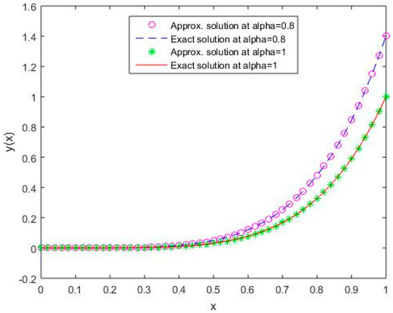
Figure 1. Comparison of exact and numerical solutions using S1 for $\alpha =0.8\mathrm{and}\alpha =1$, Example 1.

Figure 2. Comparison of exact and numerical solutions using S2 for $\alpha =0.8\mathrm{and}\alpha =1$, Example 1.

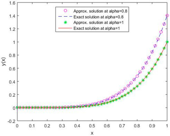
Figure 3. Comparison of exact and numerical solutions using S3 for $\alpha =0.8\mathrm{and}\alpha =1$, Example 1.

Figure 4. Comparison of exact and numerical solutions using S4 for $\alpha =0.8\mathrm{and}\alpha =1$, Example 1.

Figure 5. Comparison of exact and numerical solutions using S5 for $\alpha =0.8\mathrm{and}\alpha =1$, Example 1.

In Figure 6, Figure 7, Figure 8, Figure 9 and Figure 10, it is shown that the solution varies continuously for Shifted Legendre polynomials, Shifted Chebyshev polynomials of the second kind, Shifted Chebyshev polynomials of the third kind, Shifted Chebyshev polynomials of the fourth kind, and Gegenbauer polynomials, respectively, with different values of fractional order.

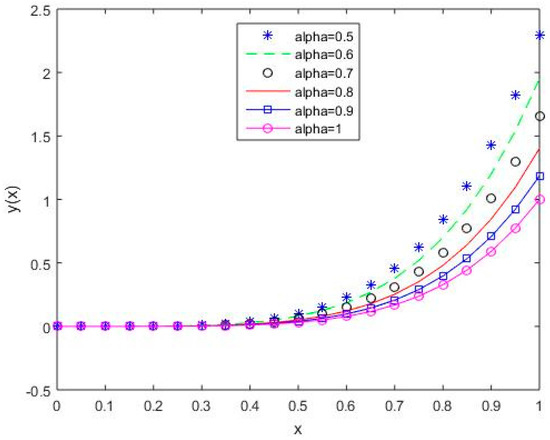
Figure 6. The behavior of solutions using S1 for $\alpha$ values of 0.5, 0.6, 0.7, 0.8, 0.9, and 1, Example 1.

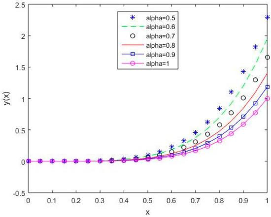
Figure 7. The behavior of solutions using S2 for $\alpha$ values of 0.5, 0.6, 0.7, 0.8, 0.9, and 1, Example 1.

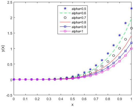
Figure 8. The behavior of solutions using S3 for $\alpha$ values of 0.5, 0.6, 0.7, 0.8, 0.9, and 1, Example 1.

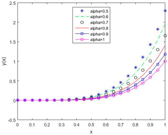
Figure 9. The behavior of solutions using S4 for $\alpha$ values of 0.5, 0.6, 0.7, 0.8, 0.9, and 1, Example 1.

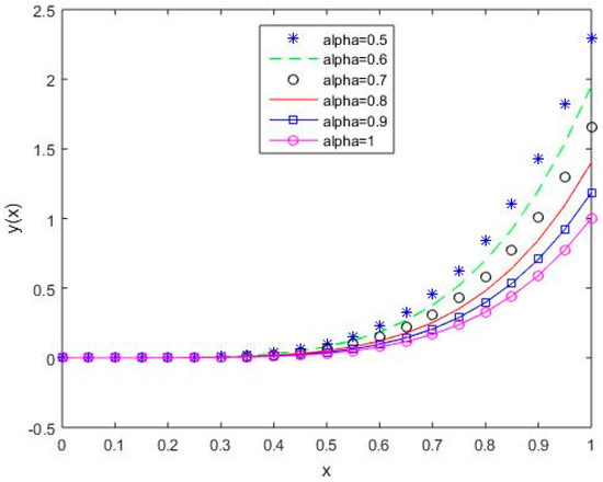
Figure 10. The behavior of solutions using S5 for $\alpha$ values of 0.5, 0.6, 0.7, 0.8, 0.9, and 1, Example 1.

In Table 1, we have listed the maximum absolute errors (MAE) and root-mean-square errors (RMSE) for Example 1 for the two different n values of 2 and 6.

Table 1. Result comparison of Example 1 for different orthogonal polynomials at different values of n.

Polynomials	Maximum Absolute Errors		Root-Mean-Square Errors
	n = 2	n = 6	n = 2	n = 6
S1	1.4584 × 10−1	1.8326 × 10−7	1.3923 × 10−2	2.4900 × 10−8
S2	1.6154 × 10−1	4.2127 × 10−7	2.0960 × 10−2	7.1127 × 10−8
S3	2.2296 × 10−1	3.6897 × 10−7	1.3179 × 10−2	3.3726 × 10−8
S4	4.1764 × 10−1	1.0973 × 10−6	3.2039 × 10−2	1.7307 × 10−7
S5	1.9055 × 10−1	3.1593 × 10−7	2.2138 × 10−2	4.2368 × 10−8

In Table 1, we have compared results for different polynomials, and it is observed that the results for Shifted Legendre polynomials and Gegenbauer polynomials are better than those for the other polynomials. It is also observed that the MAE and RMSE decrease with increasing n.

Example 2.

Consider a non-linear fractional variational problem as in Equation (1) with$g\left(x\right)=h\left(x\right)=e^{-vx}$; we then have the following non-linear fractional variational problem [19]:

$$J\left(y\right)={\int }_0^1{\left(e^{-vx}{D}^{\alpha }y\left(x\right)-v\left(I^{1-\alpha }y\left(x\right)+1\right)e^{-vx}\right)}^{2}dx$$

(57)

under the constraints

$$y\left(0\right)=0,I^{1-\alpha }y\left(1\right)=ϵ.$$

The exact solution of the above equation is given as

$$y_{exact}\left(x\right)=\left(e^{-1}\left(1+ϵ\right)-1\right)v^{-\alpha }\left({\displaystyle \sum _{k=0}^{\infty }}\frac{\left(k+1\right)}{\Gamma \left(k+\alpha +1\right)}{\left(vx\right)}^{k+\alpha }\right)+x^{\alpha -1}{E}_{1,\alpha }\left(vx\right)-\frac{x^{\alpha -1}}{\Gamma \left(\alpha \right)}$$

where$E_{a,b}\left(x\right)$is the Mittag-Leffler function of order$a$and$b$and is defined as

$$E_{a,b}\left(x\right)={\sum }_{k=0}^{\infty }\frac{x^k}{\Gamma \left(ak+b\right)}.$$

We discuss Example 2 for different $\alpha$ values of $0.5,0.6,0.7,0.8,0.9,\mathrm{and}$ 1 and $ϵ=2.$

In Figure 11, Figure 12, Figure 13, Figure 14 and Figure 15, it is shown that the solutions for the two different values of $\alpha =0.8\mathrm{and}\alpha =1$ coincide with the exact solutions for different orthogonal polynomials at n = 5.

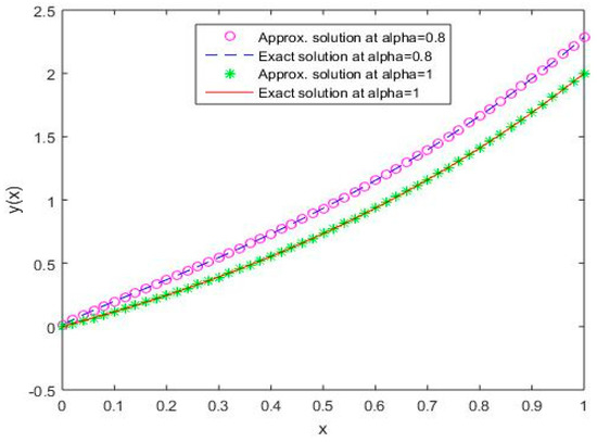
Figure 11. Comparison of exact and numerical solutions using S1 for $\alpha =0.8\mathrm{and}\alpha =1$, Example 2.

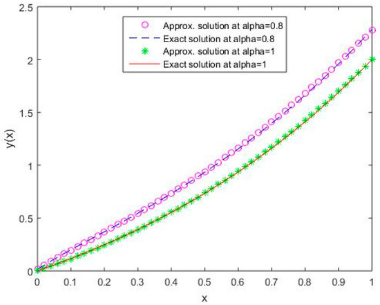
Figure 12. Comparison of exact and numerical solutions using S2 for $\alpha =0.8\mathrm{and}\alpha =1$, Example 2.

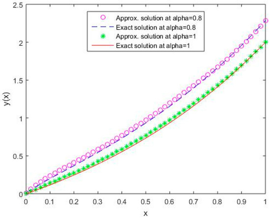
Figure 13. Comparison of exact and numerical solutions using S3 for $\alpha =0.8\mathrm{and}\alpha =1$, Example 2.

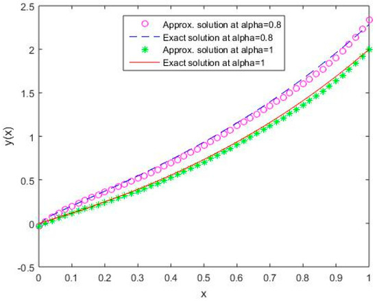
Figure 14. Comparison of exact and numerical solutions using S4 for $\alpha =0.8\mathrm{and}\alpha =1$, Example 2.

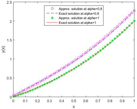
Figure 15. Comparison of exact and numerical solutions using S5 for $\alpha =0.8\mathrm{and}\alpha =1$, Example 2.

Figure 16, Figure 17, Figure 18, Figure 19 and Figure 20 reflect that the approximate solution varies continuously for Shifted Legendre polynomials, Shifted Chebyshev polynomials of the second kind, Shifted Chebyshev polynomials of the third kind, Shifted Chebyshev polynomials of the fourth kind, and Gegenbauer polynomials, respectively, with different values of fractional order.

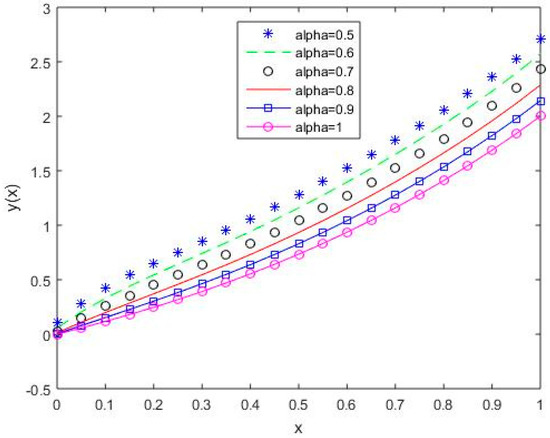
Figure 16. The behavior of solutions using S1 for $\alpha$ values of 0.5, 0.6, 0.7, 0.8, 0.9, and 1, Example 2.

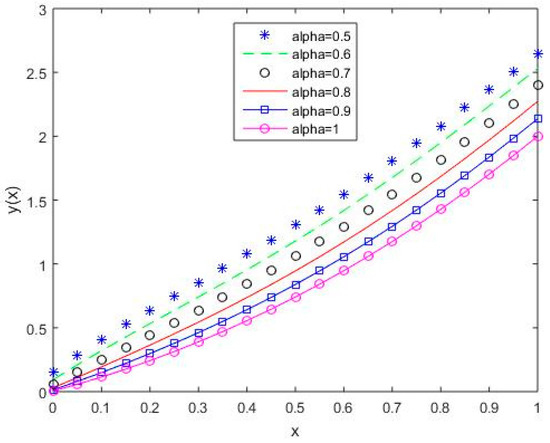
Figure 17. The behavior of solutions using S2 for $\alpha$ values of 0.5, 0.6, 0.7, 0.8, 0.9, and 1, Example 2.

Figure 18. The behavior of solutions using S3 for $\alpha$ values of 0.5, 0.6, 0.7, 0.8, 0.9, and 1, Example 2.

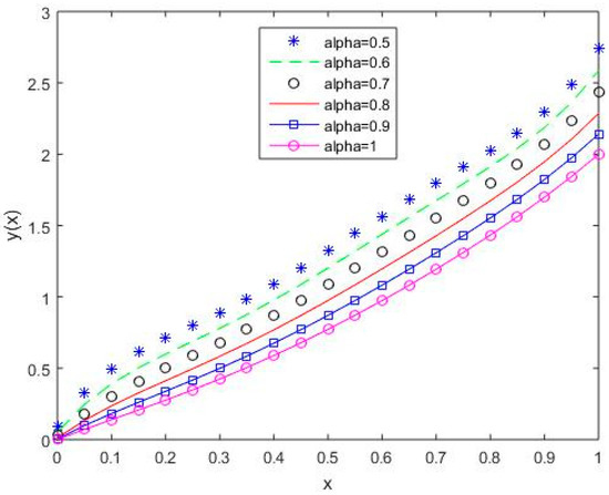
Figure 19. The behavior of solutions using S4 for $\alpha$ values of 0.5, 0.6, 0.7, 0.8, 0.9, and 1, Example 2.

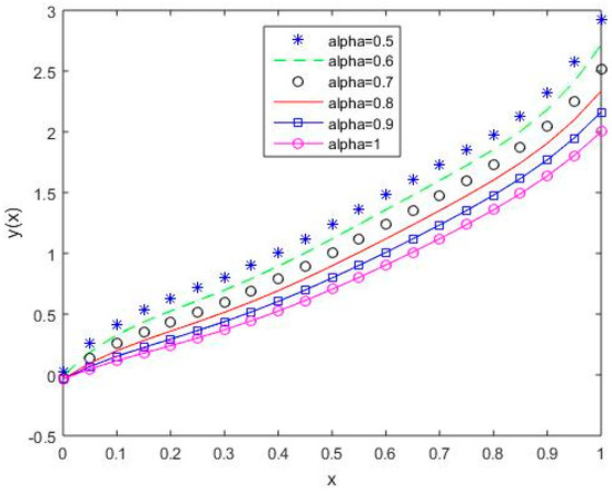
Figure 20. The behavior of solutions using S5 for $\alpha$ values of 0.5, 0.6, 0.7, 0.8, 0.9, and 1, Example 2.

In Table 2, we have listed the maximum absolute errors (MAE) and root-mean-square errors (RMSE) for Example 2 for the two n values 2 and 6.

Table 2. Result comparison of Example 2 for different orthogonal polynomials at different values of n.

Polynomials	Maximum Absolute Errors		Root-Mean-Square Errors
	n = 2	n = 6	n = 2	n = 6
S1	2.0407 × 10−2	1.4819 × 10−7	2.7038 × 10−3	1.5021 × 10−8
S2	2.4295 × 10−2	1.3713 × 10−2	3.1356 × 10−3	1.6490 × 10−3
S3	8.0010 × 10−2	4.8371 × 10−2	1.2590 × 10−2	8.3236 × 10−3
S4	1.1193 × 10−1	5.0558 × 10−2	9.8251 × 10−3	6.8594 × 10−3
S5	2.5349 × 10−2	1.9316 × 10−2	3.2343 × 10−3	2.4746 × 10−3

In Table 2, we have compared results for different polynomials, and it is observed that the results for the Shifted Legendre polynomial are better than those for the other polynomials. It is also observed that the MAE and RMSE decrease as $n$ increases.

8. Conclusions

We extended the Ritz method [18,20,21,22,32,33] for solving a class of NLFVPs using different orthogonal polynomials such as shifted Legendre polynomials, shifted Chebyshev polynomials of the first kind, shifted Chebyshev polynomials of the third kind, shifted Chebyshev polynomials of the fourth kind, and Gegenbauer polynomials. These polynomials were used to approximate the unknown function in the NLFVP. The advantage of the method is that it converts the given NLFVPs into a set of non-linear algebraic equations which are then solved numerically. The error bound of the approximation method for NLFVP was established. It was also shown that the approximate numerical solution converges to the exact solution as we increase the number of basis functions in the approximation. At the end, numerical results were provided by applying the method to two test examples, and it was observed that the results showed good agreement with the exact solution. Numerical results obtained using different orthogonal polynomials were compared. A comparative study showed that the shifted Legendre polynomials were more accurate in approximating the numerical solution.

References

- Dym, C.L.; Shames, I.H. Solid Mechanics: A Variational Approach; McGraw-Hill: New York, NY, USA, 1973. [Google Scholar]
- Frederico, G.S.F.; Torres, D.F.M. Fractional conservation laws in optimal control theory. Nonlinear Dyn. 2008, 53, 215–222. [Google Scholar] [CrossRef]
- Pirvan, M.; Udriste, C. Optimal control of electromagnetic energy. Balk. J. Geom. Appl. 2010, 15, 131–141. [Google Scholar]
- Agrawal, O.P. A general finite element formulation for fractional variational problems. J. Math. Anal. Appl. 2008, 337, 1–12. [Google Scholar] [CrossRef]
- Dehghan, M.; Tatari, M. The use of Adomian decomposition method for solving problems in calculus of variations. Math. Probl. Eng. 2006, 2006, 1–12. [Google Scholar] [CrossRef]
- Singh, H. A new stable algorithm for fractional Navier-Stokes equation in polar coordinate. Int. J. Appl. Comp. Math. 2017, 3, 3705–3722. [Google Scholar] [CrossRef]
- Robinson, A.D. The use of control systems analysis in neurophysiology of eye movements. Ann. Rev. Neurosci. 1981, 4, 462–503. [Google Scholar] [CrossRef] [PubMed]
- Singh, H. Operational matrix approach for approximate solution of fractional model of Bloch equation. J. King Saud Univ.-Sci. 2017, 29, 235–240. [Google Scholar] [CrossRef]
- Bagley, R.L.; Torvik, P.J. Fractional calculus a differential approach to the analysis of viscoelasticity damped structures. AIAA J. 1983, 21, 741–748. [Google Scholar] [CrossRef]
- Bagley, R.L.; Torvik, P.J. Fractional calculus in the transient analysis of viscoelasticity damped structures. AIAA J. 1985, 23, 918–925. [Google Scholar] [CrossRef]
- Panda, R.; Dash, M. Fractional generalized splines and signal processing. Signal Process. 2006, 86, 2340–2350. [Google Scholar] [CrossRef]
- Magin, R.L. Fractional calculus in bioengineering. Crit. Rev. Biomed. Eng. 2004, 32, 1–104. [Google Scholar] [CrossRef] [PubMed]
- Bohannan, G.W. Analog fractional order controller in temperature and motor control applications. J. Vib. Control. 2008, 14, 1487–1498. [Google Scholar] [CrossRef]
- Novikov, V.V.; Wojciechowski, K.W.; Komkova, O.A.; Thiel, T. Anomalous relaxation in dielectrics. Equations with fractional derivatives. Mater. Sci. 2005, 23, 977–984. [Google Scholar]
- Agrawal, O.P. A new Lagrangian and a new Lagrange equation of motion for fractionally damped systems. J. Appl. Mech. 2013, 237, 339–341. [Google Scholar] [CrossRef]
- Mozyrska, D.; Torres, D.F.M. Minimal modified energy control for fractional linear control systems with the Caputo derivative. Carpath. J. Math. 2010, 26, 210–221. [Google Scholar]
- Almeida, R.; Malinowska, R.; Torres, D.F.M. A fractional calculus of variations for multiple integrals with application to vibrating string. J. Math. Phys. 2010, 51, 033503. [Google Scholar] [CrossRef]
- Lotfi, A.; Dehghan, M.; Yousefi, S.A. A numerical technique for solving fractional optimal control problems. Comput. Math. Appl. 2011, 62, 1055–1067. [Google Scholar] [CrossRef]
- Khosravian-Arab, H.; Almeida, R. Numerical solution for fractional variational problems using the Jacobi polynomials. Appl. Math. Modell. 2015. [Google Scholar] [CrossRef]
- Agrawal, O.P. Formulation of Euler-Lagrange equations for fractional variational problems. J. Math. Anal. Appl. 2002, 272, 368–379. [Google Scholar] [CrossRef]
- Doha, E.H.; Bhrawy, A.H.; Baleanu, D.; Ezz-Eldien, S.S.; Hafez, R.M. An efficient numerical scheme based on the shifted orthonormal Jacobi polynomials for solving fractional optimal control problems. Adv. Differ. Equ. 2015. [Google Scholar] [CrossRef]
- Ezz-Eldie, S.S.; Doha, E.H.; Baleanu, D.; Bhrawy, A.H. A numerical approach based on Legendre orthonormal polynomials for numerical solutions of fractional optimal control problems. J. Vib. Ctrl. 2015. [Google Scholar] [CrossRef]
- Osama, H.M.; Fadhel, S.F.; Zaid, A.M. Numerical solution of fractional variational problems using direct Haar wavelet method. Int. J. Innov. Res. Sci. Eng. Technol. 2014, 3, 12742–12750. [Google Scholar]
- Ezz-Eldien, S.S. New quadrature approach based on operational matrix for solving a class of fractional variational problems. J. Comp. Phys. 2016, 317, 362–381. [Google Scholar] [CrossRef]
- Bastos, N.; Ferreira, R.; Torres, D.F.M. Discrete-time fractional variational problems. Signal Process. 2011, 91, 513–524. [Google Scholar] [CrossRef]
- Wang, D.; Xiao, A. Fractional variational integrators for fractional variational problems. Commun. Nonlinear Sci. Numer. Simul. 2012, 17, 602–610. [Google Scholar] [CrossRef]
- Odzijewicz, T.; Malinowska, A.B.; Torres, D.F.M. Fractional variational calculus with classical and combined Caputo derivatives. Nonlinear Anal. 2012, 75, 1507–1515. [Google Scholar] [CrossRef]
- Bhrawy, A.H.; Ezz-Eldien, S.S. A new Legendre operational technique for delay fractional optimal control problems. Calcolo 2015. [Google Scholar] [CrossRef]
- Tavares, D.; Almeida, R.; Torres, D.F.M. Optimality conditions for fractional variational problems with dependence on a combined Caputo derivative of variable order. Optimization 2015, 64, 1381–1391. [Google Scholar] [CrossRef]
- Ezz-Eldien, S.S.; Hafez, R.M.; Bhrawy, A.H.; Baleanu, D.; El-Kalaawy, A.A. New numerical approach for fractional variational problems using shifted Legendre orthonormal polynomials. J. Optim. Theory Appl. 2017, 174, 295–320. [Google Scholar] [CrossRef]
- Almeida, R. Variational problems involving a Caputo-type fractional derivative. J. Optim. Theory Appl. 2017, 174, 276–294. [Google Scholar] [CrossRef]
- Pandey, R.K.; Agrawal, O.P. Numerical Scheme for Generalized Isoparametric Constraint Variational Problems with A-Operator. In Proceedings of the ASME International Design Engineering Technical Conferences and Computers and Information in Engineering Conference, Portland, OR, USA, 4–7 August 2013. [Google Scholar] [CrossRef]
- Pandey, R.K.; Agrawal, O.P. Numerical scheme for a quadratic type generalized isoperimetric constraint variational problems with A.-operator. J. Comput. Nonlinear Dyn. 2015, 10, 021003. [Google Scholar] [CrossRef]
- Pandey, R.K.; Agrawal, O.P. Comparison of four numerical schemes for isoperimetric constraint fractional variational problems with A-operator. In Proceedings of the ASME 2015 International Design Engineering Technical Conferences and Computers and Information in Engineering Conference, Boston, MA, USA, 2–5 August 2015. [Google Scholar] [CrossRef]
- Singh, H.; Srivastava, H.M.D.; Kumar, D. A reliable numerical algorithm for the fractional vibration equation. Chaos Solitons Fractals 2017, 103, 131–138. [Google Scholar] [CrossRef]
- Singh, O.P.; Singh, V.K.; Pandey, R.K. A stable numerical inversion of Abel’s integral equation using almost Bernstein operational matrix. J. Quant. Spec. Rad. Trans. 2012, 111, 567–579. [Google Scholar] [CrossRef]
- Zhou, F.; Xu, X. Numerical solution of convection diffusions equations by the second kind Chebyshev wavelets. Appl. Math. Comput. 2014, 247, 353–367. [Google Scholar] [CrossRef]
- Yousefi, S.A.; Behroozifar, M.; Dehghan, M. The operational matrices of Bernstein polynomials for solving the parabolic equation subject to the specification of the mass. J. Comput. Appl. Math. 2011, 235, 5272–5283. [Google Scholar] [CrossRef]
- Singh, H. A New Numerical Algorithm for Fractional Model of Bloch Equation in Nuclear Magnetic Resonance. Alex. Eng. J. 2016, 55, 2863–2869. [Google Scholar] [CrossRef]
- Khalil, H.; Khan, R.A. A new method based on Legendre polynomials for solutions of the fractional two dimensional heat conduction equations. Comput. Math. Appl. 2014, 67, 1938–1953. [Google Scholar] [CrossRef]
- Singh, C.S.; Singh, H.; Singh, V.K.; Singh, O.P. Fractional order operational matrix methods for fractional singular integro-differential equation. Appl. Math. Modell. 2016, 40, 10705–10718. [Google Scholar] [CrossRef]
- Rivlin, T.J. An Introduction to the Approximation of Functions; Dover Publication: New York, NY, USA, 1981. [Google Scholar]
- Kreyszig, E. Introductory Functional Analysis with Applications; John Wiley and Sons, Inc.: Hoboken, NJ, USA, 1978. [Google Scholar]
- Bhrawy, A.H.; Tharwat, M.M.; Alghamdi, M.A. A new operational matrix of fractional integration for shifted Jacobi polynomials. Bull. Malays. Math. Sci. Soc. 2014, 37, 983–995. [Google Scholar]
- Behroozifar, M.; Sazmand, A. An approximate solution based on Jacobi polynomials for time-fractional convection–diffusion equation. Appl. Math. Comput. 2017, 296, 1–17. [Google Scholar] [CrossRef]
© 2019 by the authors. Licensee MDPI, Basel, Switzerland. This article is an open access article distributed under the terms and conditions of the Creative Commons Attribution (CC BY) license (http://creativecommons.org/licenses/by/4.0/).