1. Introduction
Clustering is the process of grouping homogeneous objects based on the correlation among similar attributes. This is useful in several common applications that require the discovery of hidden patterns among the collective data to assist decision making, e.g., bank transaction fraud detection [
1], market trend prediction [
2,
3] and a network intrusion detection system [
4]. Most traditional clustering algorithms developed rely on multiple iterations of evaluation on a fixed set of data to generate the clusters. However, in practical applications, these detection systems are operating daily, whereby millions of input data points are continuously streamed indefinitely, hence imposing speed and memory constraints. In such dynamic data stream environments, keeping track of every historical data would be highly memory expensive and, even if possible, would not solve the problem of analysing big data within the real-time requirements. Hence, a method of analysing and storing the essential information of the historical data in a single pass is mandatory for clustering data streams.
In addition, the dynamic data clustering algorithm needs to address two special characteristics that often occur in data streams, which are known as “
concept drift” and “
concept evolution” [
5]. Concept drift refers to the change of underlying concepts in the stream as time progresses, i.e., the change in the relationship between the attributes of the object within the individual clusters. For example, customer behaviour in purchasing trending products always changes in between seasonal sales. Meanwhile, concept evolution occurs when a new class definition has evolved in the data streams, i.e., the number of clusters has changed due to the creation of new clusters or the deprecation of old clusters. This phenomenon often occurs in the detection system whereby an anomaly has emerged in the data traffic. An ideal data stream clustering algorithm should address these two main considerations to detect and adapt effectively to changes in the dynamic data environment.
Based on recent literature, metaheuristics for black-box optimisation have been greatly adopted in traditional static data clustering [
6]. These algorithms have a general purpose application domain and often display self-adaptive capabilities, thus being able to tackle the problem at hand, regardless of its nature and formulation, and return near-optimal solutions. For clustering purposes, the so-called “population based” metaheuristic algorithms have been discovered to be able to achieve better global optimisation results than their “single solution” counterparts [
7]. Amongst the most commonly used optimisation paradigms of this kind, it is worth mentioning the established Differential Evolution (DE) framework [
8,
9,
10], as well as more recent nature inspired algorithms from the Swarm Intelligence (SI) field, such as the Whale Optimisation Algorithm (WOA) [
11] and the Bat-inspired algorithm in [
12], here referred to as BAT. Although the literature is replete with examples of data clustering strategies based on DE, WOA and BAT for the static domain, as, e.g., those presented in [
13,
14,
15,
16], little has been done for the dynamic environment due to the difficulties in handling data streams. The current state of dynamic clustering is therefore unsatisfactory as it mainly relies on algorithms based on techniques such as density microclustering and density grid based clustering, which require the tuning of several parameters to work effectively [
17].
This paper presents a methodology for integrating metaheuristic optimisation into data stream clustering, thus maximising the performance of the classification process. The proposed model does not require specifically tailored optimisation algorithms to function, but it is a rather general framework to use when highly dynamic streams of data have to be clustered. Unlike similar methods, we do not optimise the parameters of a clustering algorithm, but use metaheuristic optimisation in its initialisation phase, in which the first clusters are created, by finding the optimal position of their centroids. This is a key step as the grouped points are subsequently processed with the method in [
18] to form compact, but informative, microclusters. Hence, by creating the optimal initial environment for the clustering method, we make sure that the dynamic nature of the problem will not deteriorate its performances. It must be noted that microclusters are lighter representations of the original scenario, which are stored to preserve the “memory” of the past classifications. These play a major role since they aid subsequent clustering processes when new data streams are received. Thus, a non-optimal microclusters store in memory can have catastrophic consequences in terms of classification results. In this light, our original use of the metaheuristic algorithm finds its purpose, and results confirm the validity of our idea. The proposed clustering scheme efficiently tracks changes and spots patterns accordingly.
The remainder of this paper has the following structure:
Section 2 discusses the recent literature and briefly explains the logic behind the leading data stream clustering algorithms;
Section 3 establishes the motivations and objectives of this research and presents the used metaheuristic optimisation methods, the employed performance metrics and the considered datasets for producing numerical results;
Section 4 gives a detailed description of each step involved in the proposed clustering system, clarifies its working mechanism and shows methodologies for its implementation;
Section 5 describes the performance metrics used to evaluate the system and provides experimental details to reproduce the presented results;
Section 6 presents and comments on the produced results, including a comparison among different variants of the proposed system, over several evaluation metrics;
Section 7 outlines a thorough analysis of the impact of the parameter setting for the optimisation algorithm on the overall performance of the clustering system;
Section 8 summarises the conclusions of this research.
2. Background
There are two fundamentals aspects to take into consideration in data stream clustering, namely concept drift and concept evolution. The first aspect refers to the phenomenon when the data in the stream undergo changes in the statistical properties of the clusters with respect to the time [
19,
20] while the second to the event when there is an unseen novel cluster appearing in the stream [
5,
21].
Time window models are deployed to handle concept drift in data streams. These are usually embedded into clustering algorithms to control the quantity of historical information used in analysing dynamic patterns. Currently, there are four predominant window models in the literature [
22]:
the “damped time window” model, where historical data weights are dynamically adjusted by fixing a rate of decay according to the number of observations assigned to it [
23];
the “sliding time window” model, where only the most recent past data observations are considered with a simple First-In-First-Out (FIFO) mechanism. as in [
24];
the “landmark time window” model, where the data stream is analysed in batches by accumulating data in a fixed width buffer before being processed;
the “tilted time window” model, where the granularity level of weights gradually decreases as data points get older.
As for concept evolution, most of the existing data stream clustering algorithms are designed following a two phase approach, i.e., consisting of an online clustering process followed by an offline one, which was first proposed in [
25]. In this work, the concept of microclusters was also defined to design the so-called CluStream algorithm. This method forms microclusters having statistical features representing the data stream online. Similar microclusters are then merged into macro-clusters, keeping only information related to the centre of the densest region. This is performed offline, upon user request, as it comes with information losses since merged clusters can no longer be split again to obtain the original ones.
In terms of online microclustering, most algorithms in the literature are distance based [
17,
22,
26], whereby new observations are either merged with existing microclusters or form new microclusters based on a distance threshold. The earliest form of distance based clustering strategy was the process of extracting information about a cluster into the form of a Clustering Feature (CF) vector. Each CF usually consists of three main components: (1) a linear combination of the data points referred to as Linear Sum vector
; (2) a vector
whose components are the Squared Sums of the corresponding data points’ components; (3) the number N of points in a cluster.
As an instance, the popular CluStream algorithm in [
25] makes use of CF and the tilted time window model. During the initialisation phase, data points are accumulated to a certain amount before being converted into some microclusters. On the arrival of new streams, new data are merged with the closest microclusters if their distance from the centre of the data point to the centre of the microclusters is within a given radius (i.e., the
-neighbourhood method). If there is no suitable microclusters within this range, a new microclusters is formed. When requested, the CluStream uses the k-means algorithm [
27] to generate macroclusters from microclusters in its offline phase. It also implements an ageing mechanism based on timestamps to remove outdated clusters from its online components.
Another state-of-the-art algorithm, i.e. DenStream, was proposed in [
18] as an extension of CluStream using the damped time window and a novel clustering strategy named “time-faded CF”. DenStream separates the microclusters into two categories: the potential core microclusters (referred to as p-microclusters) and the outlier microclusters (referred to as o-microclusters). Each entry of the CF is subject to a decay function that gradually reduces the weight of each microcluster at a regular evaluation interval period. When the weight falls below a threshold value, the affected p-microclusters are degraded to the o-microclusters, and they are removed from the o-microclusters if the weights deteriorate further. On the other hand,o-microclusters that have their weights improved are promoted to p-microclusters. This concept allows new and old clusters to form online gradually, so addressing the concept evolution issue. In the offline phase, only the p-microclusters are used for generating the final clusters. Similar p-microclusters are merged employing a density based approach based on the
-neighbourhood method. Unlike other commonly used methods, in this case, clusters can assume an arbitrary shape, and no a priori information is needed to fix the number of clusters.
An alternative approach was given in [
28], where the proposed STREAM algorithm did not store CF vectors, but directly computed centroids on-the-fly. This was done by solving the “k-means clustering” problem to identify the centroids of
K clusters. The problem was structured in a form whereby the distance from data points to the closest cluster had associated costs. Using this framework, the clustering task was defined as a minimisation problem to find the number and position of centroids that yielded the lowest costs. To process an indefinite length of streaming data, the landmark time window was used to divide the streams into
n batches of data, and the
K-means problem solving was performed on each chunk. Although the solution was plausible, the algorithm was evaluated to be time consuming and memory expensive in processing streaming data.
The OLINDDA method proposed in [
29] extends the previously described centroid approach by integrating the
-neighbourhood concept. This was used to detect drifting and new clusters in the data stream, with the assumption that drift changes occurred within the existing cluster region, whilst new clusters formed outside the existing cluster region. The downside of the centroid approach was that the number of
K centroids needed to be known a priori, which is problematic in a dynamic data environment.
There is one shortcoming for the two phase approach, i.e., the ability to track changes in the behaviour of the clusters is linearly proportional to the frequency of requests for the offline component [
30]. In other words, the higher the sensitivity to changes, the higher the computational cost. To mitigate these issues, an alternative approach has been explored by researchers to merge these two phases into a single online phase. FlockStream [
31] deploys data points into a virtual mapping of a two-dimensional grid, where each point is represented as an agent. Each agent navigates around the virtual space according to a model mimicking the behaviour of flocking birds, as done in the most popular SI algorithms, e.g., those in [
32,
33,
34]. The agent behaviour was designed in a way such that similar (according to a given metric) birds would move in the same direction as the closest neighbours, forming different groups of the flock. These groups can be seen as clusters, thus eliminating the need for a subsequent offline phase.
MDSC [
35] is another single phase method exploiting the SI paradigm inspired by the density based approached introduced in DenStream. In this method, the Ant Colony Optimisation (ACO) algorithm [
36] is used to group similar microclusters optimally during the online phase. In MDSC, a customised
-neighbourhood value is assigned to each cluster to enable “multi-density” clusters to be discovered.
Finally, it is worth mentioning the ISDI algorithm in [
37], which is equipped with a windowing routine to analyse and stream data from multiple sources, a timing alignment method and a deduplication algorithm. This algorithm was designed to deal with data streams coming from different sources in the Internet of Things (IoT) systems and can transform multiple data streams, having different attributes, into cleaner datasets suitable for clustering. Thus, it represents a powerful tool allowing for the use of streams classifiers, as, e.g., the one proposed in this study, in IoT environments.
3. Motivations, Objectives and Methods
Clustering data streams is still an open problem with room for improvement [
38]. Increasing the classification efficiency in this dynamic environment has a great potential in several application fields, from intrusion detection [
39] to abnormality detection in patients’ physiological data streams [
40]. In this light, the proposed methodology draws its inspiration from key features of the successful methods listed in
Section 2, with the final goal of improving upon the current state-of-the-art.
A hybrid algorithm is then designed by employing, along with standard methods, as, e.g., CF vectors and the landmark time windows model, modern heuristic optimisation algorithms. Unlike similar approaches available in the literature [
36,
41,
42], the optimisation algorithm is here used during the online phase to create optimal conditions for the offline phase. This novel approach is described in detail in
Section 4.
To select the most appropriate optimisation paradigm, three widely used algorithms, i.e., WOA, BAT and DE, were selected from the literature and compared between them. We want to clarify that the choice of using three metaheuristic methods, rather than other exact or iterative techniques, was made to be able to deal with the challenging characteristics of the optimisation problem at hand, e.g., the dimensionality of the problem can vary according to the dataset, and the objective functions is highly non-linear and not differentiable, which make them not applicable or time inefficient.
A brief introduction of the three selected algorithms is given below in
Section 3.1. Regardless of the specific population based algorithm used for performing the optimisation step, each candidate solution must be encoded as an
n-dimensional real valued vector representing the
K cluster centres for initialising the following density based clustering method.
Two state-of-the-art deterministic data stream clustering algorithms, namely DenStream and CluStream, are also included in the comparative analysis to further validate the effectiveness of the proposed framework.
The evaluation methodology employed in this work consisted of running classification experiments over the datasets in
Section 3.2 and measuring the obtained performances through the metrics defined in
Section 3.3.
3.1. Metaheuristic Optimisation Methods
This section gives details on the implementation of the three optimisation methods used to test the proposed system.
3.1.1. The Whale Optimization Algorithm
The WOA algorithm is a swarm based stochastic metaheuristic algorithm inspired by the hunting behaviour of humpback whales [
11]. It is based on a mathematical model updated by iterating the three search mechanisms described below:
the “shrinking encircling prey” mechanism is exploitative and consists of moving candidate solutions (i.e., the whales) in a neighbourhood of a the current best solution in the swarm (i.e., the prey solution) by implementing the following equation:
where: (1)
is linearly decreased from two to zero as iterations increase (to represent shrinking, as explained in [
7]); (2)
is a vector whose components are randomly sampled from
(
t is the iteration counter); (3) the “*” notation indicates the pairwise products between two vectors.
the “spiral updating position” mechanism is also exploitative and mimics the swimming pattern of humpback whales towards prey in a helix shaped form through Equations (
2) and (
3):
with:
where
b is a constant value for defining the shape of the logarithmic spiral;
l is a random vector in
; the “
” symbol indicates the absolute value of each component of the vector;
the “search for prey” mechanism is exploratory and uses a randomly selected solution
as an “attractor” to move candidate solutions towards unexplored areas of the search space and possibly away from local optima, according to Equations (
4) to (
5):
with:
The reported equations implemented a search mechanism that mimics movements made by whales. Mathematically, it is easier to understand that some of them refer to explorations moves across the search space, while others are exploitation moves to refine solutions within their neighbourhood. To have more information on the metaphor inspiring these equations, their formulations and their role in driving the research within the algorithm framework, one can see the survey article in [
6]. A detailed scheme describing the coordination logic of the three previously described search mechanism is reported in Algorithm 1.
| Algorithm 1 WOA pseudocode. |
- 1:
Generate initial whale positions , where - 2:
Compute the fitness of each whale solution, and identify - 3:
whiledo - 4:
for do - 5:
Update - 6:
if then - 7:
if then - 8:
Update the position of current whale using Equation ( 1) - 9:
else if then - 10:
- 11:
Update the position of current whale with Equation ( 4) - 12:
end if - 13:
else if then - 14:
Update the position of current whale with Equation ( 2) - 15:
end if - 16:
end for - 17:
Calculate new fitness values - 18:
Update - 19:
- 20:
end while - 21:
Return
|
With reference to Algorithm 1, the initial swarm is generated by randomly sampling solutions in the search; the best solution is kept up to date by replacing it only when an improvement on the fitness value occurs; the optimisation process lasts for a prefixed number of iterations, here indicated with max budget; the probability of using the shrinking encircling rather than the spiral updating mechanism was fixed at 0.5.
3.1.2. The BAT Algorithm
The BAT algorithm was a swarm based searching algorithm inspired by the echolocation abilities of bats [
12]. Bats use sound wave emissions to generate an echo that measures the distance of its prey based on the loudness and time difference of the echo and sound wave. To reproduce this system and exploit it for optimisation purposes, the following perturbation strategy must be implemented:
where
is the position of the candidate solution in the search space (i.e., the bat),
is its velocity,
is referred to as the “wave frequency” factor and
is a random vector in
(where
n is the dimensionality of the problem).
and
represent the lower and upper bounds of the frequency, respectively. Typical values are within 0 and 100. When the bat is close to the prey (i.e., current best solution), it gradually reduces the loudness of its sound wave while increasing the pulse rate. The pseudocode depicted in Algorithm 2 shows the the working mechanism of the BAT algorithm.
| Algorithm 2 BAT pseudocode. |
- 1:
Generate initial bats () and their velocity vectors - 2:
Compute the fitness values, and find - 3:
Initialise pulse frequency at - 4:
Initialise pulse rate and loudness - 5:
whiledo - 6:
for do - 7:
move to a new position with Equations ( 6)–( 8) - 8:
end for - 9:
for do - 10:
if then - 11:
added with a random - 12:
end if - 13:
if and improved then - 14:
- 15:
Increase and decrease - 16:
end if - 17:
end for - 18:
Update - 19:
- 20:
end while - 21:
Return
|
To have more detailed information on the equations used to perturb the solutions within the search space in the BAT algorithm, we suggest reading [
43].
3.1.3. The Differential Evolution
The Differential Evolution (DE) algorithms are efficient metaheuristics for global optimisation based on a simple and solid framework, first introduced in [
8], which only requires the tuning of three parameters, namely the scale factor
, the crossover ratio
and the population size
. As shown in Algorithm 3, despite using crossover and mutation operators, which are typical of evolutionary algorithms, it does not require any selection mechanism as solutions are perturbed one at a time by means of the one-to-one spawning mechanising from the SI field. Several DE variants can be obtained by using different combinations of crossover and mutation operators [
44]. The so-called “DE/best/1/bin” scheme was adopted in this study, which employs the best mutation strategy and the binomial crossover approach. The pseudocode and other details regarding these operators are available in [
10].
| Algorithm 3 DE pseudocode. |
- 1:
Generate initial population with - 2:
Compute the fitness of each individual, and identify - 3:
whiledo - 4:
for do - 5:
▹ “best/1” as explained in [ 10] - 6:
▹ “bin” as explained in [ 10] - 7:
Store the best individual between and in the position of a new population - 8:
end for - 9:
end - 10:
Replace the current population with the newly generated population - 11:
Update - 12:
end while - 13:
Return
|
3.2. Datasets
Four synthetic datasets were generated using the built-in stream data generator of the “Massive Online Analysis” (MOA) software [
45]. Each synthetic dataset represents different data streaming scenarios with varying dimensions, clusters numbers, drift speed and frequency of concept evolution. These datasets are:
the 5C5Cdataset, which contains low-dimensional data with a low rate of data changes;
the 5C10C dataset, which contains low-dimensional data with a high rate of data changes;
the 10D5C dataset, which is a 5C5C variant containing high-dimensional data;
the 10D10C dataset, which is a 5C10C variant containing high-dimensional data.
Moreover, the KDD-99 dataset [
46], containing real network intrusion information, was also considered in this study. It must be highlighted that the original KDD-99 dataset contained 494,021 data entries, representing network connections generated in military network simulations. However, only 10% of the entries were randomly selected for this study. Each data entry contained 41 features and one output column to distinguish the attack connection from the normal network connection. The attacks can be further classified into 22 attack types. Streams are obtained by reading each entry of the dataset sequentially.
Details on the five employed datasets are given in
Table 1.
3.3. Performance Metrics
To perform an informative comparative analysis, three metrics were cherry picked from the data stream analysis literature [
41,
42]. These are referred to as the F-measure, purity and Rand index [
47].
Mathematically, these metrics are expressed with the following equations:
where:
and:
C is the solution returned by the clustering algorithm (i.e., the number of clusters k);
is the the ith cluster ();
is the class label with the highest frequency in ;
is the number of instances labelled with in ;
is the total number of instances identified in the totality of clusters returned by the algorithm.
The F-measure represents the harmonic mean of the precision and recall scores, where the best value of one indicates ideal precision and recall, while zero is the worst scenario.
Purity is used to measure the homogeneity of the clusters. Maximum purity is achieved by the solution when each cluster only contains a single class.
The Rand index computes the accuracy of the clustering solution from the actual solution, based on the ratio of correctly identified instances among all the instances.
4. The Proposed System
This article proposes “OpStream”, an Optimised Stream clustering algorithm. This clustering framework consisted of two main parts: the initialisation phase and the online phase.
During the initialisation phase, a number of data points are accumulated through a landmark time window, and the unclassified points are initialised into groups of clusters via the centroid approach, i.e., generating K centroids of clusters among the points.
In the initialisation phase, the landmark time window is used to collect data points, which are subsequently grouped into clusters by generating K centroid. The latter are generated by solving K-centroid cost optimisation problems with a fast and reliable metaheuristic for optimisation. Hence, their position is optimal and leads to high quality predictions.
Next, during the online phase, the clusters are maintained and updated using the density based approach, whereby incoming data points with similar attributes (i.e., according to the -neighbourhood method) form dense microclusters in between two data buffers, namely p-microclusters and o-microclusters. These are converted into microclusters with CF information to store a “light” version of previous scenarios in this dynamic environment.
In this light, the proposed framework is similar to advanced single phase methods. However, it requires a preliminary optimisation process to boost its classification performances.
Three variants of OpStream were tested by using the three metaheuristic optimisers described in
Section 3. These stochastic algorithms (as the optimisation process is stochastic) are compared against the two DenStream and CluStream state-of-the-art deterministic stream clustering algorithms.
The following sections describe each step of the OpStream algorithm.
4.1. The Initialisation Phase
This step can be formulated as a real valued global optimisation search problem and addressed with the metaheuristic of black-box optimisation. To achieve this goal, a cost function must be designed to allow for the individualisation of the optimal position of the centroid of a cluster. These processes have to be iterated K times to then form K clusters by grouping data according to their distance from the optimal centroids.
The formulation of the cost function plays a key part. In this research, the “Cluster Fitness” (CF) function from [
48] was chosen as its maximisation leads to a high intra-cluster distance, which is desirable. Its mathematical formulation, for the
(
) cluster, is given below:
from where it can be observed that it is computed by averaging the
K clusters’ silhouettes “
”. These represent the average dissimilarity of all the points in the cluster and are calculated as follows
where
and
are the “inner dissimilarity” and the “outer dissimilarity”, respectively.
The former value measures the average dissimilarity between a data point
i and other data points in its own cluster
. Mathematically, this is expressed as:
with
being the Euclidean distance between the two points and
is the total number of points in cluster
. The lower the value, the better the clustering accuracy.
The latter value measures the minimum distance between a data point
i to the centre of all clusters, excluding its own cluster
. Mathematically, this is expressed as:
where
is the number of points in cluster
. The higher the value, the better the clustering.
These two values are contained in , whereby one indicates the ideal case and the most undesired one.
A similar observation can be done for the fitness function
[
48]. Hence, the selected metaheuristics have to be set up for a maximisation problem. This is not an issue since every real valued problem of this kind can be easily maximised with an algorithm designed for minimisation purposes by simply timing the fitness function by
, and vice versa.
Regardless of the dimensionality of the problem
n, which depends on the dataset (as shown in
Table 1), all input data were normalised within
. Thus, the search space for all the optimisation process was the hyper-cube defined as
.
4.2. The Online Phase
Once the initial clusters have been generated, by optimising the cost function formulated in
Section 4.1, clustered data points must be converted into microclusters. This step requires the extraction of CF vectors. Subsequently, a density based approach was used to cluster the data stream online.
4.2.1. Microclusters’ Structure
In OpStream, each CF must contain four components, i.e., CF N, , , timestamp], where
From CF, the centre
c and radius
r of a microclusters are computed as follows:
as indicated in [
18,
42].
The obtained
r value is used to initialise the
-neighbourhood approach (i.e.,
), leading to the formation of microclusters as explained in
Section 2. This microclusters, which are derived from a cluster formed in the initialisation phase, is now stored in the p-microclusters buffer.
4.2.2. Handling Incoming Data Points
In OpStream, for each new time window, a data point
p is first converted into a “degenerative” microcluster
containing a single point and having the following initial CF properties:
Subsequently, initial microclusters have to be merged. This task can efficiently be addressed by considering pairs of microclusters, say, e.g.,
and
, and computing their Euclidean distance
. If
is the cluster to be merged, its radius
r must be worked out as shown in
Section 4.2.1 and then be merged with
if:
Two microclusters satisfying the condition expressed with Equation (
22) are said to be “density reachable”. The process described above is repeated until there are no longer density reachable microclusters. Every time two microclusters are merged, e.g.,
and
, the CF properties of the newly generated microclusters, e.g.,
, are assigned as follows:
where
T is the time at which the two microclusters were merged.
When the condition in Equation (
22) is no longer met by a microcluster, this is moved to the p-microclusters buffer. If the newly added microclusters and other clusters in the p-microclusters buffer are density reachable, then they are merged. Otherwise, a new independent cluster is stored in this buffer.
This mechanism is performed by a software agent, referred to as the “Incoming Data Handler” (IDH), whose pseudocode is reported in Algorithm 4 to further clarify this process and allow for its implementation.
| Algorithm 4 IDH pseudocode. |
- 1:
Input: Data point p - 2:
Convert p into microcluster - 3:
Initialise - 4:
forin p-microclusters do - 5:
if then - 6:
if is density reachable to then - 7:
if new radius then - 8:
Merge with - 9:
else - 10:
Add to p-microclusters - 11:
end if - 12:
- 13:
end if - 14:
end if - 15:
end for - 16:
ifthen - 17:
for each in o-microclusters do - 18:
if then - 19:
if is density reachable to then - 20:
if new radius then - 21:
Merge with - 22:
- 23:
end if - 24:
end if - 25:
end if - 26:
end for - 27:
end if - 28:
ifthen - 29:
Add to o-microclusters - 30:
end if - 31:
end - 32:
return
|
4.2.3. Detecting and Forming New Clusters
Once microclusters in the o-microclusters buffer are all merged, as explained in
Section 4.2.2, only the minimum possible number of microclusters with the highest density exists. The microclusters with the highest number of points N is then moved to an empty set
C to initialise a new cluster. After calculating its centre
c, with Equation (
20), and radius
r, with Equation (
21), the
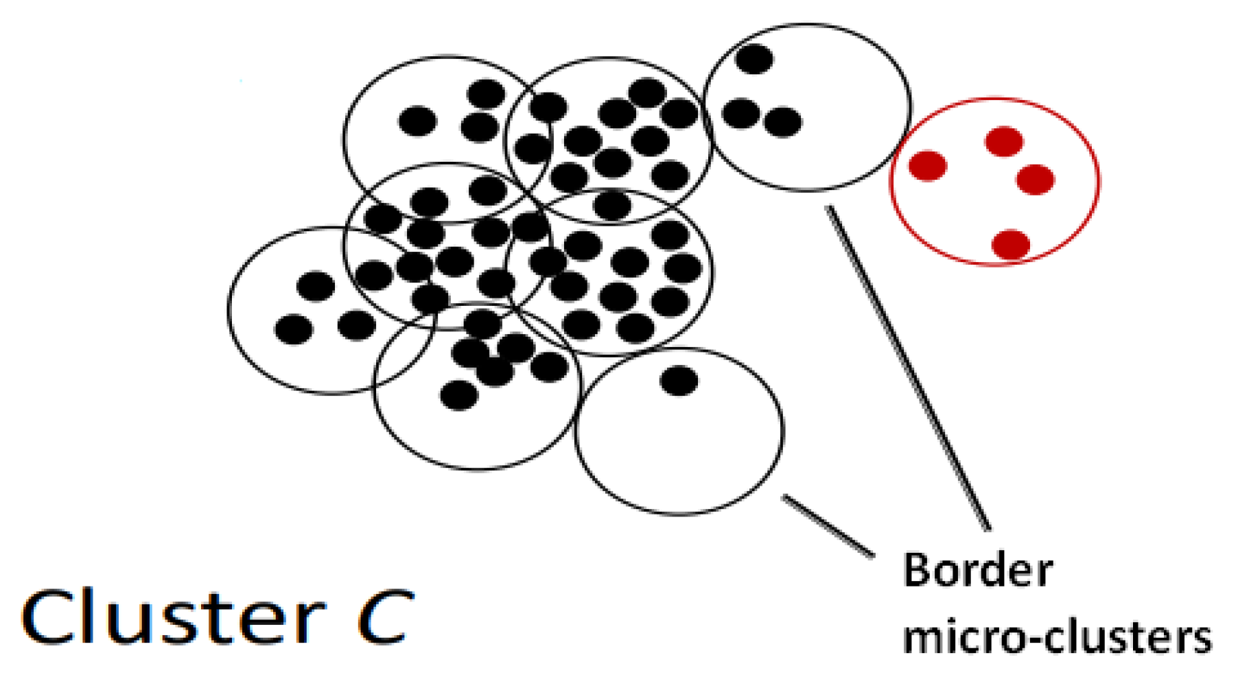
-neighbourhood method is again used to find density reachable microclusters. Among them, a process is undertaken to detect the so-called border microclusters [
35] inside C, which obviously are not present during the first iteration as
C initially contains only one microcluster. Border microclusters are defined as density reachable microclusters that have a density level that is below the density threshold of the first microclusters present in C. Having a threshold that is too high, cluster C will not expand, whilst having a value that is too low, cluster C will contain dissimilar microclusters. Based on the experimental data from the original paper [
35], a 10% threshold yields good performance.
Once the border microclusters are identified, only surrounding microclusters that are density reachable to the non-border microclusters are moved to form part of C, according to the process indicated in
Section 4.2.2.
Figure 1 graphically depicts C. The microclusters marked in red colour do not form as part of C because it is density reachable only to border microclusters of C.
This process is iterated as shown in Algorithm 5. The final version of
C is finally moved to the most appropriate buffer according to its size, i.e., if “
C.N ≥ minClusterSize”, all its microclusters are merged together, and the newly generated cluster
C is moved to the p-microclusters buffer. If this does not occur, the cluster
C is not generated by merging its microclusters, but they are simply left in the o-microclusters buffer. The recommended method to fix the minClusterSize parameter is:
These tasks are performed by the New Cluster Generator (NCG) software agent, whose pseudocode is shown in Algorithm 5.
| Algorithm 5 New cluster generation pseudocode. |
- 1:
Input: o-microclusters - 2:
while o-microclusters is not empty do - 3:
Initialise cluster C using with highest N - 4:
addedMc = true - 5:
while addedMc is true do - 6:
addedMc = false - 7:
for in o-microclusters do - 8:
if is density reachable to any non-border mc in C then - 9:
Add into C - 10:
Remove from o-microclusters - 11:
addedMc = true - 12:
end if - 13:
end for - 14:
end while - 15:
if the size of C is ≥ minClusterSize then ▹ minClusterSize is initialised with Equation ( 23) - 16:
Merge microclusters in C - 17:
Add C into p-microclusters - 18:
end if - 19:
end while
|
4.3. OpStream General Scheme
The proposed OpStream method involves the use of several techniques, such as metaheuristic optimisation algorithms, density based and k-means clustering, etc., and requires a software infrastructure coordinating activities as those performed by the IDH and NCG agents. Its architecture is outlined with the pseudocode in Algorithm 6.
| Algorithm 6 OpStream pseudocode |
. - 1:
Launch AS ▹ initialised with Equation ( 24) - 2:
initialisedFlag = false - 3:
while stream do - 4:
Add data point p into window - 5:
if initialisedFlag is true then - 6:
Handle incoming data streams with IDH, ▹ i.e., Algorithm 4 - 7:
end if - 8:
if window is full then - 9:
if initialisedFlag is false then - 10:
Optimise centres’ positions, and initialise clusters ▹ e.g., with Algorithm 1, 2 or 3 - 11:
initialisedFlag = true - 12:
else - 13:
Look for and generate new clusters with NCG, ▹ i.e., Algorithm 5 - 14:
end if - 15:
end if - 16:
end while
|
It must be added that an Ageing System (AS) is constantly run to remove outdated clusters. Despite its simplicity, its presence is crucial in dynamic environments. An integer parameter
(equal to four in this study) is used to compute the age threshold as shown below:
so that if a microcluster has not been updated in four consecutive windows, it will be removed from the respective buffer.
5. Experimental Setup
As discussed in
Section 3, OpStream’s performances were evaluated across four synthetic datasets and one real dataset using three popular performance metrics. Two deterministic state-of-the-art stream clustering algorithms, i.e., DenStream [
18] and CluStream [
25], were also run with the suggested parameter settings available in their original articles for caparison purposes.
The WOA algorithm was initially picked to implement the OpStream framework, as this framework is currently being intensively exploited for classification purposes, but two more variants employing BAT and DE (as described in
Section 3) were also run to: (1) show the flexibility of OpStream in the use of different optimisation methods; (2) display its robustness and superiority to deterministic approaches regardless of the optimiser used; (3) establish the preferred optimisation method over the specific datasets considered in this study. For the sake of clarity, these three variants are referred to as WOAS-OpStream, BAT-OpStream and DE-OpStream to represent the respective metaheuristic optimiser used. To reproduce the results presented in this article, the employed parameter setting of each metaheuristic, as well as other algorithmic details are reported below:
WOA: swarm Size ;
BAT: swarm size , , , , ();
DE: population Size = 20, , ;
the “max Iterations” value is set to 10 for all three algorithms to ensure a fair comparison (the computational budget was purposely kept low due to the real-time nature of the problem);
the three optimisation algorithms were equipped with the “toroidal” correction mechanism to handle infeasible solutions, i.e., solutions generated outside of the search space (a detailed description of this operator is available in [
10]).
Furthermore, the following parameter values were also required to run the OpStream framework:
Section 7 explains the role played by these parameters and how their suggested values were determined.
Thus, a total of five clustering algorithms was considered in the experimentation phase. These were executed, with the aid of the MOA platform [
45], 30 times over each dataset (the instances’ order was randomly changed for each repetition) to produce, for each evaluation metric, average ± standard deviation values. To further validate our conclusions statistically, the outcome of the Wilcoxon rank-sum test [
49] (with the confidence level equal to
) is also reported in all tables with the compact notation obtained from [
50], where (1) a “+” symbol next to an algorithm indicates that it was outperformed by the reference algorithm (i.e., WOA-OpStream); (2) a “−” symbol indicates that the reference algorithm was outperformed; (3) a “=” symbol shows that the two stochastic optimisation processes were statistically equivalent.
6. Results and Discussion
A table was prepared for each evaluation metric, each one displaying the average value, standard deviation and the outcome of the Wilcoxon rank-sum test (W) over the 30 performed runs. The best performance on each dataset is highlighted in boldface.
Table 2 reports the results in terms of the F-measure. According to this metric, the three OpStream variants generally outperformed the deterministic algorithms. The only exception is registered over the
KDDC–99 dataset, where DenStream displayed the best performance. From the statistical point of view, WOA-OpStream was significantly better than CluStream (with five “+” out of five cases), clearly preferable to DenStream (with four “+” out of five cases), equivalent to the DE-OpStream variant and approximately equivalent to BAT-OpStream.
Similarly, regarding
Table 3, WOA-OpStream showed a slightly better statistical behaviour than BAT-OpStream, and it was statistically equivalent to DE-OpStream, also in terms of purity. However, according to this metric, the stochastic classifiers did not outperform the deterministic ones, but had quite similar performances. In terms of the average value over the 30 repetitions, DE-OpStream and DenStream had the highest purity.
Finally, the same conclusions obtained with the F-measure were drawn by interpreting the results in
Table 4, where the Rand index metric was used to evaluate the classification performances. Indeed, all three OpStream variants statistically outperformed the deterministic methods. This goes to show that the proposed method was performing very well regardless of the optimisation strategy, and it was always better or competitive with state-of-the-art algorithms. Unlike the case in
Table 2, the best performances were in terms of the average value or those obtained with DE rather than WOA. However, the difference between the two variants was minimal, and the Wilcoxon rank-sum test did not detect differences between the two variants.
Summarising, OpStream displayed the best global performance, with WOA-OpStream and DE-OpStream being the most preferable variants. Statistically, WOA-OpStream and DE-OpStream had equivalent performances over different datasets and according to three different evaluation metrics. In this light, the WOA variant was preferred as it required the tuning of only two parameters, against the three required in DE, to function optimally.
A final observation can be done by separating the results from the synthetic datasets and
KDDC–99. If in the first case, the supremacy of OpStream was evident; a deterioration of the performances can be noted when the later dataset was used. In this light, one can understand that the proposed method presented room for improvement of handling data streams with an uneven distribution of class instances as those presented in
KDDC–99 [
51].
7. Further Analyses
In the light of what was observed in
Section 6, the WOA algorithm was preferred over DE and BAT to perform the optimisation phase. Hence, it was reasonable to consider the WOA-OpStream variant as the default OpStream algorithm implementation.
This section concludes this research with a thorough analysis of this variant in terms of sensitivity, scalability, robustness and flexibility to handle overlapping multi-density clusters.
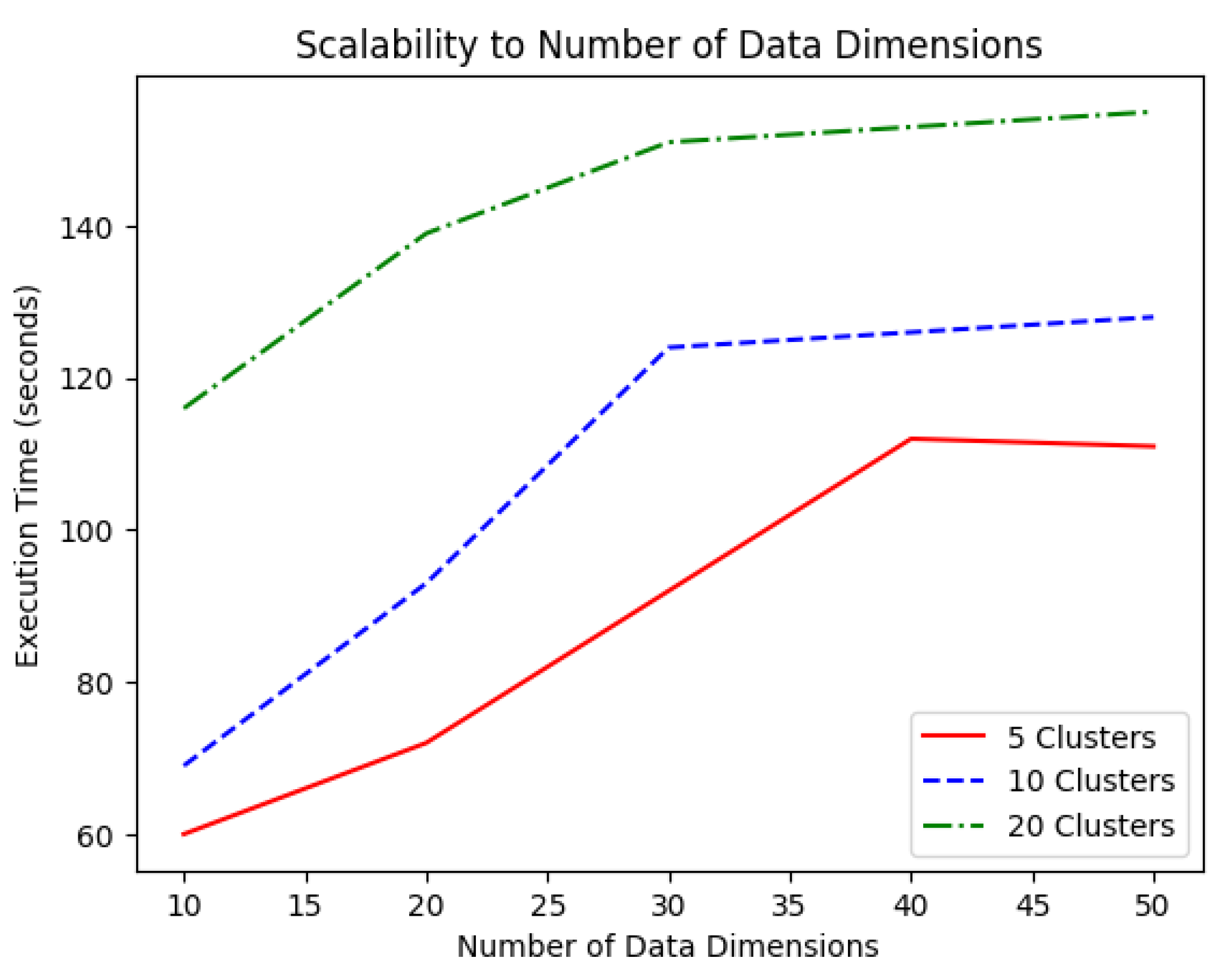
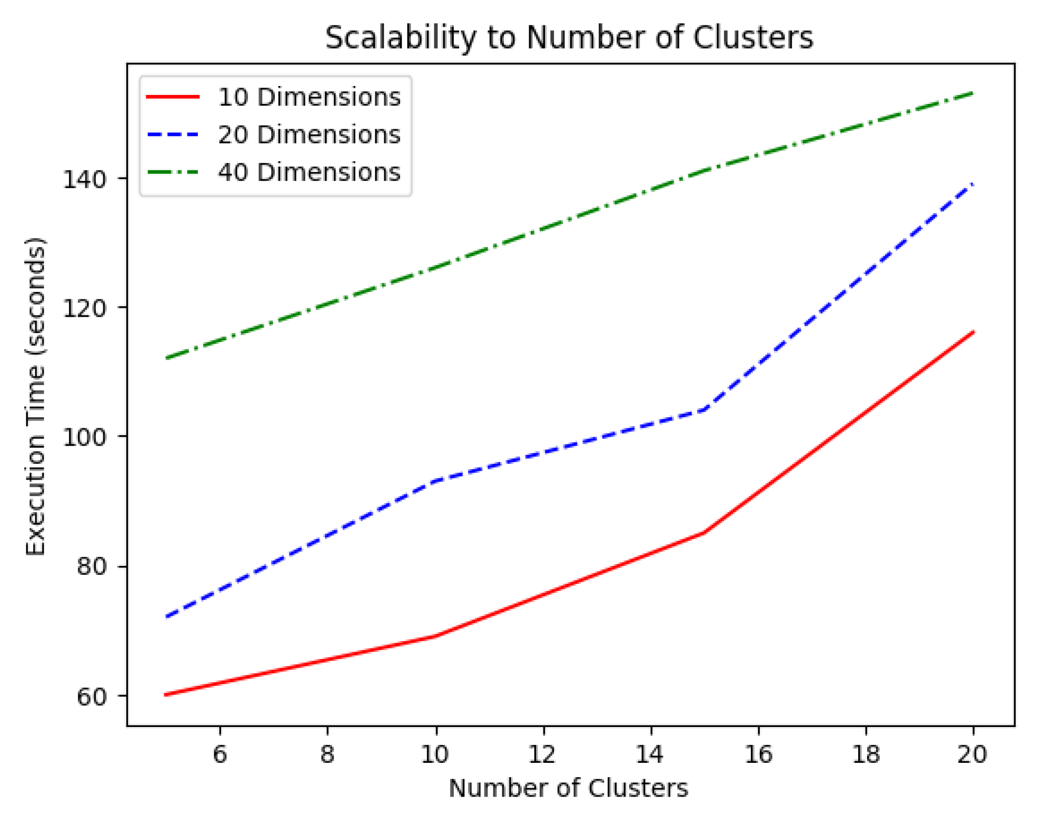
7.1. Scalability Analysis
A scalability analysis was performed to test how OpStream behaved, in terms of execution time (seconds) needed to process 100,000 data points per dataset, over datasets having increasing dimension values or an increasing number of clusters. Datasets suitable for this purpose are easily generated with the MOA platform, as previously done for the comparative analysis in
Section 6.
This experimentation was performed on a personal computer equipped with an AMD Ryzen 5 2500 U Quad-Core ( GHz) CPU Processor and 8 GB RAM. OpStream was run with the following parameter settings: , , , WOA swarm size equal to 20 and maximum number of allowed iterations equal to 10.
Execution time is plotted over increasing dimension values (for the the data points) in
Figure 2.
Execution time is plotted over increasing number of clusters (in the datasets) in
Figure 3.
Regardless of the number of clusters, the execution time seemed to grow linearly with the dimensionality of the data points, for low dimension values, to then saturate when the dimensionality was high. The lower the number of clusters, the later the saturation phenomenon took place. With five clusters, this occurred at approximately 40 dimension values. In the case of 20 clusters, saturation occurred earlier at approximately 25 dimension values. This was one of the strengths of the proposed method, as its time complexity did not require polynomial times.
Conversely, no saturation took place when the execution time was measured by increasing the number of clusters. In this case as well, the time complexity seemed to grow linearly with the number of clusters.
7.2. Noise Robustness Analysis
The MOA platform allowed for the injection of increasing noise levels into the datasets 5D10C and 10D5C.
The five noise levels indicated in Figures 5 and 6 were used, and the OpStream algorithm was run 30 times for each one of the 10 classification problems (i.e., five noise levels × 2 datasets) with the same parameter setting used in
Section 7.1. Results were collected to display the average F-measure, purity and Rand index relative to
5D10C, i.e.,
Table 5, and
10D5C, i.e.,
Table 6.
From these results, it is clear that OpStream was able to retain approximately 95% of its original performance as long as the level did not exceed the 5% level. Then, performances slightly decreased. OpStream seemed to be robust to noise, in particular when classifying datasets with high-dimensional data points and a low number of clusters.
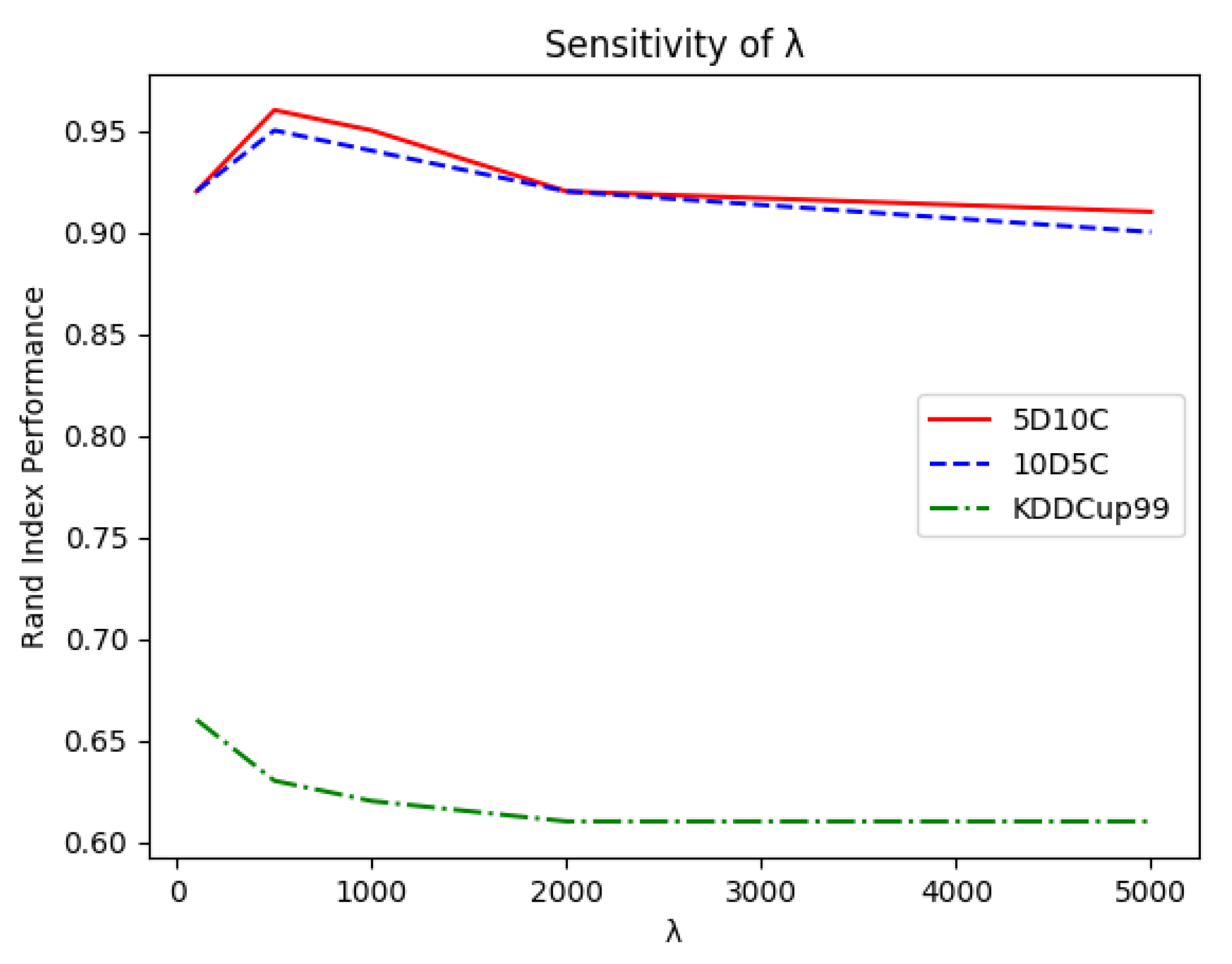
7.3. Sensitivity Analysis
Five parameters must be tuned before using OpStream for clustering dynamic data streams. In this section, the impact of each parameter on the classification performance is analysed in terms of the Rand index value.
To perform a thorough sensitivity analysis
the size of the landmark time window model was examined in the range ;
the value for the -neighbourhood method was examined within ;
the effect of the age threshold was examined by tuning in the interval ;
the WOA swarm sizes under analysis were obtained by adding 5 candidate solutions per experiment, from an initial value of 5 candidate solutions to a maximum of 30 candidate solutions;
the computational budget for the optimisation process, expressed in terms of “max iterations”number, was increased by 5 iterations per experiment starting with 5 up to a maximum of 30 iterations.
OpStream was run on three datasets for this sensitivity analysis, namely 5D10C, 10D5C and KDDC–99, and the results are graphically shown in the figures reported below.
Figure 4 shows that too high window sizes were not beneficial, and the best performances were obtained in the rage of
data points. In particular, a peak was obtained with a size of 1000 for the two artificially prepared datasets. Conversely, slightly inferior sizes might be preferred for the
KDDC–99 dataset. In general, there was no need to use more than 2000 data points, as the performance would remain constant or slightly deteriorate.
With reference to
Figure 5, it was evident that
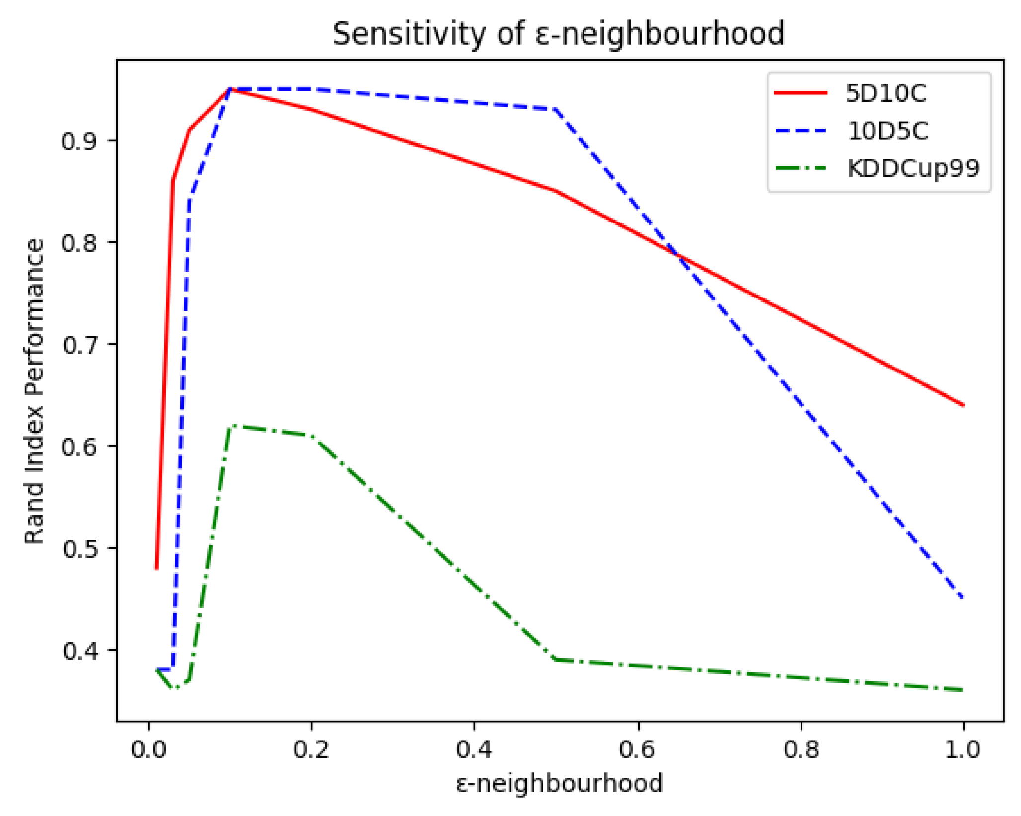
did not require fine tuning in a wide range as the best performances were obtained within
and then linearly decreased over the remaining admissible values. This can be easily explained as too low values would prevent microclusters from merging while too high values would force OpStream to merge dissimilar clusters. In both cases, the outcome would be a very poor classification. This observation facilitated the tuning process as it meant that it was worth trying values for
of
and
and perhaps one or two intermediary values.
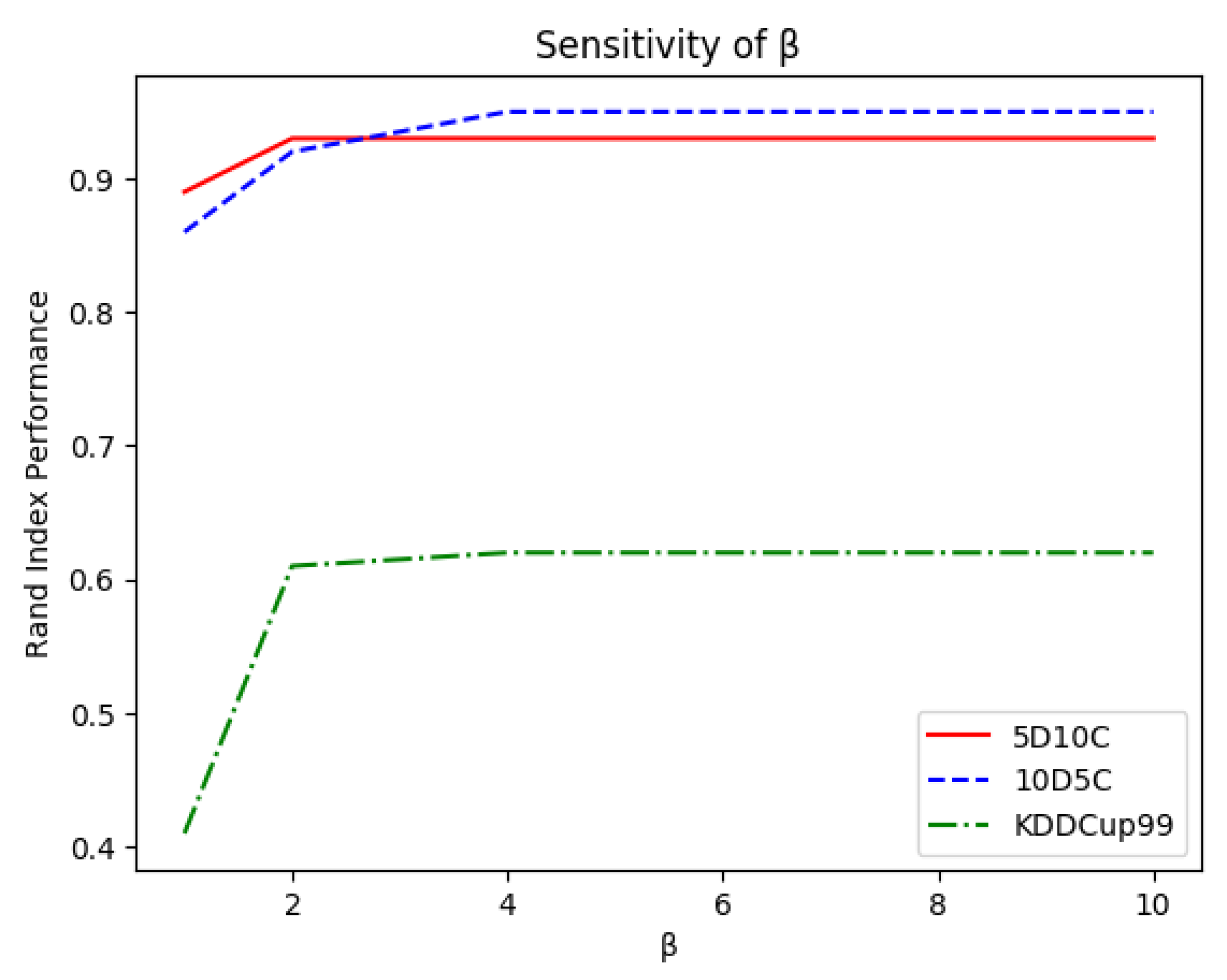
As for
, the curves in
Figure 6 show that OpStream was not sensitive to the value chosen for removing outdated clusters as long as
. This meant that clusters could be technically left in the buffers for a long time without affecting the performance of the classifier. From a more practical point of view, for memory issues, it was preferable to free buffers from unnecessary microclusters in a timely manner. A sensible choice is
, as too low values might prevent similar clusters from being merged due to the lack of time required for performing such a process.
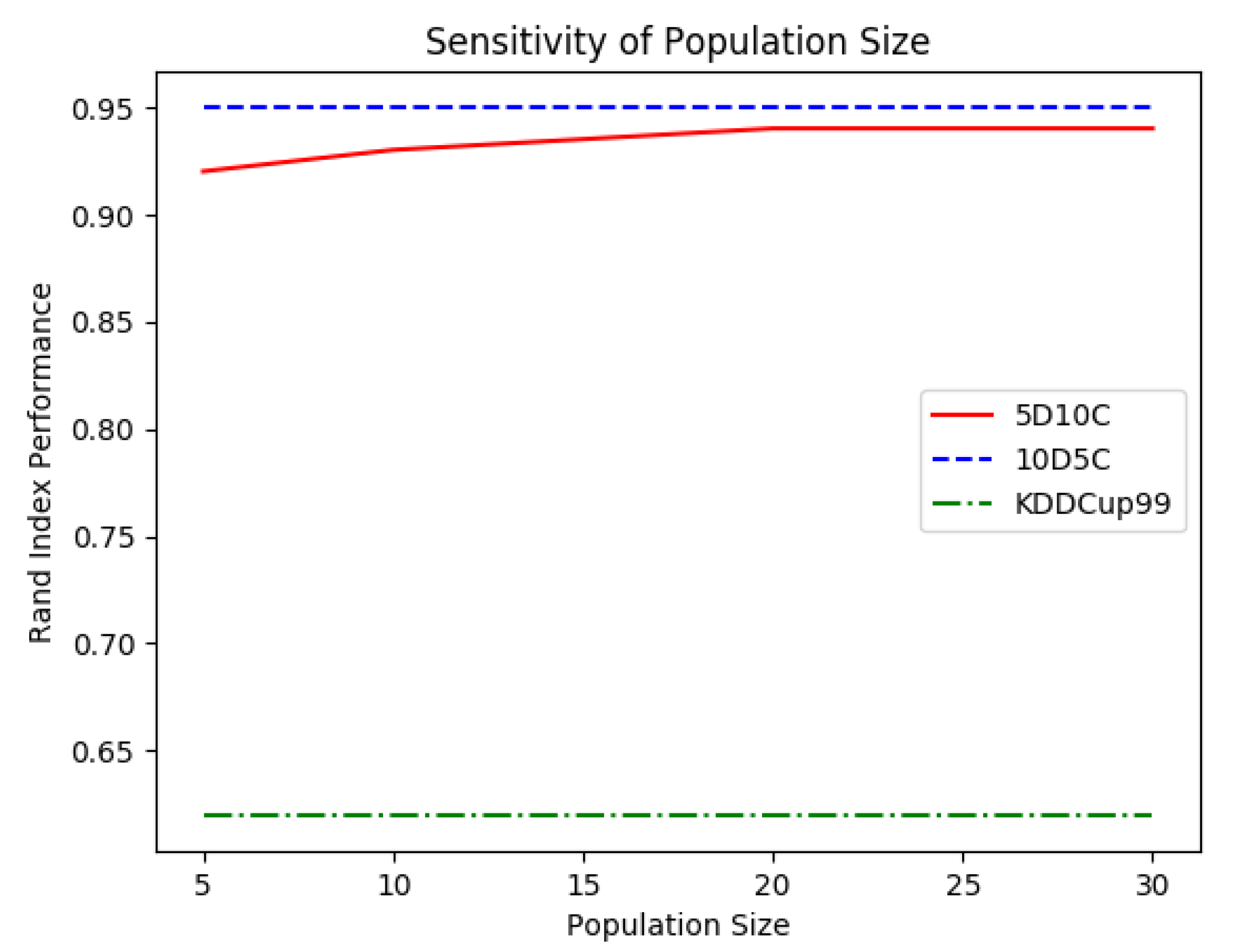
It can be noted that a small number of candidate solutions was used for the optimisation phase. This choice was made for multiple reasons. First, it has been recently shown that a high number of solutions can increase the structural biases of the algorithm [
52], which is not wanted as the algorithm has to be “general-purpose” to handle all possible scenarios obtained in the dynamic domain. Second, due to the time limitations related to the nature of this application domain, a high number of candidate solutions was to be avoided as it would slow down the converging process. This is not admissible in the real-time domain where also the computational budget is kept very low. Third, as shown in
Figure 7, the WOA method used in OpStream seemed to work efficiently regardless of the employed number of candidate solutions, as long as it was greater than 20.
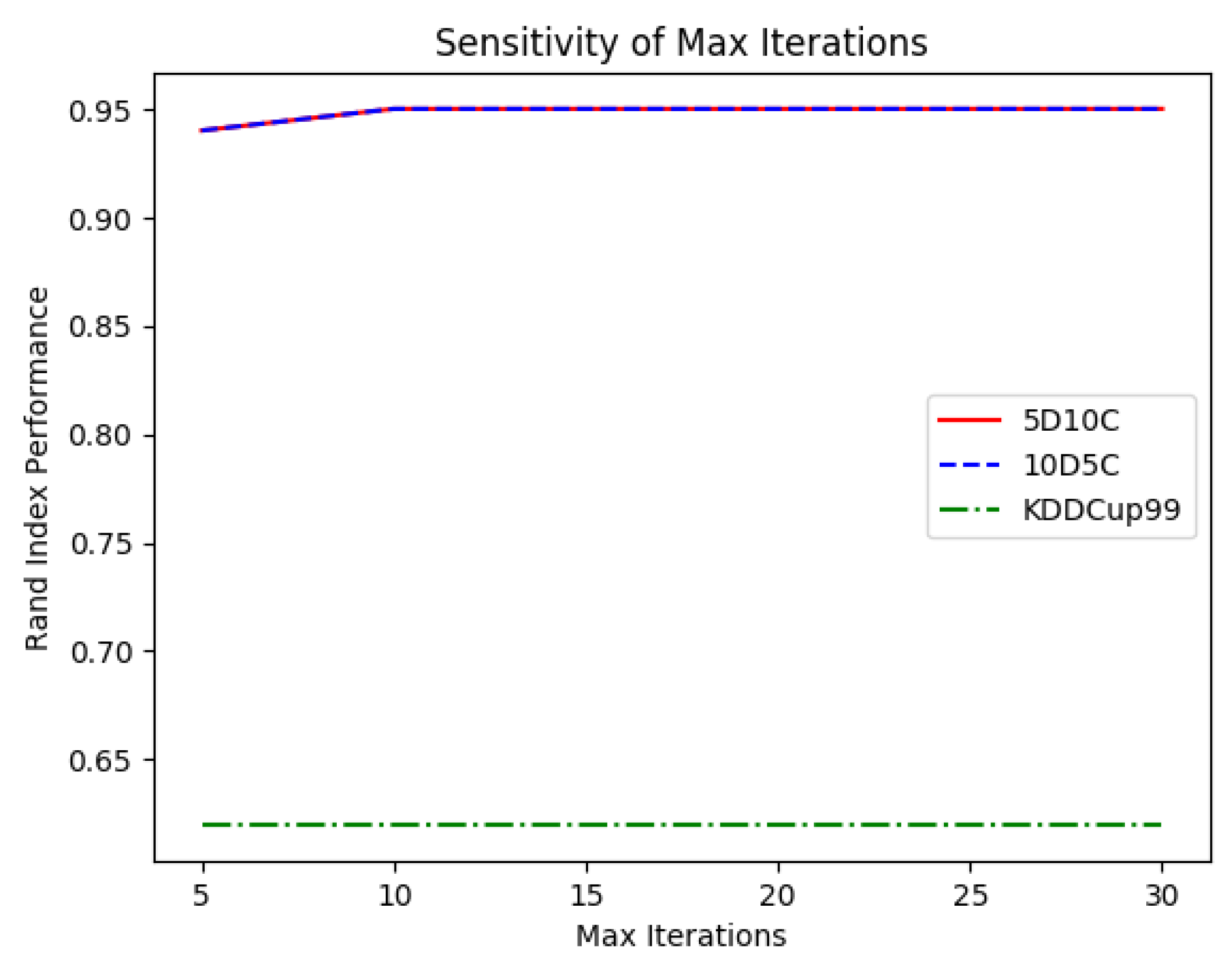
Similar conclusions can be made for the computational budget. According to
Figure 8, it was not necessary to prolong the duration of the WOA optimisation process for more than 10 iterations. This makes sense in dynamic domains, where the problem changes very frequently, thus making the exploitation phase less important.
7.4. Comparison with Past Studies on Intrusion Detection
One last comparison was performed to complete this study. This was performed on a specific application domain, i.e., network intrusion detection, by means of the “KDD–cup 99” database [
53]. The comparison algorithms employed in this work, i.e., DenStream and CluStream, were both tested on this dataset in their original papers [
18,
25], respectively. Despite the fact that OpStream is not meant for datasets with overlapping multi-density clusters, as in KDD–cup 99, we executed it over such a dataset to test its versatility. Results are displayed in
Table 7 where the last column indicates the average performance of the clustering method by computing:
Surprisingly, OpStream had an AVG better performance than CluStream, due to the fact that it significantly outperformed it in terms of F-measure and purity and displayed a state-of-the-art behaviour in terms of the purity value. As expected, DenStream provided the best performance, thus being preferable in this application domain unless a fast real-time response is required. In the latter case, its high computational cost could prevent DenStream from being successfully used [
18].
8. Conclusions and Future Work
Experimental numerical results showed that the proposed OpStream algorithm was a promising tool for clustering dynamic data streams as it was competitive and outperformed the state-of-the-art on several occasions. This approach could then be applied in several challenging application domains where satisfactory results are difficult to obtain with clustering methods. Thanks to its optimisation driven initialisation phase, OpStream displays high accuracy, robustness to noise in the dataset and versatility. In particular, we found out that its WOA implementation was efficient, scalable (both in term of dataset dimensionality and number of clusters) and resilient to parameters’ variations. Moreover, due to a low number of parameters to be tuned in WOA, this optimisation algorithm was preferred over other approaches returning similar accuracy values as DE and BAT. Finally, this study clearly showed that hybrid clustering methods are promising and more suitable than classic approaches to address challenging scenarios.
Possible improvements can be done to address some of the aspects arising during the experimental section. First, the deterioration of the performance over unevenly distributed datasets, as
KDDC-99, will be investigated. A simple solution to this problem is to embed non-density based clustering algorithms into the OpStream framework. Second, since the proposed methods do not benefit from preceding optimisation processes (as shown in
Figure 8), probably because of the dynamic nature of the problem, the optimisation algorithm employing “restart” mechanisms will be implemented and tested. These algorithms usually work on a very short computational budget and handle dynamic domains better than others by simply re-sampling the initial point where a local search routine is applied, as, e.g., [
54], or by also adding to it information from the previous past solution with the “inheritance” method [
55,
56,
57].
It is also worthwhile to extend OpStream to handle overlapping multi-density clusters in dynamic data streams, as these cases are not currently addressable and are common in some real-world scenarios, such as network intrusion detection [
51] and Landsat satellite image discovery [
58].


 ,
, 


