Abstract
A high-order compact (HOC) implicit difference scheme is proposed for solving three-dimensional (3D) unsteady reaction diffusion equations. To discretize the spatial second-order derivatives, the fourth-order compact difference operators are used, and the third- and fourth-order derivative terms, which appear in the truncation error term, are also discretized by the compact difference method. For the temporal discretization, the multistep backward Euler formula is used to obtain the fourth-order accuracy, which matches the spatial accuracy order. To accelerate the traditional relaxation methods, a multigrid method is employed, and the computational efficiency is greatly improved. Numerical experiments are carried out to validate the accuracy and efficiency of the present method.
1. Introduction
Reaction diffusion systems are widely used to describe the similar diffusion of all kinds of phenomena in modern science, such as the diffusion of gas, the infiltration of liquid concentration, gene diffusion in population, etc. Most of these systems contain nonlinear reaction terms, which make it difficult to obtain the exact solutions [1,2]. Therefore, it is most meaningful to investigate the accurate, efficient and stable numerical approaches of these systems.
In past decades, many researchers have been focusing on using efficient numerical methods for solving reaction diffusion equations. For instance, Madzvamuse and Maini [2] studied the implications of a mesh structure on the numerically computed solutions of a reaction diffusion model equation. Wang and Guo [3] proposed a spatially fourth-order and temporally second-order accuracy implicit finite difference monotone scheme for solving nonlinear reaction diffusion equations. Araújo et al. [4] proved the convergence properties of a class of implicit and semi-implicit finite difference schemes for solving nonlinear reaction diffusion equations. Zhu et al. [5] proposed Galerkin methods for solving the reaction diffusion system. Fernandes et al. [6] proposed an alternating direction implicit (ADI) method based on an extrapolated Crank‒Nicolson orthogonal spline collocation method. Gu et al. [7] proposed a high-order compact ADI difference scheme to solve a 3D reaction diffusion equation with Dirichlet boundary condition. Liao [8] extended the method to solve this 3D reaction diffusion equation with Neumann boundary condition.
Wang [9] proposed a higher-order compact ADI method and a monotonous iterative algorithm for solving the reaction diffusion equations. Tian [10] proposed a cubic spline difference scheme for solving the one-dimensional (1D) reaction diffusion equation. Hasnain et al. [11] used the fourth-order Douglas implicit scheme to solve the 3D reaction diffusion equation with nonlinear source term. Ge et al. [12] proposed a high-order compact (HOC) scheme and an adaptive method to solve the 1D nonlinear degenerate singular reaction diffusion equations.
There are also other high-order methods that have been developed to solve the reaction diffusion equation with the convection term. For instance, Kaya [13] developed two finite difference schemes with the Crank‒Nicolson method and backward Euler formula, respectively, for time discretization. Zhu and Rui [14] proposed an HOC difference scheme and an adaptive algorithm to solve a 1D convection diffusion reaction equation with nonlinear source terms. Iagar and Sánchez [15] proposed a method using the upper and lower solutions to study the existence and characteristics of blow up of the quasilinear reaction diffusion equation. Jiang and Zhang [16] proposed a method with arbitrary order of accuracy using the weighted essentially non-oscillatory approach. Jha and Singh [17] addressed the exponential basis and compact formulation when solving 3D convection diffusion reaction equations. Piquet et al. [18] presented a highly parallel finite difference method and a domain decomposition method and then applied them to solve the problems in computational fluid dynamics. Taken together, there are many references on nonlinear systems with source terms, and most of these methods can achieve fourth-order accuracy in spatial directions but only second-order accuracy in temporal direction. Therefore, it is still meaningful to identify a novel numerical method for solving the 3D nonlinear reaction diffusion equation.
This paper aims to develop an HOC difference scheme combined with the multigrid method to solve the 3D unsteady reaction diffusion equations; therefore, an unconditionally stable and high-order five-level fully implicit scheme is proposed. The main significances of this study are that the temporal accuracy of the developed scheme is able to reach the fourth-order and a multigrid method is used to accelerate the traditional iterative methods for solving the linear systems. The outline of this paper is as follows. In Section 2, the spatial derivative term is discretized by the fourth-order compact difference formula, and the time derivative term is discretized by the fourth-order backward Euler formula. For the calculation of the start-up levels, the first and second time levels are discretized using the Crank‒Nicolson method which is the second-order accuracy, and the third time level is discretized by the third-order backward Euler formula. In Section 3, a multigrid algorithm is designed to solve the linear systems. In Section 4, numerical experiments are conducted to validate the present method. In Section 5, a brief conclusion is given.
2. HOC Scheme for Unsteady Reaction Diffusion Equation
We consider the 3D unsteady reaction diffusion equation using Dirichlet boundary conditions. We will discuss how to design the fourth-order compact scheme for solving the 3D unsteady reaction diffusion equation in the following.
2.1. HOC Main Scheme
Consider the unsteady form of the following equations:
Assume that the problem domain is rectangular and and are constants. is the boundary and is the time interval. is the positive constant diffusion term coefficient, is the unknown function, is the nonlinear source function term, and are the smooth functions. We discretize the domain with uniform grids and split as meshes ; set to be the temporal grid step length and to be the spatial grid step length in the , and directions. The grid points are labeled as where and and
For the sake of simplicity, we use Figure 1 to denote the placement of the 19 points. We number the mesh points , , , , , , , , , , , , , , , , , and as , respectively.
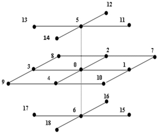
Figure 1.
Grid point stencil.
The details of the finite difference operators are given as follows:
The model Equation (1) can be rewritten as follows:
Using the Taylor series expansions at the grid point , we have
To keep the scheme compact, the fourth derivatives need to be discretized. We differentiate Equation (6) with ,, respectively as
Then, we substitute Equations (7)–(12) into Equation (6) to obtain the following difference equation:
We notice that
Omitting the truncation error term, we derive a compact difference scheme as the following:
To obtain an HOC scheme based on the mixed time derivatives in Equation (15), we only need to use the following second-order backward Euler formula [19] for discretization:
The following is the fourth-order backward Euler formula [19] for the time derivative in Equation (15):
Finally, substituting Equations (16) and (17) into Equation (15), neglecting the higher-order truncation error terms, and letting the mesh ratio be , the present HOC scheme can be rewritten as follows:
Equation (18) is the new HOC scheme we developed. It is easy to see from the derivation process that the truncation error of this scheme is , which means that the present HOC scheme has fourth-order accuracy in both time and space. It should be noted that only the spatial dimensions are compact in this scheme while the temporal dimension is not compact, since it involves five time levels. According to the conclusion in [19], the backward Euler formula is unconditionally stable when the accuracy is not higher than the sixth-order; therefore, we used the second-, third- and fourth-order backward Euler formulas in this paper; the HOC scheme is unconditionally stable.
2.2. HOC Schemes for the Start-Up Layers
We note that the scheme involves five time layers. In addition to knowing the initial value of the moment, it is necessary to obtain the values of the first, second and third time layers before we can move forward time. To ensure the accuracy of the schemes, we consider the value of Equation (18) at the moment using the Crank‒Nicolson method and Equations (16) and (17) are replaced by the following equation:
We simplify this equation to obtain
As seen from Equation (20), at time , the value of the first time layer can be solved; in addition, at time , the value of the second time level can be solved. The truncation error of this scheme is .
To obtain the value of the third time layer, for the mixed derivative term containing the time, the second-order backward Euler Formula (16) is adopted for discretization, and the third-order backward Euler formula can be used for the time derivative. Thus, Equation (17) is replaced by the following Equation [19]:
Letting , Equation (20) can be written as
The truncation error of this scheme is .
According to the above analysis, the HOC scheme is a fourth-order five-layer fully implicit scheme, and the scheme is unconditionally stable. That is, the HOC scheme in this paper can achieve fourth-order accuracy in both the spatial and temporal dimensions. For the HOC scheme, if we set , the first time and the second time layers keep an order of magnitude of ; the third time layer keeps an order of magnitude of ; and after the fourth time layer, the temporal dimension can achieve fourth-order accuracy. Therefore, the first three start-up layers have lower-order accuracy than the fourth-order accuracy. According to [19], the use of a second-order accuracy scheme to initialize a fourth-order accuracy scheme appears not to affect the overall order of accuracy because the cumulative error phase is relatively small due to the small number of advanced layers. The numerical experiments in Section 4 will also fully illustrate this point.
3. Multigrid Method
Various difference schemes are known to give rise to a number of linear algebraic equations, and thus, certain iterative methods are commonly used to solve them. However, the traditional iterative methods have been found to be inefficient due to their slow convergence speeds. For this reason, the multigrid method has been adopted as the primary solution to these problems. The convection diffusion equations [20,21] and Poisson equation [22] are just a couple of examples of the many that have been solved using this method. Wang and Ge [23] developed a fourth-order compact difference scheme and employed the multigrid method to solve the general 2D elliptic equations.
In general, the multigrid method can be regarded as one of the better nontraditional iterative methods used to address a wide range of partial differential equations [24], which is achieved by going through several specific loops and recursive algorithms, including the V-cycle, W-cycle, full multigrid V-cycle (FMV) and so on. The relaxation operator, restriction operator and interpolation operator are the three essential elements for establishing the multigrid method. The main characteristic of the multigrid method is that it uses different meshes. First, this method conducts “polishing” on the fine mesh level. Then, this method transfers the residual to the coarse mesh using the restriction operator, solves the residual equation on the coarse mesh, and finally returns the error correction result to the fine mesh level through the interpolation operator. According to the characteristics of the scheme in this paper, the full weighting restriction operator in [24] is used.
Then, we remove the four corner points in (23) to increase the impact of the center point to twice that of the original. It can be expressed as follows:
The bilinear interpolation operators also in [24] are as follows:
represents the restriction operator from level to level ,
represents the interpolation operator from level to level ,
represents the error residuals for the fine grid level, and
represents the error residuals for the adjacent coarse grid level.
Then, as far as the relaxation operator is concerned, we use the alternating direction line Gauss‒Seidel relaxations to remove the residuals on each coarse grid.
4. Numerical Experiments
The results of numerical experiments on the 3D unsteady semi-linear diffusion reaction equation problems are given in this section to demonstrate the performances of the present HOC schemes and the multigrid method. All of the model problems with Dirichlet boundary conditions have the exact solutions. At each time layer, when the L2-norm of the residual on the finest grids is lower than a tolerance , it is assumed that the calculation is convergent at this time layer and then proceeds to the calculation of the next time layer. The multigrid V cycles (Num), the CPU time in seconds, the maximum absolute errors (Error) and the convergence order (Order) for the different numbers of grids are given in the tables for all problems. The code is written in the Fortran 77 programming language using double precision arithmetic. The configuration of the computer is an Intel(R) core(TM) i7-7600 CPU with 4 GB of memory. The error, ratio of errors with two different grid sizes and the convergence order are computed using the following formulas:
where is the numerical solution, and is the exact solution. and represent different numbers of coarse and fine grids, and and are the maximum absolute errors estimated for the two numbers of grids of coarse grid and adjacent fine grid , respectively.
4.1. Problem 1
Consider the following 3D reaction diffusion problem:
where its exact solution is
The maximum absolute errors, the convergence order and the CPU time are calculated for and when the tolerance of residual is set to for the HOC scheme and the Crank‒Nicolson scheme, and the results are given in Table 1 and Table 2, respectively. The numerical results show that the Crank‒Nicolson scheme is convergent with only the second-order accuracy for the spatial variables, but the proposed HOC scheme can achieve fourth-order accuracy in the spatial dimension. The HOC scheme yields more accurate solutions than those of the Crank‒Nicolson scheme. Furthermore, we can also see the present HOC difference scheme is more cost-effective than the Crank‒Nicolson scheme for computing an approximate solution with a given accuracy; e.g., the maximum absolute error computed from the present HOC difference with is and cost CPU time 44.89 s, which is more accurate than the result computed using the Crank‒Nicolson scheme with and the CPU cost is 954.30 s. This result shows the superiority of the present high-order methods.

Table 1.
Maximum absolute error (Error), convergence order (Order) and CPU time at for Example 1.
Table 2.
Maximum absolute error (Error), convergence order (Order) and CPU time at for Example 1.
4.2. Problem 2
We consider the following 3D reaction diffusion problem:
where its exact solution is
For comparison purposes, we use the HOC scheme and the Crank‒Nicolson scheme to compute the numerical solutions of Problem 2, and set the tolerance of residual to be .
In Table 3 and Table 4, maximum absolute error, convergence order, and CPU time are given with and , respectively. It can be seen that the HOC scheme achieves fourth-order accuracy while the Crank‒Nicolson scheme achieves only second-order accuracy with different grids. Moreover, this result shows that the maximum absolute error of the HOC scheme is 1–2 orders of magnitude lower than that of the Crank‒Nicolson scheme. The advantages of the HOC scheme are more obvious when the number of grids increases. This result also shows that the present high-order scheme is more accurate.
Table 3.
Maximum absolute error (Error), convergence order (Order) and CPU time at for Example 2.
Table 4.
Maximum absolute error (Error), convergence order (Order) and CPU time at for Example 2.
4.3. Problem 3
Consider the following 3D reaction diffusion problem:
where its exact solution is
Problem 3 is the nonlinear unsteady reaction diffusion equation. We use the proposed HOC scheme and the scheme proposed in [6] to compute the numerical solution of Problem 3. The maximum absolute errors with different values of and at are listed in Table 5, and we set the tolerance of residual to be . We can clearly see that when , the maximum absolute errors of the present scheme and Gu et al.’s scheme [6] are almost identical. With the increase of the number of grids, the present scheme produces much better solutions. In Table 6, speed-up efficiency of the multigrid method is demonstrated. For comparisons, the traditional iterative method is also used to calculate the solution of this problem. All computed results are obtained with at . We can see that both the number of iterations and CPU time of the multigrid method are less than that of the traditional iterative method. These results show the superiority of the multigrid method.
Table 5.
Maximum absolute error (Error) and convergence order (Order) at for Example 3.
Table 6.
Speed-up efficiency of multigrid method compared to traditional method with for Example 3.
5. Conclusions
In this paper, a fully implicit five-layer high-order compact difference scheme is proposed for solving the 3D unsteady reaction diffusion equations. The truncation error of the main scheme is , which means that the overall accuracy of the HOC scheme achieves the fourth-order when . Although the accuracy order of the first three start-up layers is lower than the fourth, we numerically validate that it does not affect the overall accuracy of the present method. We also emphasize that the temporal accuracy of the present method in this paper is the fourth-order, which allows us to use a bigger time step length than the second-order schemes in the literature (see [3,7,10,12,14]). Consequently, the computational cost would be decreased because less time layers are needed for the present temporal high-order scheme than those temporal low-order schemes. The computational efficiency is improved when the multigrid acceleration technique is adopted in this paper. Numerical experiments are conducted to demonstrate the accuracy of the present scheme and the efficiency of the multigrid method. It is shown that the present HOC scheme is more accurate than those in the literature and the efficiency of the multigrid method is higher than the traditional iterative method. In addition, the HOC method can be directly extended to the numerical solutions of unsteady convection diffusion reaction equations, and unsteady incompressible Navier‒Stokes equations, such as the work of Méndez et al. work in [25], where the spectral element method is used.
Author Contributions
Methodology, L.W.; writing—review and editing, L.W.; conceptualization, X.F.; data curation, X.F.; investigation, L.W.; formal analysis, X.F.
Funding
Thanks to the National Natural Science Foundation of China (11772165 and 11701306). Thanks to the Foundation of Ningxia Normal University (NXSFZDA1803)
Acknowledgments
The authors are deeply indebted to the anonymous referees for their very careful reading and valuable comments and suggestions which immensely improved the previous version of our manuscript.
Conflicts of Interest
The authors declare no conflict of interest.
Nomenclature
| constants | the second- and fourth-order spatial derivatives in the directions, respectively | ||
| maximum absolute error | |||
| numbers of the multigrid V cycles | |||
| the CPU time in seconds | |||
| forcing function | the fourth-order spatial mixed derivatives | ||
| spatial second derivative of | |||
| spatial grid step length | the second-order spatial derivatives of | ||
| index of grid point in directions, respectively | |||
| time level | |||
| numbers of grids for space and time | the first- and the second-order temporal derivatives of | ||
| numbers of grids of coarse and fine meshes, respectively | |||
| convergence order | spatial coordinate in the directions | ||
| interpolation operator from level to level | |||
| mesh ratio | spatial discrete points | ||
| the error ratio of different grids | Greek symbols | ||
| residuals for coarse grid levels | the first- and the second-order central different operators | ||
| residuals for fine grid levels | |||
| restriction operator from level to | positive constant diffusion term coefficient | ||
| Max | maximum value function | ||
| time coordinate | boundary conditions | ||
| total time | initial conditions | ||
| solution of Equation (18) | temporal grid step length | ||
| exact solution at grid point | computational domain | ||
| numerical solution at grid point | domain boundary | ||
References
- Ames, W.F. Nonlinear Partial Differential Equations in Engineering; Academic Press: New York, NY, USA, 1965. [Google Scholar]
- Madzvamuse, A.; Maini, P.K. Velocity-induced numerical solutions of reaction-diffusion systems on continuously growing domains. J. Comput. Phys. 2007, 225, 100–119. [Google Scholar] [CrossRef]
- Wang, Y.; Guo, B. A monotone compact implicit scheme for nonlinear reaction-diffusion equations. J. Comp. Math. 2008, 26, 123–148. [Google Scholar]
- Araújo, A.; Barbeiro, S.; Serranho, P. Convergence of finite difference schemes for nonlinear complex reaction-diffusion processes. SIAM J. Numer. Anal. 2015, 53, 228–250. [Google Scholar] [CrossRef]
- Zhu, J.; Zhang, Y.T.; Newman, S.A.; Alber, M. Application of discontinuous galerkin methods for reaction-diffusion systems in developmental biology. J. Sci. Comput. 2009, 40, 391–418. [Google Scholar] [CrossRef]
- Fernandes, R.I.; Bialecki, B.; Fairweather, G. An ADI extrapolated Crank-Nicolson orthogonal spline collocation method for nonlinear reaction-diffusion systems on evolving domains. J. Comput. Phys. 2015, 299, 561–580. [Google Scholar] [CrossRef]
- Gu, Y.; Liao, W.; Zhu, J. An efficient high-order algorithm for solving systems of 3-D reaction-diffusion equations. J. Comput. Appl. Math. 2003, 155, 1–17. [Google Scholar] [CrossRef]
- Liao, W. A high-order ADI finite difference scheme for a 3D reaction-diffusion equation with neumann boundary condition. Numer. Methods Part. Differ. Equ. 2013, 29, 778–798. [Google Scholar] [CrossRef]
- Wang, Y.M.; Wang, J. A higher-order compact ADI method with monotone iterative procedure for systems of reaction–diffusion equations. Comput. Math. Appl. 2011, 62, 2434–2451. [Google Scholar] [CrossRef]
- Tian, Z. Cubic-spline difference schemes of high-order accuracy for diffusion reaction equation. J. Hubei Univ. 1997, 19, 111–115. (In Chinese) [Google Scholar]
- Hasnain, S.; Saqib, M.; Mashat, D.S. Fourth order Douglas implicit scheme for solving three dimension reaction diffusion equation with non-linear source term. AIP Adv. 2017, 7, 075011. [Google Scholar] [CrossRef]
- Ge, Y.; Cai, Z.; Sheng, Q. A compact adaptive approach for degenerate singular reaction-diffusion equations. Numer. Methods Part. Differ. Equ. 2018, 34, 1166–1187. [Google Scholar] [CrossRef]
- Kaya, A. Finite difference approximations of multidimensional unsteady convection-diffusion-reaction equations. J. Comput. Phys. 2015, 285, 331–349. [Google Scholar] [CrossRef]
- Zhu, X.; Rui, H. High-order compact difference scheme of 1D nonlinear degenerate convection-reaction-diffusion equation with adaptive algorithm. Numer. Heat Transf. Part B Fundam. 2019, 75, 43–46. [Google Scholar] [CrossRef]
- Iagar, R.G.; Sánchez, A. Blow up profiles for a quasilinear reaction-diffusion equation with weighted reaction with linear growth. J. Dyn. Differ. Equ. 2019, 31, 2061–2094. [Google Scholar] [CrossRef]
- Jiang, T.; Zhang, Y.T. Krylov single-step implicit integration factor WENO methods for advection-diffusion-reaction equations. J. Comput. Phys. 2016, 311, 22–44. [Google Scholar] [CrossRef]
- Jha, N.; Singh, B. Exponential basis and exponential expanding grids third (fourth)-order compact schemes for nonlinear three-dimensional convection-diffusion-reaction equation. Adv. Differ. Equ. 2019, 2019, 339. [Google Scholar] [CrossRef]
- Piquet, A.; Zebiri, B.; Hadjadj, A.; Shadloo, M.S. A parallel high-order compressible flows solver with a domain decomposition method in the generalized curvilinear coordinates system. Int. J. Numer. Methods Heat Fluid Flow 2019. [Google Scholar] [CrossRef]
- Strikwerda, J.C. High order accurate schemes for incompressible viscous flow. Int. J. Numer. Meth. Fluids 1997, 24, 715–734. [Google Scholar] [CrossRef]
- Gupta, M.M.; Zhang, J. High accuracy multigrid solution of the 3D convection-diffusion equation. Appl. Math. Comput. 2000, 113, 249–274. [Google Scholar] [CrossRef]
- Ge, Y.; Cao, F. Multigrid method based on the transformation-free HOC scheme on nonuniform grids for 2D convection diffusion problems. J. Comput. Phys. 2011, 230, 4051–4070. [Google Scholar] [CrossRef]
- Ge, Y.; Cao, F.; Zhang, J. A transformation-free HOC scheme and multigrid method for solving the 3D Poisson equation on nonuniform grids. J. Comput. Phys. 2013, 234, 199–216. [Google Scholar] [CrossRef]
- Wang, Y.; Ge, Y. High-order compact difference scheme and multigrid method for solving the 2D elliptic problems. Math. Probl. Eng. 2018. [Google Scholar] [CrossRef]
- Wesseling, P.W. An Introduction to Multigrid Methods; Wiley: Chichester, UK, 1992. [Google Scholar]
- Méndez, M.; Shadloo, M.S.; Hadjadj, A.; Ducoin, A. Boundary layer transition over a concave surface caused by centrifugal instabilities. Comput. Fluids 2018, 171, 135–153. [Google Scholar] [CrossRef]
© 2019 by the authors. Licensee MDPI, Basel, Switzerland. This article is an open access article distributed under the terms and conditions of the Creative Commons Attribution (CC BY) license (http://creativecommons.org/licenses/by/4.0/).