Generalized High-Order Classes for Solving Nonlinear Systems and Their Applications

Abstract

A generalized high-order class for approximating the solution of nonlinear systems of equations is introduced. First, from a fourth-order iterative family for solving nonlinear equations, we propose an extension to nonlinear systems of equations holding the same order of convergence but replacing the Jacobian by a divided difference in the weight functions for systems. The proposed GH family of methods is designed from this fourth-order family using both the composition and the weight functions technique. The resulting family has order of convergence 9. The performance of a particular iterative method of both families is analyzed for solving different test systems and also for the Fisher’s problem, showing the good performance of the new methods.

1. Introduction

During the last few decades, there has been a wide amount of interest in designing iterative schemes for estimating both equations and systems of equations presenting nonlinearities. Since the problems of finding a zero $x^{*}\in D$ of a system of nonlinear equations $F\left(x\right)=0$, where $F:D\subseteq {\mathbb{R}}^n⟶{\mathbb{R}}^n$, are present in science and engineering, the iterative methods are an ideal candidate for finding the solutions.

There is extensive literature on iterative methods for solving nonlinear equations, good overviews can be found in [1,2]. However, the extension of schemes from equations to systems of equations is not always trivial. Based on the Kung–Traub’s conjecture for nonlinear equations [3], several optimal methods of three steps can be found in the recent works [4,5]. There are other interesting methods on the research that reach higher order of convergence [6].

In this paper, we present a new family of iterative methods for solving nonlinear systems of equations with convergence order nine. This class, named GH family, has two weight functions and four steps on its iterative expression. It needs one evaluation of the Jacobian matrix and four functional evaluations of the nonlinear function per iteration. Previously, a fourth-order family with only a weight function is proposed. This family is the basis for designing the iterative schemes of the GH family with a composition-type technique. The development of the family covers Section 2. In order to check the feasibility of the proposed schemes to solve nonlinear systems of equations, Section 3 shows the numerical results when the fourth-order scheme is used for solving Fisher’s partial differential equation and when the ninth-order family is applied to several test functions. Finally, Section 4 collects the main conclusions of the work.

Some basic definitions must be recalled for analyzing the order of convergence of the methods. Further details can be found in [4,7] and also the notation used in this work.

2. The GH Family for Solving Systems of Nonlinear Equations

In [8], a new family of iterative methods for solving nonlinear equations is introduced. Its iterative expression is

$$\begin{array}{ccc}\hfill y_k& =& x_k-{\displaystyle \frac{f\left(x_k\right)}{f^{\prime }\left(x_k\right)}},\hfill \\ \hfill x_{k+1}& =& x_k-G\left({\eta }_k\right){\displaystyle \frac{f\left(x_k\right)}{f^{\prime }\left(x_k\right)}},k=0,1,2,\dots ,\hfill \end{array}$$

(1)

where $G\left({\eta }_k\right)$ is a weight function with ${\eta }_k=\frac{f\left(y_k\right)}{f\left(x_k\right)}$. Its order of convergence is analyzed in the following result. A complete proof can be found in [8]. Our purpose in this paper is to extend this result for the case of multidimensional problems.

Theorem 1.

Let $f:\mathsf{\Omega }\subset \mathbb{R}⟶\mathbb{R}$ be a real sufficiently differentiable function in an open interval Ω and let $x^{*}\in \mathsf{\Omega }$ be a simple root of $f\left(x\right)=0$. If $x_0$ is close enough to $x^{*}$ and $G\left(\eta \right)$ satisfies conditions $G\left(0\right)=G^{\prime }\left(0\right)=1$ and $G^{″}\left(0\right)=4$, then all the iterative methods of family (1) converge to $x^{*}$ with fourth-order of convergence, their error equation being

$$e_{k+1}=(5c_2^3-c_2{c}_3)e_k^4+\mathcal{O}\left(e_k^5\right),$$

(2)

where $e_k=x_k-x^{*}$ and $c_j=\frac{f^{\left(j\right)}\left(x^{*}\right)}{j!f^{\prime }\left(x^{*}\right)}$, $j\ge 2$.

In order to extend family (1) for solving nonlinear systems, an alternative definition for variable ${\eta }_k$ is required. For this purpose, we develop the expression as follows:

$$\begin{array}{c}\hfill {\eta }_k=\frac{f\left(y_k\right)}{f\left(x_k\right)}=\frac{f\left(y_k\right)}{(x_k-y_k)f^{\prime }\left(x_k\right)}=-\frac{f[y_k,x_k]}{f^{\prime }\left(x_k\right)}+\frac{f\left(x_k\right)}{(x_k-y_k)f^{\prime }\left(x_k\right)}=\frac{f^{\prime }\left(x_k\right)-f[y_k,x_k]}{f^{\prime }\left(x_k\right)}.\end{array}$$

So, the extension of family (1) for solving systems of nonlinear equations turns into

$$\begin{array}{ccc}\hfill y^{\left(k\right)}& =& x^{\left(k\right)}-{\left[F^{\prime }\left(x^{\left(k\right)}\right)\right]}^{-1}F\left(x^{\left(k\right)}\right),\hfill \\ \hfill x^{(k+1)}& =& x^{\left(k\right)}-G\left({\eta }_k\right){\left[F^{\prime }\left(x^{\left(k\right)}\right)\right]}^{-1}F\left(x^{\left(k\right)}\right),\hfill \end{array}$$

(3)

where

$${\eta }_k={\left[F^{\prime }\left(x^{\left(k\right)}\right)\right]}^{-1}(F^{\prime }\left(x^{\left(k\right)}\right)-[y^{\left(k\right)},x^{\left(k\right)};F])$$

(4)

and $G:{\mathbb{R}}^{n\times n}⟶{\mathbb{R}}^{n\times n}$ is a matrix weight function. Furthermore, if $X={\mathbb{R}}^{n\times n}$ denotes the space of all $n\times n$ real matrices, then we can define (see [9]) $G:X⟶X$ such that its Fréchet derivatives satisfy:

(a)

$G^{\prime }\left(u\right)\left(v\right)=G_{1}uv$, being $G^{\prime }:X⟶\mathcal{L}\left(X\right)$, $G_1\in \mathbb{R}$, and $\mathcal{L}\left(x\right)$ denotes the space of linear mappings from X to itself,

(b)

$G^{″}(u,v)\left(w\right)=G_{2}uvw$, where $G^{″}:X\times X⟶\mathcal{L}\left(X\right)$ and $G_2\in \mathbb{R}$.

(c)

$G^{‴}(u,v,w)\left(t\right)=G_{3}uvwt$, for $G^{‴}:X\times X\times X⟶\mathcal{L}\left(X\right)$ and $G_3\in \mathbb{R}$.

Moreover, the definition of ${\eta }_k$ in Label (4) uses the divided difference operator of F on ${\mathbb{R}}^n$, $[·,·;F]:\mathsf{\Omega }\times \mathsf{\Omega }\subset {\mathbb{R}}^n\times {\mathbb{R}}^n⟶\mathcal{L}\left({\mathbb{R}}^n\right)$, defined in [10] as

$$[x,y;F](x-y)=F\left(x\right)-F\left(y\right),\mathrm{for}\mathrm{any}x,y\in \mathsf{\Omega }.$$

The next result shows the order of convergence of family (3).

Theorem 2.

Let the nonlinear function $F:\mathsf{\Omega }\subseteq {\mathbb{R}}^n⟶{\mathbb{R}}^n$ be a sufficiently Fréchet differentiable in an open convex set Ω, $x^{*}\in \mathsf{\Omega }$ a solution of the system $F\left(x\right)=0$. It must be also satisfied that $F^{\prime }\left(x\right)$ is continuous and nonsingular in $x^{*}$. Let us suppose that the initial guess $x^{\left(0\right)}\in {\mathbb{R}}^n$ is close enough to $x^{*}$ and $G\left({\eta }_k\right)$ satisfies $G\left(0\right)=I$, $G_1=1$, $G_2=4$ and $|G_3|<+\infty$, where I denotes the identity matrix of size $n\times n$. Then, family (3) converges to $x^{*}$ with order of convergence 4, its error equation being

$$e^{(k+1)}=\left(-C_3{C}_2+\left(5-{\displaystyle \frac{1}{6}}{G}_3\right)C_2^3\right)e^{{\left(k\right)}^4}+\mathcal{O}\left(e^{{\left(k\right)}^5}\right),$$

$e^{\left(k\right)}=x^{\left(k\right)}-x^{*}$ being the error in the kth iteration and $C_j={\displaystyle \frac{1}{j!}}{\left[F^{\prime }\left(x^{*}\right)\right]}^{-1}{F}^{\left(j\right)}\left(x^{*}\right)$, $j\ge 2$.

Proof. 

Let us denote by $e^{\left(k\right)}=x^{\left(k\right)}-x^{*}$ for all k the error in iteration k. By using Taylor series expansions around $x^{*}$, $F\left(x^{\left(k\right)}\right)$ and $F^{\prime }\left(x^{\left(k\right)}\right)$ can be expressed as

$$\begin{array}{ccc}\hfill F\left(x^{\left(k\right)}\right)& =& F^{\prime }\left(x^{*}\right)\left[e^{\left(k\right)}+C_2{e}^{{\left(k\right)}^2}+C_3{e}^{{\left(k\right)}^3}+C_4{e}^{{\left(k\right)}^4}\right]+\mathcal{O}\left(e^{{\left(k\right)}^5}\right),\hfill \\ \hfill \\ \hfill F^{\prime }\left(x^{\left(k\right)}\right)& =& F^{\prime }\left(x^{*}\right)\left[I+2C_2{e}^{\left(k\right)}+3C_3{e}^{{\left(k\right)}^2}+4C_4{e}^{{\left(k\right)}^3}\right]+\mathcal{O}\left(e^{{\left(k\right)}^4}\right),\hfill \end{array}$$

(5)

where $C_j={\displaystyle \frac{1}{j!}}{\left[F^{\prime }\left(x^{*}\right)\right]}^{-1}{F}^{\left(j\right)}\left(x^{*}\right)$, $j\ge 2$. In the same way, it holds that

$${\left[F^{\prime }\left(x^{\left(k\right)}\right)\right]}^{-1}=\left[X_1+X_2{e}^{\left(k\right)}+X_3{e}^{{\left(k\right)}^2}+X_4{e}^{{\left(k\right)}^3}\right]{\left[F^{\prime }\left(x^{*}\right)\right]}^{-1}+\mathcal{O}\left(e^{{\left(k\right)}^4}\right).$$

(6)

As ${\left[F^{\prime }\left(x^{\left(k\right)}\right)\right]}^{-1}{F}^{\prime }\left(x^{\left(k\right)}\right)=I$, we have $X_1=I$ and

$$X_j=-\sum _{i=2}^{j}i{X}_{j-i+1}{C}_i,j>1.$$

(7)

From (5) and (6), we have

$${\left[F^{\prime }\left(x^{\left(k\right)}\right)\right]}^{-1}F\left(x^{\left(k\right)}\right)=e^{\left(k\right)}-C_2{e}^{{\left(k\right)}^2}+J_3{e}^{{\left(k\right)}^3}+J_4{e}^{{\left(k\right)}^4}+\mathcal{O}\left(e^{{\left(k\right)}^5}\right)$$

(8)

for the values

$$J_j=C_j+\sum _{i=3}^j{X}_{j-i+2}{C}_{i-1}+X_j,j>2.$$

(9)

Now, from the above developments,

$$\begin{array}{c}\hfill y^{\left(k\right)}-x^{*}=e^{\left(k\right)}-{\left[F^{\prime }\left(x^{\left(k\right)}\right)\right]}^{-1}F\left(x^{\left(k\right)}\right)=C_2{e}^{{\left(k\right)}^2}-J_3{e}^{{\left(k\right)}^3}-J_4{e}^{{\left(k\right)}^4}+\mathcal{O}\left(e^{{\left(k\right)}^5}\right).\end{array}$$

The divided difference operator is defined by the formula of Gennochi–Hermite [10]

$$\left[x+h,x;F\right]={\int }_0^1{F}^{\prime }(x+th)dt,\forall x\in {\mathbb{R}}^n.$$

Expanding $F^{\prime }(x+th)$ in Taylor series around x and integrating, we have

$$\begin{array}{c}\hfill \left[x+h,x;F\right]=F^{\prime }\left(x\right)+\frac{1}{2}{F}^{″}\left(x\right)h+\frac{1}{6}{F}^{‴}\left(x\right)h^2+\mathcal{O}\left(h^3\right).\end{array}$$

In particular, for $y^{\left(k\right)}$ given by the first step of the family (3),

$$\begin{array}{ccc}\left[y^{\left(k\right)},x^{\left(k\right)};F\right]& =& \sum _{i=1}^3\frac{1}{i!}{F}^{\left(i\right)}\left(x^{\left(k\right)}\right){\left(y^{\left(k\right)}-x^{\left(k\right)}\right)}^{i-1}+\mathcal{O}\left(e^{{\left(k\right)}^4}\right)\hfill \\ & =& F^{\prime }\left(x^{*}\right)[I+C_2{e}^{\left(k\right)}+S_2{e}^{{\left(k\right)}^2}+S_3{e}^{{\left(k\right)}^3}]+\mathcal{O}\left(e^{{\left(k\right)}^4}\right)\end{array}$$

(10)

is obtained, where $S_i$, $i\ge 2$, is

$$\begin{array}{cc}\hfill S_2& =C_2^2+C_3,\hfill \\ \hfill S_3& =C_4+C_3{C}_2-C_2{J}_3.\hfill \end{array}$$

(11)

Now, the value of ${\eta }_k$ is given by:

$$\begin{array}{c}\hfill {\eta }_k={\left[F^{\prime }\left(x^{\left(k\right)}\right)\right]}^{-1}\left(F^{\prime }\left(x^{\left(k\right)}\right)-[y^{\left(k\right)},x^{\left(k\right)};F]\right)=C_2{e}^{\left(k\right)}+A_2{e}^{{\left(k\right)}^2}+A_3{e}^{{\left(k\right)}^3}+\mathcal{O}\left(e^{{\left(k\right)}^4}\right),\end{array}$$

where

$$\begin{array}{cc}\hfill A_2& =2C_3-3C_2^2,\hfill \\ \hfill A_3& =8C_2^3+3C_4-6C_2{C}_3-4C_3{C}_2.\hfill \end{array}$$

(12)

By using (12), its successive powers are obtained:

$$\begin{array}{c}\hfill {\eta }_k^2=C_2^2{e}^{{\left(k\right)}^2}+B_3{e}^{{\left(k\right)}^3}+\mathcal{O}\left(e^{{\left(k\right)}^4}\right),\end{array}$$

where $B_3=C_2{A}_2+A_2{C}_2$, and

$$\begin{array}{c}\hfill {\eta }_k^3=C_2^3{e}^{{\left(k\right)}^3}+\mathcal{O}\left(e^{{\left(k\right)}^4}\right).\end{array}$$

Using the Taylor expansion of $G\left({\eta }_k\right)$ around 0, we get

$$\begin{array}{cc}\hfill G\left({\eta }_k\right)& =G\left(0\right)+G_1{\eta }_k+\frac{1}{2!}{G}_2{\eta }_k^2+\frac{1}{3!}{G}_3{\eta }_k^3+\mathcal{O}\left({\eta }_k^4\right)\hfill \\ \hfill & =G\left(0\right)+G_1{C}_2{e}^{\left(k\right)}+\left(G_1{A}_2+\frac{1}{2}{G}_2{C}_2^2\right)e^{{\left(k\right)}^2}+\left(G_1{A}_3+\frac{1}{2}{G}_2{B}_3+\frac{1}{6}{G}_3{C}_2^3\right)e^{{\left(k\right)}^3}+\mathcal{O}\left(e^{{\left(k\right)}^4}\right).\hfill \end{array}$$

Then,

$$\begin{array}{cc}G\left({\eta }_k\right){\left[F^{\prime }\left(x^{\left(k\right)}\right)\right]}^{-1}F\left(x^{\left(k\right)}\right)& =G\left(0\right)e^{\left(k\right)}+(G_1-G\left(0\right))C_2{e}^{{\left(k\right)}^2}\\ & +\left(G\left(0\right)J_3+G_1(-C_2^2+A_2)+\frac{1}{2}{G}_2{C}_2^2\right)e^{{\left(k\right)}^3}\hfill \\ & +(G\left(0\right)J_4+G_1(C_2{J}_3-A_2{C}_2+A_3)\hfill \\ & +\frac{1}{2}{G}_2(-C_2^3+B_3)+\frac{1}{6}{G}_3{C}_2^3)e^{{\left(k\right)}^4}+\mathcal{O}\left(e^{{\left(k\right)}^5}\right).\hfill \end{array}$$

Finally, the error equation of family (3) is

$$\begin{array}{ccc}{e}^{(k+1)}& =& e^{\left(k\right)}-G\left({\eta }_k\right){\left[F^{\prime }\left(x^{\left(k\right)}\right)\right]}^{-1}F\left(x^{\left(k\right)}\right)\hfill \\ & =& (I-G\left(0\right))e^{\left(k\right)}+(G\left(0\right)-G_1)C_2{e}^{{\left(k\right)}^2}+\left(-G\left(0\right)J_3+G_1(C_2^2-A_2)-\frac{1}{2}{G}_2{C}_2^2\right)e^{{\left(k\right)}^3}\\ & & +\left(-G\left(0\right)J_4+G_1(-C_2{J}_3+A_2{C}_2-A_3)+\frac{1}{2}{G}_2(C_2^3-B_3)\frac{1}{6}{G}_3{C}_2^3\right)e^{{\left(k\right)}^4}+\mathcal{O}\left(e^{{\left(k\right)}^5}\right).\end{array}$$

By applying conditions $G\left(0\right)=I$, $G_1=1$ and $G_2=4$, the error equation turns into

$$e^{(k+1)}=\left(-C_3{C}_2+\left(5-\frac{1}{6}{G}_3\right)C_2^3\right)e^{{\left(k\right)}^4}+\mathcal{O}\left(e^{{\left(k\right)}^5}\right),$$

so the iterative family (3) is fourth-order convergent. □

Trying to design a higher-order class with the same structure, we now consider the fourth-step iterative family:

$$\begin{array}{ccc}\hfill y^{\left(k\right)}& =& x^{\left(k\right)}-{\left[F^{\prime }\left(x^{\left(k\right)}\right)\right]}^{-1}F\left(x^{\left(k\right)}\right),\hfill \\ \hfill z^{\left(k\right)}& =& x^{\left(k\right)}-G\left({\eta }_k\right){\left[F^{\prime }\left(x^{\left(k\right)}\right)\right]}^{-1}F\left(x^{\left(k\right)}\right),\hfill \\ \hfill w^{\left(k\right)}& =& z^{\left(k\right)}-[F^{\prime }{\left(x^{\left(k\right)}\right]}^{-1}F\left(z^{\left(k\right)}\right),\hfill \\ \hfill x^{(k+1)}& =& z^{\left(k\right)}-H\left({\tau }_k\right){\left[F^{\prime }\left(x^{\left(k\right)}\right)\right]}^{-1}F\left(z^{\left(k\right)}\right),\hfill \end{array}$$

(13)

where $G\left({\eta }_k\right)$ and $H\left({\tau }_k\right)$ are two matrix weight functions with variables defined by

$$\begin{array}{ccc}\hfill {\eta }_k& =& {\left[F^{\prime }\left(x^{\left(k\right)}\right)\right]}^{-1}(F^{\prime }\left(x^{\left(k\right)}\right)-[y^{\left(k\right)},x^{\left(k\right)};F]),\hfill \\ \hfill {\tau }_k& =& {\left[F^{\prime }\left(x^{\left(k\right)}\right)\right]}^{-1}(F^{\prime }\left(x^{\left(k\right)}\right)-[z^{\left(k\right)},w^{\left(k\right)};F]).\hfill \end{array}$$

Let us recall that the iterative scheme (13), from now on called GH family, has been obtained by a composition-type of the iterative family (3) with itself. The convergence of GH family is analyzed in the next result.

Theorem 3.

Let the nonlinear function $F:\mathsf{\Omega }\subseteq {\mathbb{R}}^n⟶{\mathbb{R}}^n$ be a sufficiently Fréchet differentiable in an open convex set Ω, $x^{*}\in \mathsf{\Omega }$ a solution of the system $F\left(x\right)=0$. It must be also satisfied that $F^{\prime }\left(x\right)$ is continuous and nonsingular in $x^{*}$. Let us suppose that the initial estimation $x^{\left(0\right)}\in {\mathbb{R}}^n$ is close enough to $x^{*}$ and the weight functions $G\left({\eta }_k\right)$ and $H\left({\tau }_k\right)$ satisfy:

(i) 

$G\left(0\right)=I$, $G_1=1$, $G_2=4$ and $G_3=30$.

(ii) 

$H\left(0\right)=I$, $H_1=1$, $H_2=2$ and $H_3=6$.

Then, all the iterative methods of family (13) converge to $x^{*}$ with order of convergence 9.

Proof. 

By using the developments in the proof of Theorem 2 (with more terms in the error expressions) and also the same way to proceed, we obtain for the second step of family (13)

$$\begin{array}{cc}\hfill z^{\left(k\right)}-x^{*}& =e^{\left(k\right)}-G\left({\eta }_k\right){\left[F^{\prime }\left(x^{\left(k\right)}\right)\right]}^{-1}F\left(x^{\left(k\right)}\right)\hfill \\ \hfill & =-K_4{e}^{{\left(k\right)}^4}-K_5{e}^{{\left(k\right)}^5}-K_6{e}^{{\left(k\right)}^6}-K_7{e}^{{\left(k\right)}^7}-K_8{e}^{{\left(k\right)}^8}-K_9{e}^{{\left(k\right)}^9}+\mathcal{O}\left(e^{{\left(k\right)}^{10}}\right).\hfill \end{array}$$

(14)

The coefficients $K_j$ are obtained using expressions (7), (9), (11), and (12), and

$$\begin{array}{cc}\hfill S_4& =C_5+C_3{C}_2^2+C_4{C}_2-C_2{J}_4-C_3{J}_3,\hfill \\ \hfill S_5& =C_6+C_4{C}_2^2+C_5{C}_2-C_2{J}_5-C_3{J}_4-C_4{J}_3-C_3{C}_2{J}_3-C_3{J}_3{C}_2,\hfill \\ \hfill S_6& =C_7+C_4{C}_2^3+C_5{C}_2^2+C_6{C}_2-C_2{J}_6-C_3{J}_5-C_4{J}_4-C_5{J}_3-C_3{C}_2{J}_4-C_3{J}_4{C}_2\hfill \\ \hfill & -C_4{C}_2{J}_3-C_4{J}_3{C}_2+C_3{J}_3^2,\hfill \\ \hfill S_7& =C_8+C_5{C}_2^3+C_6{C}_2^2+C_7{C}_2-C_2{J}_7-C_3{J}_6-C_4{J}_5-C_5{J}_4-C_6{J}_3-C_3{C}_2{J}_5\hfill \\ \hfill & -C_3{J}_5{C}_2-C_4{C}_2{J}_4-C_4{J}_2{C}_2-C_5{C}_2{J}_3-C_5{J}_3{C}_2+C_4{J}_3^2-C_4{C}_2^2{J}_3-C_4{C}_2{J}_3{C}_2\hfill \\ \hfill & -C_4{J}_3{C}_2^2+C_3{J}_3{J}_4+C_3{J}_4{J}_3.\hfill \end{array}$$

From these expressions, we have

$$\begin{array}{cc}\hfill A_j& =(j+1)C_{j+1}-S_j+X_j{C}_2+\sum _{k=2}^{j-1}{X}_k((j-k+2)C_{j-k+2}-S_{j-k+1}),j>3,\hfill \end{array}$$

and then

$$\begin{array}{cc}\hfill B_3& =C_2{A}_2+A_2{C}_2,\hfill \\ \hfill B_j& =C_{j-1}{A}_{j-1}+\sum _{k=2}^{j-2}{A}_k{A}_{j-k}+A_{j-1}{C}_{j-1},j>3,\hfill \\ \hfill D_4& =C_2{B}_3+A_2{C}_2^2,\hfill \\ \hfill D_j& =C_2{B}_{j-1}+\sum _{k=2}^{j-3}{A}_k{B}_{j-k}+A_{j-2}{C}_2^2,j>4.\hfill \end{array}$$

Thus, it is obtained that

$$\begin{array}{cc}\hfill F_1& =C_2,\hfill \\ \hfill F_2& =2C_3-C_2^2,\hfill \\ \hfill F_3& =C_2^3+3C_4-2C_2{C}_3,\hfill \\ \hfill F_j& =A_j+2B_j+5D_j,j>3.\hfill \end{array}$$

Then, the coefficients in (14) are

$$\begin{array}{cc}\hfill K_4& =J_4+3C_2^3-2C_2{C}_3-2C_3{C}_2+F_3,\hfill \\ \hfill K_j& =J_j+\sum _{k=1}^{j-1}{F}_k{J}_{j-k}+2F_{j-3}(C_2^2-C_3)-F_{j-2}{C}_2+F_{j-1},j>4.\hfill \end{array}$$

Then, being $w^{\left(k\right)}=z^{\left(k\right)}-{\left[F^{\prime }\left(x^{\left(k\right)}\right)\right]}^{-1}F\left(z^{\left(k\right)}\right)$,

$$\begin{array}{ccc}\left[z^{\left(k\right)},w^{\left(k\right)};F\right]& =& F^{\prime }\left(z^{\left(k\right)}\right)+\frac{1}{2}{F}^{″}\left(z^{\left(k\right)}\right)(w^{\left(k\right)}-z^{\left(k\right)})+\mathcal{O}\left(e^{{\left(k\right)}^6}\right)\hfill \\ & =& F^{\prime }\left(x^{*}\right)\left[I-C_2{K}_4{e}^{{\left(k\right)}^4}+(-C_2{K}_5+C_2{X}_2{K}_4)e^{{\left(k\right)}^5}\right]+\mathcal{O}\left(e^{{\left(k\right)}^6}\right).\end{array}$$

Therefore, the Taylor development of variable ${\tau }_k$ of the weight function H is given by:

$$\begin{array}{cc}\hfill {\tau }_k& ={\left[F^{\prime }\left(x^{\left(k\right)}\right)\right]}^{-1}(F^{\prime }\left(x^{\left(k\right)}\right)-[z^{\left(k\right)},w^{\left(k\right)};F])\hfill \\ \hfill & =N_1{e}^{\left(k\right)}+N_2{e}^{{\left(k\right)}^2}+N_3{e}^{{\left(k\right)}^3}+N_4{e}^{{\left(k\right)}^4}+N_5{e}^{{\left(k\right)}^5}+\mathcal{O}\left(e^{{\left(k\right)}^6}\right),\hfill \end{array}$$

where

$$N_i=-X_{i+1},i=1,2,3,\mathrm{and}{N}_4=C_2{K}_4-X_5.$$

When the conditions in the theorem for the weight function H are applied, we have

$$\begin{array}{ccc}H\left({\tau }_k\right)& =& H\left(0\right)+H_1{\tau }_k+\frac{1}{2!}{H}_2{\tau }_k^2+\frac{1}{3!}{H}_3{\tau }_k^3+\mathcal{O}\left({\tau }_k^4\right)\hfill \\ & =& I+{\tau }_k+{\tau }_k^2+{\tau }_k^3+\mathcal{O}\left({\tau }_k^4\right)\\ & =& I+P_1{e}^{\left(k\right)}+P_2{e}^{{\left(k\right)}^2}+P_3{e}^{{\left(k\right)}^3}+P_4{e}^{{\left(k\right)}^4}+\mathcal{O}\left(e^{{\left(k\right)}^5}\right),\hfill \end{array}$$

the coefficients being

$$\begin{array}{ccc}\hfill P_1& =& N_1,\hfill \\ \hfill P_2& =& N_2+N_1^2,\hfill \\ \hfill P_3& =& N_3+N_1{N}_2+N_2{N}_1+N_1^3,\hfill \\ \hfill P_4& =& N_4+N_1{N}_3+N_2^2+N_3{N}_1+N_1^2{N}_2+N_1{N}_2{N}_1+N_2{N}_1^2.\hfill \end{array}$$

Finally,

$$H\left({\tau }_k\right){\left[F^{\prime }\left(x^{\left(k\right)}\right)\right]}^{-1}F\left(z^{\left(k\right)}\right)=Q_4{e}^{{\left(k\right)}^4}+Q_5{e}^{{\left(k\right)}^5}+Q_6{e}^{{\left(k\right)}^6}+Q_7{e}^{{\left(k\right)}^7}+Q_8{e}^{{\left(k\right)}^8}+\mathcal{O}\left(e^{{\left(k\right)}^9}\right),$$

being

$$\begin{array}{ccc}{Q}_4& =& -K_4,\hfill \\ Q_5& =& -K_5-X_2{K}_4-N_1{K}_4,\hfill \\ Q_6& =& -K_6-X_2{K}_5-X_3{K}_4-N_1{K}_5-N_1{X}_2{K}_4-P_2{K}_4,\hfill \\ Q_7& =& -K_7-X_2{K}_6-X_3{K}_5-X_4{K}_4-N_1{K}_6-N_1{X}_2{K}_5-N_1{X}_3{K}_4-P_2{K}_5\hfill \\ & & -P_2{X}_2{K}_4-P_3{K}_4,\\ Q_8& =& -K_8+C_2{K}_4^2-X_3{K}_6-X_2{K}_7-X_4{K}_5-X_5{K}_4-N_1{K}_7-N_1{X}_2{K}_6\hfill \\ & & -N_1{X}_3{K}_5-N_1{X}_4{K}_4-P_2{K}_6-P_2{X}_2{K}_5-P_2{X}_3{K}_4-P_4{K}_4-P_3{K}_5-P_3{X}_2{K}_4.\end{array}$$

Then, the error equation of GH family is:

$$\begin{array}{ccc}{e}^{(k+1)}& =& z^{\left(k\right)}-x^{*}-H\left({\tau }_k\right){\left[F^{\prime }\left(x^{\left(k\right)}\right)\right]}^{-1}F\left(z^{\left(k\right)}\right)\hfill \\ & =& T_4{e}^{{\left(k\right)}^4}+T_5{e}^{{\left(k\right)}^5}+T_6{e}^{{\left(k\right)}^6}+T_7{e}^{{\left(k\right)}^7}+T_8{e}^{{\left(k\right)}^8}+\mathcal{O}\left(e^{{\left(k\right)}^9}\right),\end{array}$$

where

$$T_i=-K_i-Q_i,i=4,\dots 8.$$

As it can be proven that $T_i=0$ for $4\le i\le 8$, we have that GH family has order of convergence 9.

3. Numerical Experience

In this section, we are applying the iterative families (3) and (13) to several nonlinear systems of equations. In particular, the performance of family (3) is checked by solving the Fisher’s partial differential equation.

3.1. Application of Family (3) to Fisher’s Equation

Fisher’s equation [11]

$$v_t(x,t)=D{v}_{xx}(x,t)+rv(x,t)\left(1-\frac{v(x,t)}{c}\right)$$

(15)

represents a model of diffusion in population dynamics, where $D>0$ is the diffusion constant, r is the growth rate of the species, and c is the carrying capacity. In this section, a specific case of Fisher’s equation is solved using iterative methods. In this case, $D=r=c=1$, so (15) gets into

$$v_t(x,t)=v_{xx}(x,t)+v(x,t)-v^2(x,t).$$

(16)

The domain of x is the interval $[-25,50]$. The boundary conditions are $v(-25,t)=1$ and $v(50,t)=0$, for $t>0$, while the initial condition is

$$v(x,0)=\left\{\begin{array}{cc}1,\hfill & x<-10,\hfill \\ 0,\hfill & -10\le x\le 10,\hfill \\ 1/4,\hfill & 10<x<20,\hfill \\ 0,\hfill & x\ge 20.\hfill \end{array}\right.$$

(17)

Discretizing (16) and by using divided differences, the problem can be solved as a family of nonlinear systems. For this purpose, we first have selected a grid of points in the domain, $(x_i,t_j)\in [-25,50]\times [0,T_{max}]$, where $x_i$ represents the node in the spatial variable, set as $x_i=-25+ih$, $i=0,1,\dots ,nx,$ j is the index of the time variable, set as $t_j=0+jk,j=0,1,\dots ,nt,$ h and k are the spatial and time steps, respectively, and $nx$ and $nt$ are the number of subintervals for variables x and t, respectively. Then, an approximation of the solution at each point $(x_i,t_j)$ of the mesh will be obtained, that is, $v_{i,j}\approx v(x_i,t_j)$.

Applying backward differences to the time derivative and central differences to the spacial one, that is

$$\begin{array}{ccc}\hfill v_t(x,t)& \approx & \frac{v(x,t)-v(x,t-k)}{k},\hfill \\ \hfill v_{xx}(x,t)& \approx & \frac{v(x+h,t)-2v(x,t)+v(x-h,t)}{h^2},\hfill \end{array}$$

the scheme in finite differences for the approximated problem is

$$\frac{v_{i,j}-v_{i,j-1}}{k}=\frac{v_{i+1,j}-2v_{i,j}+v_{i-1,j}}{h^2}+v_{i,j}+v_{i,j}^2,$$

(18)

for $i=1,\dots ,nx-1$, $j=1,\dots ,nt$. After some algebraic manipulations, (18) results in

$$(1+2\lambda -k)v_{i,j}-\lambda (v_{i+1,j}+v_{i-1,j})+k{v}_{i,j}^2=v_{i,j-1},$$

(19)

where $\lambda =k/h^2$. Depending on the number of subintervals used in the discretization of the variable x, a nonlinear system of size $(nx-1)\times (nx-1)$ can be found by solving (19). The nonlinear system defined for a fixed j is the following:

$$A\left(\begin{array}{c}{v}_{1,j}\\ v_{2,j}\\ ⋮\\ v_{nx-1,j}\end{array}\right)+k\left(\begin{array}{c}{v}_{1,j}^2\\ v_{2,j}^2\\ ⋮\\ v_{nx-1,j}^2\end{array}\right)-\left(\begin{array}{c}{v}_{1,j-1}\\ v_{2,j-1}\\ ⋮\\ v_{nx-1,j-1}\end{array}\right)-\lambda \left(\begin{array}{c}{v}_{0,j}\\ 0\\ ⋮\\ v_{nx,j}\end{array}\right)=0,$$

(20)

where matrix A is

$$\left[\begin{array}{cccccc}1+2\lambda -k& -\lambda & 0& \cdots & 0& 0\\ -\lambda & 1+2\lambda -k& -\lambda & \cdots & 0& 0\\ ⋮& ⋮& ⋮& \ddots & ⋮& ⋮\\ 0& 0& 0& \cdots & 1+2\lambda -k& -\lambda \\ 0& 0& 0& \cdots & -\lambda & 1+2\lambda -k\end{array}\right].$$

(21)

Each system gives an approximated solution for the problem in a time step $t_j$ from the obtained in the instant $t_{j-1}$, so we begin to solve the systems using the solution at $t_0$ provided by (17).

Using iterative methods for solving nonlinear systems, such as family (3), system (20) can be solved. In order to compare the numerical results, another iterative scheme with the same order of convergence as family (3) has been chosen. In this case, the Sharma et al. [12] method, denoted in this work by $S4$, is fourth-order convergent and has the iterative expression

$$\begin{array}{ccc}\hfill y^{\left(k\right)}& =& x^{\left(k\right)}-\frac{2}{3}{\left[F^{\prime }\left(x^{\left(k\right)}\right)\right]}^{-1}F\left(x^{\left(k\right)}\right)\hfill \\ \hfill x^{(k+1)}& =& x^{\left(k\right)}-\frac{1}{2}{L}_k{\left[F^{\prime }\left(x^{\left(k\right)}\right)\right]}^{-1}F\left(x^{\left(k\right)}\right),\hfill \end{array}$$

where $L_k=-I+\frac{9}{4}{\left[F^{\prime }\left(y^{\left(k\right)}\right)\right]}^{-1}{F}^{\prime }\left(x^{\left(k\right)}\right)+\frac{3}{4}{\left[F^{\prime }\left(x^{\left(k\right)}\right)\right]}^{-1}{F}^{\prime }\left(y^{\left(k\right)}\right)$.

On the other hand, to check the numerical behavior of family (3), it is necessary to select a weight function satisfying conditions of Theorem 2, so it will be obtained a method of this family. Several functions satisfy the conditions of the theorem, some of them being:

$$\begin{array}{cc}\hfill \left(a\right)& G\left({\eta }_k\right)=I+{\eta }_k+2{\eta }_k^2,\hfill \\ \hfill \left(b\right)& G\left({\eta }_k\right)={\left[I-2{\eta }_k\right]}^{-1}(I-{\eta }_k),\hfill \\ \hfill \left(c\right)& G\left({\eta }_k\right)={\left[{\eta }_k+I\right]}^{-1}(-2{\eta }_k^2+1).\hfill \end{array}$$

(22)

An efficiency comparison between the proposed schemes is given in terms of the computational cost and the number of functional evaluations. This comparison helps to choose the more efficient method of family (3). For this purpose, we can use the efficiency index defined by Ostrowski [13] as $I=p^{1/d}$, where p is the order of the method and d is the number of new functional evaluations per iteration required by the method. The computational cost for solving a linear system of equations depends on its size. As the proposed methods can be used for solving large systems of equations, this cost must be taken into account. Thus, we compare the performance of the methods with the computational efficiency index introduced in [7] as $CE=p^{1/(d+op)}$, where $op$ is the number of operations (products and quotients) per iteration.

Table 1 summarizes the results for the computational efficiency index and number of functional evaluations for each method, where $G{4}_1$, $G{4}_2$, and $G{4}_3$ denote the resulting iterative schemes when family (3) is applied using the weight functions (22), respectively.

Table 1. Funtional evaluations and computational efficiency index of methods $G{4}_1$, $G{4}_2$, $G{4}_3$, and $S4$.

Method	F	${\mathit{F}}^{\prime }$	nDD	d	s1	s2	Mv	op	Order	CE
$G{4}_1$	1	1	1	$\frac{n(3n+1)}{2}$	3	0	2	$\frac{1}{3}{n}^3+5n^2-\frac{1}{3}n$	4	$4^{1/(\frac{1}{3}{n}^3+\frac{13}{2}{n}^2+\frac{1}{6}n)}$
$G{4}_2$	1	1	1	$\frac{n(3n+1)}{2}$	3	2	1	$\frac{2}{3}{n}^3+6n^2-\frac{2}{3}n$	4	$4^{1/(\frac{2}{3}{n}^3+\frac{15}{2}{n}^2-\frac{1}{6}n)}$
$G{4}_3$	1	1	1	$\frac{n(3n+1)}{2}$	3	3	2	$\frac{2}{3}{n}^3+8n^2-\frac{2}{3}n$	4	$4^{1/(\frac{2}{3}{n}^3+\frac{19}{2}{n}^2-\frac{1}{6}n)}$
$S4$	1	2	0	$2n^2+n$	2	1	1	$\frac{2}{3}{n}^3+4n^2-\frac{2}{3}n$	4	$4^{1/(\frac{2}{3}{n}^3+6n^2+\frac{1}{3}n)}$

For each method, Table 1 shows the number of different evaluations of the function (F), the Jacobian matrix ($F^{\prime }$), and the number of different divided differences used by the method in each iteration (nDD). All the methods need n and $n^2$ evaluations to compute F and $F^{\prime }$, respectively, and $\frac{n(n-1)}{2}$ for each divided difference operator.

Regarding the operational cost, the value of Mv is the number of matrix–vector products, with $n^2$ operations for each product. To compute an inverse linear operator, one may solve a $n\times n$ linear system of equations, where an LU decomposition is performed and two triangular systems must be solved, with a total cost of $\frac{1}{3}{n}^3+n^2-\frac{1}{3}n$ operations. However, for solving r linear systems with the same matrix of coefficients, the LU decomposition is computed only once, so the computational cost is only $\frac{1}{3}{n}^3+r{n}^2-\frac{1}{3}n$. The values of s1 and s2 are the number of linear systems that each scheme solves per iteration with matrix of coefficients $F^{\prime }\left(x^{\left(k\right)}\right)$ or another matrix, respectively.

As the results of Table 1 show, among the methods belonging to family (3), the most efficient is method $G{4}_1$. Then, the numerical performance of the family is carried out with this method. In addition, method $S4$ requires more functional evaluations than the other ones as it computes two Jacobian matrices in each iteration.

The results obtained in Table 1 can be observed in Figure 1, where the value of ${log}_4\left(CE\right)$ for the four methods by varying the size of the system (n) has been represented. As we can see, for small values of n, the indices of $G{4}_1$ and $S4$ show similar performance; meanwhile, when the value of n increases, the computational efficiency index of all methods decreases, but the index of method $G{4}_1$ is greater than the rest.

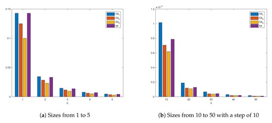
Figure 1. ${log}_4\left(CE\right)$ from Table 1 for methods $G{4}_1$, $G{4}_2$, $G{4}_3$, and $S4$ and different sizes of the system.

We have solved system (20) using methods $S4$ and $G{4}_1$ for $nx=20$. For the numerical performance, we use software Matlab R2017b with variable precision arithmetics of 1000 digits of mantissa.The results of the application of the methods for solving the nonlinear system are collected in Table 2 varying the value of $nt$ and $T_{max}$. For every performance, the iteration procedure stops when $\parallel F\left(x^{(k+1)}\right)\parallel <{10}^{-6}$ or the number of iterations reaches the number 50. The value of iter represents the mean number of iterations needed when all the columns have been calculated and the terms $a\left(b\right)$ represent the value $a·{10}^b$. Moreover, the elapsed time in seconds to obtain the solution for the problem after 10 (consecutive) executions is shown.

Table 2. Numerical results for $nx=20$ and different values of $T_{max}$ and $nt$.

${\mathit{T}}_{\mathit{m}\mathit{a}\mathit{x}}=0.5$	Method	nt	iter	$\parallel \mathit{F}\left({\mathit{x}}^{(\mathit{k}+1)}\right)\parallel$	e-time
	$S4$	100	16.0	9.6054 (−7)	397.1095
	$G{4}_1$		2.0	9.233 (−19)	93.5890
	$S4$	200	15.0	7.8637 (−7)	781.0227
	$G{4}_1$		2.0	7.2024 (−21)	152.5548
	$S4$	500	13.0	8.4237 (−7)	1.6520(03)
	$G{4}_1$		2.0	1.179 (−23)	515.5332
${\mathit{T}}_{\mathit{m}\mathit{a}\mathit{x}}=\mathbf{1}$	Method	nt	iter	$\parallel \mathit{F}\left({\mathit{x}}^{(\mathit{k}+1)}\right)\parallel$	e-time
	$S4$	100	17.96	8.1801 (−7)	838.7530
	$G{4}_1$		2.0	1.6217 (−16)	205.8390
	$S4$	200	16.37	6.6969 (−7)	880.8873
	$G{4}_1$		2.0	1.2656 (−18)	211.5296
	$S4$	500	14.592	7.1745 (−7)	1.9021(03)
	$G{4}_1$		2.0	2.0725 (−21)	518.8443
${\mathit{T}}_{\mathit{m}\mathit{a}\mathit{x}}=\mathbf{2}$	Method	nt	iter	$\parallel \mathit{F}\left({\mathit{x}}^{(\mathit{k}+1)}\right)\parallel$	e-time
	$S4$	100	19.5	7.2062 (−7)	529.8552
	$G{4}_1$		2.0	2.4203 (−14)	106.0159
	$S4$	200	17.98	9.6415 (−7)	965.8759
	$G{4}_1$		2.0	1.8728 (−16)	209.1218
	$S4$	500	16.11	6.3074 (−7)	2.0914(03)
	$G{4}_1$		2.0	3.0515 (−19)	513.5127

The results in Table 2 show the good performance of method $G{4}_1$ for solving the Fisher’s problem. Method $G{4}_1$ only needs two iterations to calculate a solution for the system, the mean number of iterations always being lower than that of method $S4$. For a fixed value of $T_{max}$, when $nt$ increases, so does the elapsed time, but the approximation to the solution is better since $\left|\right|F\left(x^{k+1}\right)\left|\right|$ is smaller. In addition, the e-time is lower for method $G{4}_1$, so it reaches the solution with more computational efficiency and arithmetical precision than the other scheme.

3.2. Application of Family GH to Nonlinear Test Systems

According to the results obtained in Table 1 for methods $G{4}_{1,2,3}$, the numerical experiments for family (13) are developed by using the following weight functions:

$$\begin{array}{ccc}\hfill G\left({\eta }_k\right)& =& I+{\eta }_k+2{\eta }_k^2+5{\eta }_k^3,\hfill \\ \hfill H\left({\tau }_k\right)& =& I+{\tau }_k+{\tau }_k^2+{\tau }_k^3,\hfill \end{array}$$

(23)

which satisfy conditions of Theorem 3.

To compare the features of our method with other schemes of the literature, the numerical tests are also performed on two iterative schemes of order 8 that can be found in [5,14]. The method is named $GH9$, for our iterative family using functions (23), $NLM8$ for [5], and $SLB8$, for [14]. The computational efficiency index and the number of functional evaluations of these methods are collected in Table 3.

Table 3. Funtional evaluations and computational efficiency index of methods $NLM8$, $SLB8$ and $GH9$.

Method	F	${\mathit{F}}^{\prime }$	nDD	d	s1	s2	Mv	op	Order	CE
$NLM8$	3	2	0	$2n^2+3n$	7	0	2	$\frac{1}{3}{n}^3+11n^2-\frac{2}{3}n$	8	$8^{1/(\frac{1}{3}{n}^3+13n^2+\frac{7}{3}n)}$
$SLB8$	3	2	0	$2n^2+3n$	2	9	6	$\frac{2}{3}{n}^3+17n^2-\frac{2}{3}n$	8	$8^{1/(\frac{2}{3}{n}^3+19n^2+\frac{7}{3}n)}$
$GH9$	2	1	2	$2n^2+n$	8	0	6	$\frac{1}{3}{n}^3+14n^2-\frac{1}{3}n$	9	$9^{1/(\frac{1}{3}{n}^3+16n^2+\frac{2}{3}n)}$

Method $GH9$ requires few functional evaluations, as low operational cost and has a competitive computational efficiency index (see Figure 2). We will see now that the numerical experiments confirm these results. For this purpose, methods $NLM8$, $SLB8$, and $GH9$ are applied to solve the following nonlinear systems:

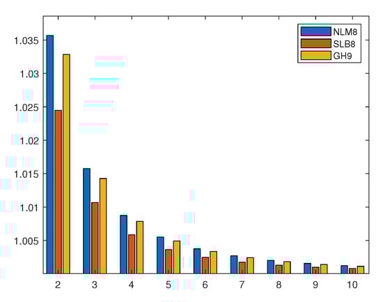
Figure 2. $CE$ from Table 3 for methods $NLM8$, $SLB8$, and $GH9$ for different sizes of the system.

(a)

$F_1(x,y)={\left(f_{11}(x,y),f_{12}(x,y)\right)}^T=0$, where

$$\left\{\begin{array}{c}{f}_{11}(x,y)=x^2-y-19,\hfill \\ f_{12}(x,y)=\frac{1}{6}{y}^3-x^2+y-17,\hfill \end{array}\right.$$

(b)

$F_2(x,y,z)={\left(f_{21}(x,y,z),f_{22}(x,y,z),f_{23}(x,y,z)\right)}^T=0$, such that

$$\left\{\begin{array}{c}{f}_{21}(x,y,z)=sin\left(x\right)+y^2+log\left(z\right)-7,\hfill \\ f_{22}(x,y,z)=3x+2^y-\frac{1}{z^3}+1,\hfill \\ f_{23}(x,y,z)=x+y-z-5,\hfill \end{array}\right.$$

(c)

$F_3(x,y,z)={\left(f_{31}(x,y,z),f_{32}(x,y,z),f_{33}(x,y,z)\right)}^T=0$, where

$$\left\{\begin{array}{c}{f}_{31}(x,y,z)=2x+y-z-4,\hfill \\ f_{32}(x,y,z)=2y+z+x-4,\hfill \\ f_{33}(x,y,z)=xyz-1.\hfill \end{array}\right.$$

The results obtained from applying the methods for solving the nonlinear systems are collected in Table 4, Table 5 and Table 6. The stopping criteria now is a difference between two consecutive iterates lower than ${10}^{-200}$ or the condition $\parallel F\left(x^{(k+1)}\right)\parallel <{10}^{-200}$ with a maximum number of iterations of 50. The results have been calculated using Matlab R2017b with variable precision arithmetics of 2000 digits of mantissa. In this way, the numerical noise is far enough to not affect the final result. The approximated computational order of convergence [15] represents an approximation of the order of convergence of each method.

Table 4. Numerical results for $F_1(x,y)$.

Method	${\mathit{x}}^{\left(0\right)}$	Iter	$\parallel \mathit{F}\left({\mathit{x}}^{(\mathit{k}+1)}\right)\parallel$	ACOC
$NLM8$	[7 7]	3	1.929 (−201)	6.9500
$SLB8$		3	1.433 (−378)	7.8627
$GH9$		3	4.151 (−343)	8.2992
$NLM8$	[4 −4.5]	47	1.255 (−865)	6.0711
$SLB8$		36	3.522 (−203)	7.7505
$GH9$		20	1.164 (−1218)	7.9956
$NLM8$	[−10 −7.5]	20	3.371 (−501)	6.4336
$SLB8$		5	6.248 (−1248)	8.0000
$GH9$		4	1.722 (−416)	8.1830

Table 5. Numerical results for $F_2(x,y,z)$.

Method	${\mathit{x}}^{\left(0\right)}$	Iter	$\parallel \mathit{F}\left({\mathit{x}}^{(\mathit{k}+1)}\right)\parallel$	ACOC
$NLM8$	[−1.5 −1.5 −1.5]	4	7.484 (−633)	6.3006
$SLB8$		4	3.902 (−1402)	7.9274
$GH9$		4	7.286 (−1127)	8.0749
$NLM8$	[0 −1 −1.5]	5	9.291 (−1174)	5.892
$SLB8$		4	2.557 (−1318)	7.9291
$GH9$		4	1.064 (−425)	8.5315
$NLM8$	[3 4 5]	5	1.200 (−958)	5.9817
$SLB8$		5	1.306 (−839)	8.0606
$GH9$		4	3.982 (−350)	8.3187

Table 6. Numerical results for $F_3(x,y,z)$.

Method	${\mathit{x}}^{\left(0\right)}$	Iter	$\parallel \mathit{F}\left({\mathit{x}}^{(\mathit{k}+1)}\right)\parallel$	ACOC
$NLM8$	[−1 1 2]	4	2.587 (−412)	7.8793
$SLB8$		13	2.419 (−854)	7.9973
$GH9$		4	6.575 (−616)	8.0173
$NLM8$	[−0.6 0.8 2.7]	34	1.393 (−290)	7.7554
$SLB8$		14	7.066 (−785)	7.9959
$GH9$		4	2.445 (−511)	8.0092
$NLM8$	[−2.5 −1 1]	15	1.667 (−420)	7.9179
$SLB8$		5	7.361 (−1165)	7.9992
$GH9$		4	2.522 (−325)	8.3981

The ACOC [15] is the approximated computational order of convergence defined as

$$p\approx ACOC=\frac{ln\left(\left|\right|x^{(k+1)}-x^{\left(k\right)}\left|\right|/\left|\right|x^{\left(k\right)}-x^{(k-1)}\left|\right|\right)}{ln\left(\left|\right|x^{\left(k\right)}-x^{(k-1)}\left|\right|/\left|\right|x^{(k-1)}-x^{(k-2)}\left|\right|\right)}.$$

It is a computational approximation of the theoretical order.

For every nonlinear system, the higher value of the ACOC is for the GH family, as expected. In general, our proposed scheme converges in less iterations than the other tested methods with very competitive error estimates.

4. Conclusions

Two families of iterative methods for solving nonlinear systems of equations have been introduced, the first one being a multidimensional extension of a previous scalar class of iterative methods. Both schemes are designed via the matrix weight functions procedure with only one evaluation of the Jacobian and its estimation using divided differences for systems. Two more steps are added to the fourth-order class, holding the Jacobian matrix evaluated in the same step, allowing us to reach order of convergence 9 for the GH family. The numerical tests confirm the quality of the iterative schemes for solving systems of equations of non-small size, improving the results of several methods in the literature.

References

- Petković, M.S.; Neta, B.; Petković, L.D.; Džunić, J. Multipoint Methods for Solving Nonlinear Equations: A survey. App. Math. Comput. 2014, 226, 635–660. [Google Scholar]
- Cordero, A.; Torregrosa, J.R. On the Design of Optimal Iterative Methods for Solving Nonlinear Equations. In Advances in Iterative Methods for Nonlinear Equations; Amat, S., Busquier, S., Eds.; Springer: Cham, Switzerland, 2016; pp. 79–111. [Google Scholar]
- Kung, H.T.; Traub, J.F. Optimal order of one-point and multipoint iteration. J. Assoc. Comput. Math. 1974, 21, 643–651. [Google Scholar] [CrossRef]
- Cordero, A.; Gómez, E.; Torregrosa, J.R. Efficient high-order iterative methods for solving nonlinear systems and their application on heat conduction problems. Complexity 2017, 2017, 6457532. [Google Scholar] [CrossRef]
- Sharma, J.; Arora, H. Improved Newton-like methods for solving systems of nonlinear equations. SeMA J. 2017, 74, 147–163. [Google Scholar] [CrossRef]
- Amiri, A.; Cordero, A.; Darvishi, M.; Torregrosa, J. Stability analysis of a parametric family of seventh-order iterative methods for solving nonlinear systems. App. Math. Comput. 2018, 323, 43–57. [Google Scholar] [CrossRef]
- Cordero, A.; Hueso, J.L.; Martínez, E.; Torregrosa, J.R. A modified Newton-Jarratt’s composition. Numer. Algor. 2010, 55, 87–99. [Google Scholar] [CrossRef]
- Chicharro, F.I.; Cordero, A.; Garrido, N.; Torregrosa, J.R. Wide stability in a new family of optimal fourth-order iterative methods. Comput. Math. Methods 2019, 1, e1023. [Google Scholar] [CrossRef]
- Artidiello, S. Diseño, Implementación y Convergencia de Métodos Iterativos Para Resolver Ecuaciones y Sistemas No Lineales Utilizando Funciones Peso. Ph.D. Thesis, Servicio de publicaciones Universidad Politécnica de Valencia, Valencia, Spain, 2014. [Google Scholar]
- Ortega, J.M.; Reinhboldt, W.C. Iterative Solution of Nonlinear Equations in Several Variables; Academic Press: Cambridge, MA, USA, 1970. [Google Scholar]
- Fisher, R.A. The wave of advance of advantageous genes. Ann. Eugen. 1933, 7, 353–369. [Google Scholar] [CrossRef]
- Sharma, J.; Guha, R.; Sharma, R. An efficient fourth order weighted-Newton method for systems of nonlinear equations. Numer. Algor. 2013, 62, 307–323. [Google Scholar] [CrossRef]
- Ostrowski, A. Solution of Equations and Systems of Equations; Prentice-Hall: Upper Saddle River, NJ, USA, 1964. [Google Scholar]
- Soleymani, F.; Lotfi, T.; Bakhtiari, P. A multi-step class of iterative methods for nonlinear systems. Optim. Lett. 2014, 8, 1001–1015. [Google Scholar] [CrossRef]
- Cordero, A.; Torregrosa, J.R. Variants of Newton’s method using fifth order quadrature formulas. Appl. Math. Comput. 2007, 190, 686–698. [Google Scholar] [CrossRef]
© 2019 by the authors. Licensee MDPI, Basel, Switzerland. This article is an open access article distributed under the terms and conditions of the Creative Commons Attribution (CC BY) license (http://creativecommons.org/licenses/by/4.0/).