Analysis of Structure-Preserving Discrete Models for Predator-Prey Systems with Anomalous Diffusion

Abstract

In this work, we investigate numerically a system of partial differential equations that describes the interactions between populations of predators and preys. The system considers the effects of anomalous diffusion and generalized Michaelis–Menten-type reactions. For the sake of generality, we consider an extended form of that system in various spatial dimensions and propose two finite-difference methods to approximate its solutions. Both methodologies are presented in alternative forms to facilitate their analyses and computer implementations. We show that both schemes are structure-preserving techniques, in the sense that they can keep the positive and bounded character of the computational approximations. This is in agreement with the relevant solutions of the original population model. Moreover, we prove rigorously that the schemes are consistent discretizations of the generalized continuous model and that they are stable and convergent. The methodologies were implemented efficiently using MATLAB. Some computer simulations are provided for illustration purposes. In particular, we use our schemes in the investigation of complex patterns in some two- and three-dimensional predator–prey systems with anomalous diffusion.

1. Introduction

The investigation of the interactions between populations of predators and preys in nature is a highly transited topic of research in applied mathematics currently. Indeed, this area of research has proven to be extremely fruitful in view of the wide range of possible scenarios that merit investigation. As examples, we can mention studies that report on the modeling and analysis of predator–prey models with disease in the prey [1], the analysis of stochastic systems with modified Leslie–Gower and Holling-type schemes [2], the dynamic behaviors of Lotka–Volterra predator–prey models that incorporate predator cannibalism [3], the analysis of diffusive predator–prey systems with Michaelis–Menten-type predator harvesting [4], synthetic Escherichia coli predator–prey ecosystems [5], the analytical investigation of stage-structured predator–prey models depending on maturation delay and death rate [6], and non-autonomous ratio dependent models with Holling-type functional response with temporal delay [7], among other interesting topics [8].

It is worth pointing out that the investigation has focused mainly on the analytical aspects of the problem [9]. However, the literature reports on various numerical methods that have been designed explicitly to solve efficiently various predator–prey systems. For instance, there are studies on dynamically consistent nonstandard finite-difference schemes to solve predator–prey models [10], while some of those methods have been implemented in MATLAB with the aim of being available to the scientific community [11]. There are also some positive and elementary stable nonstandard schemes that have been applied to solve predator–prey systems [12], modified Leslie–Gower and Holling-type II schemes with temporal delay [13], nonstandard numerical schemes for predator–prey models having a generalized functional response [14], as well as positivity and boundedness-preserving methods for some space-time fractional predator–prey models [15]. Of course, the investigation in this area is still an important topic of research.

To date, fractional differential equations have been used in mathematical systems to produce more accurate models for physical problems [16]. Various applications have been proposed in a number of areas [17,18], including various problems in viscoelasticity [19], some phenomena related to thermoelasticity [20], in continuous-time financing problems [21], in the dynamics of self-similar proteins [22], relativistic quantum mechanics [23], the control of diabetes [24], the theory of solitons [25], and plasma physics [26]. Moreover, the research on predator–prey systems has also benefited from the recent progresses in fractional calculus. Recent reports have studied fractional models of predators and preys that incorporate feedback control and a constant prey refuge [27], bifurcations of delayed fractional systems with incommensurate orders [28], periodic solutions and control optimization of models with two types of harvesting [29], and fractional predator–prey systems with delay and Holling type-II functional response [30], among other recent works available in the literature.

It is well known that the complexity of fractional systems is much higher than the complexity of integer-order systems. From that point of view, it is necessary to propose efficient numerical methods to solve meaningful fractional-order systems [31]. In that sense, the literature provides some reports to calculate the solutions of fractional models. For instance, there are some computational schemes to approximate the solutions of fractional differential equations using fractional centered differences [32], the diffusion equation with fractional derivatives in time [33], the multidimensional fractional Schrödinger equation [34], the nonlinear Korteweg–de Vries–Burgers equation with fractional derivatives [35], and the two-dimensional fractional FitzHugh–Nagumo monodomain model [36], among others [37]. However, the search for better algorithms to simulate fractional systems (which provide fast results with minimal computer resources) is still an open problem of research.

Motivated by this background, we will consider a predator–prey system with fractional diffusion that considers reaction functionals. The reaction terms will follow Michaelis–Menten laws [38], while the diffusion considered in this work will be of the Riesz type [39]. It is worth pointing out here that the choice of the fractional derivative type obeys various mathematical and physical reasons. Most importantly, it has been recently found that Riesz fractional derivatives can be obtained from systems with long range interactions in some continuous-limit approximations [40]. In order to reach some level of generality, we will consider an extended form of the predator–prey system under investigation, considering sufficiently general reaction functions and various spatial dimensions. In light of the complexity to solve exactly such a model, we will propose some finite-difference methods based on the concept of fractional centered differences [41]. Motivated then by the fact that the relevant solutions of the system are positive and bounded functions, we will prove that our discretizations are capable of preserving these features of the numerical solutions. Moreover, we will prove rigorously the consistency, the stability, and the convergence of the methodologies. Some applications will be provided to illustrate the usefulness of our models and our implementations.

This manuscript is sectioned as follows. In Section 2, we provide the mathematical system under study. The system consists of two partial differential equations with coupled reaction terms and Riesz fractional diffusion. We introduce therein the definition of fractional centered differences, which is the cornerstone to provide a discretization of our model. In turn, Section 3 presents the discrete notation along with two finite-difference schemes to estimate the solutions of the continuous system. It is worth noting that one of the models will be an implicit scheme, while the other is explicit. These numerical methods will be analyzed structurally in Section 4. As the most important results from that section, we establish the existence, uniqueness, positivity, and boundedness of the solutions for both methods. Section 5 is devoted to establishing the numerical properties of the schemes, including the consistency, stability, and convergence. Some numerical applications are provided in Section 6, and we close this manuscript with some concluding observations.

2. Preliminaries

Throughout, assume that $a_i$ and $b_i$ are real numbers such that $a_i<b_i$, for each $i=1,2,3$. Let $T>0$ represent a fixed time. We define $\Omega =(a_1,b_1)\times (a_2,b_2)\times (a_3,b_3)$ and ${\Omega }_T=\Omega \times (0,T)$ and use $\overline{\Omega }$ and ${\overline{\Omega }}_T$ to represent the closures of $\Omega$ and ${\Omega }_T$, respectively. In this manuscript, $u:{\overline{\Omega }}_T\to \mathbb{R}$ and $v:{\overline{\Omega }}_T\to \mathbb{R}$ represent sufficiently smooth functions, and define $x=(x_1,x_2,x_3)\in \Omega$.

Definition 1

(Podlubny [42]). Assume that $f:\mathbb{R}\to \mathbb{R}$, and suppose that $n\in \mathbb{N}\cup \left\{0\right\}$ and $\alpha \in \mathbb{R}$ are such that $n-1<\alpha <n$. If it exists, we introduce the fractional derivative in the sense of Riesz of the function f of order α at the point $x\in \mathbb{R}$ as:

$$\frac{d^{\alpha }f(x)}{{d|x|}^{\alpha }}=\frac{-1}{2cos(\frac{\pi \alpha }{2})\Gamma (n-\alpha )}\frac{d^n}{d{x}^n}{\int }_{-\infty }^{\infty }\frac{f(\xi )d\xi }{{|x-\xi |}^{\alpha +1-n}}.$$

(1)

Here, the Gamma function is given by:

$$\Gamma \left(z\right)={\int }_0^{\infty }{s}^{z-1}{e}^{-s}ds,\forall z>0.$$

(2)

Definition 2.

Suppose that$u:{\overline{\Omega }}_T\to \mathbb{R}$; assume that$\alpha >-1$; and let$n\in \mathbb{Z}$satisfy$n-1<\alpha \le n$. If they exist, the Riesz space-fractional derivatives of the function u of order α with respect to$x_1$,$x_2$, and$x_3$at the point$\left(x,t\right)\in {\Omega }_T$are respectively defined by:

$$\begin{array}{cc}\hfill \frac{{\partial }^{\alpha }u}{\partial {|x_1|}^{\alpha }}(x,t)& =\frac{-1}{2cos\left(\frac{\pi \alpha }{2}\right)\Gamma \left(n-\alpha \right)}\frac{{\partial }^n}{\partial x_1^n}{\int }_{a_1}^{b_1}\frac{u\left(\xi ,x_2,x_3,t\right)d\xi }{{|x_1-\xi |}^{\alpha +1-n}},\hfill \end{array}$$

(3)

$$\begin{array}{cc}\hfill \frac{{\partial }^{\alpha }u}{\partial {|x_2|}^{\alpha }}(x,t)& =\frac{-1}{2cos\left(\frac{\pi \alpha }{2}\right)\Gamma \left(n-\alpha \right)}\frac{{\partial }^n}{\partial x_2^n}{\int }_{a_2}^{b_2}\frac{u\left(x_1,\xi ,x_3,t\right)d\xi }{{|x_2-\xi |}^{\alpha +1-n}},\hfill \end{array}$$

(4)

$$\begin{array}{cc}\hfill \frac{{\partial }^{\alpha }u}{\partial {|x_3|}^{\alpha }}(x,t)& =\frac{-1}{2cos\left(\frac{\pi \alpha }{2}\right)\Gamma \left(n-\alpha \right)}\frac{{\partial }^n}{\partial x_3^n}{\int }_{a_3}^{b_3}\frac{u\left(x_1,x_2,\xi ,t\right)d\xi }{{|x_3-\xi |}^{\alpha +1-n}}.\hfill \end{array}$$

(5)

For the remainder of this paper, we will let a, c, d, $D_1$, and $D_2$ be positive; suppose that $b\in \mathbb{R}$, and let $\alpha ,\beta \in \mathbb{R}$ be such that $1<\alpha \le 2$ and $1<\beta \le 2$. Let ${\varphi }_u:\overline{\Omega }\to \mathbb{R}$ and ${\varphi }_v:\overline{\Omega }\to \mathbb{R}$ be two functions that physically describe the initial conditions for populations of prey and predator, respectively. Under these conventions, the problem under investigation is the predator–prey model with Allee effects and diffusion of fractional order, which is described by:

$$\begin{array}{c}{\displaystyle \frac{\partial u(x,t)}{\partial t}=au\left(u-b\right)\left(1-u\right)-\frac{uv}{u+v}+D_1\sum _{i=1}^3\frac{{\partial }^{\alpha }u(x,t)}{\partial |x_i{|}^{\alpha }},\forall (x,t)\in {\Omega }_T,}\hfill \\ {\displaystyle \frac{\partial v(x,t)}{\partial t}=\frac{cuv}{u+v}-dv+D_2\sum _{i=1}^3\frac{{\partial }^{\beta }u(x,t)}{\partial |x_i{|}^{\beta }},\forall (x,t)\in {\Omega }_T,}\hfill \\ \mathrm{such} \mathrm{that}\left\{\begin{array}{cc}u(x,0)={\varphi }_u(x),\hfill & \forall x\in \Omega ,\hfill \\ v(x,0)={\varphi }_v(x),\hfill & \forall x\in \Omega .\hfill \end{array}\right.\hfill \end{array}$$

(6)

Convey that $u=u(x,t)$ and $v=v(x,t)$ for simplicity. The model (6) is a Michaelis–Menten-type reaction-diffusion predator–prey system where the diffusion is anomalous. Here, $u(x,t)$ and $v(x,t)$ represent the normalized densities of the prey and the predator, respectively, at the point $x\in \Omega$ and time $t\ge 0$. The relative constant a is the intrinsic rate of growth of the prey; $b\in (-1,1)$ is the Allee effect; $c\in (0,1]$ denotes the rate of the energy rate from the prey to the predator; and d is the relative rate of death of the predator population. Meanwhile, $D_1$ and $D_2$ are non-negative constants that represent the speed of individual movements of u and v, respectively [43].

Notice that we can rewrite the system (6) in generalized form as:

$$\begin{array}{c}{\displaystyle \frac{\partial u(x,t)}{\partial t}=auF(u)-u{G}^u(u,v)+D_1\sum _{i=1}^3\frac{{\partial }^{\alpha }u(x,t)}{\partial |x_i{|}^{\alpha }},\forall (x,t)\in {\Omega }_T,}\hfill \\ {\displaystyle \frac{\partial v(x,t)}{\partial t}=cv{G}^v(u,v)-dv+D_2\sum _{i=1}^3\frac{{\partial }^{\beta }v(x,t)}{\partial |x_i{|}^{\beta }},\forall (x,t)\in {\Omega }_T,}\hfill \\ \mathrm{such} \mathrm{that}\left\{\begin{array}{cc}u(x,0)={\varphi }_u(x),\hfill & \forall x\in \Omega ,\hfill \\ v(x,0)={\varphi }_v(x),\hfill & \forall x\in \Omega .\hfill \end{array}\right.\hfill \end{array}$$

(7)

where the function F depends on u, while $G^u$ and $G^v$ depend on both u and v. It is easy to see that the system (7) reduces to the population model (6) when F, $G^u$, and $G^v$ have the following expressions with $u,v\in {\mathbb{R}}^{+}\cup \left\{0\right\}$:

$$\begin{array}{c}\hfill F(u)=(u-b)(1-u),G^u(u,v)=\frac{v}{u+v},G^v(u,v)=\frac{u}{u+v}.\end{array}$$

(8)

Moreover, if $\alpha =\beta =2$, $D_1=D_2=0$, $F(u,v)=1$, $G^u=v$, and $G^v=u$, then (7) reduces to the well-known Lotka–Volterra system.

We recall the following definition from the literature. It will be an essential tool to provide consistent discretizations of the general fractional problem (7).

Definition 3

(Ortigueira [41]). Let $f:\mathbb{R}\to \mathbb{R}$, and assume that $h>0$ and $\alpha >-1$. The centered difference of fractional order α of the function f at x is given (when it exists) as:

$${\Delta }_h^{(\alpha )}f(x)=\sum _{k=-\infty }^{\infty }{g}_k^{(\alpha )}f(x-kh),\forall x\in \mathbb{R},$$

(9)

where:

$$g_k^{(\alpha )}=\frac{{(-1)}^k\Gamma (\alpha +1)}{\Gamma (\frac{\alpha }{2}-k+1)\Gamma (\frac{\alpha }{2}+k+1)},\forall k\in \mathbb{Z}.$$

(10)

Lemma 1

(Wang et al. [44]). Let $0<\alpha \le 2$ and $\alpha \ne 1$.

(a)

The following iterative formulas hold:

$$\begin{array}{cc}\hfill g_0^{(\alpha )}& {\displaystyle =\frac{\Gamma (\alpha +1)}{{[\Gamma (\frac{\alpha }{2}+1)]}^2},}\hfill \end{array}$$

(11)

$$\begin{array}{cc}\hfill g_{k+1}^{(\alpha )}& {\displaystyle =\left(1-\frac{\alpha +1}{\alpha /2+k+1}\right)g_k,\forall k\in \mathbb{N}\cup \left\{0\right\}.}\hfill \end{array}$$

(12)

(b)

$g_0^{(\alpha )}>0$.

(c)

$g_k^{(\alpha )}=g_{-k}^{(\alpha )}<0$for all$k\ne 0$.

(d)

${\displaystyle \sum _{k=-\infty }^{\infty }{g}_k^{(\alpha )}=0}$.

Lemma 2

(Wang et al. [44]). Let $0<\alpha \le 2$ and $\alpha \ne 1$, and suppose that $f\in {\mathcal{C}}^5(\mathbb{R})$ is a function whose derivatives up to order five are all integrable. For almost all $x\in \mathbb{R}$,

$$-\frac{{\Delta }_h^{\alpha }f(x)}{h^{\alpha }}=\frac{{\partial }^{\alpha }f(x)}{{\partial |x|}^{\alpha }}+\mathcal{O}(h^2).$$

(13)

3. Numerical Models

The purpose of this section is to propose two different methods based on finite-differences to approximate the solutions of (7). For the sake of convenience, we consider only the two-dimensional form of (7), which reads as follows:

$$\begin{array}{c}{\displaystyle \frac{\partial u(x,t)}{\partial t}=auF(u)-u{G}^u(u,v)+D_1\sum _{i=1}^2\frac{{\partial }^{\alpha }u(x,t)}{\partial |x_i{|}^{\alpha }},\forall (x,t)\in {\Omega }_T,}\hfill \\ {\displaystyle \frac{\partial v(x,t)}{\partial t}=cv{G}^v(u,v)-dv+D_2\sum _{i=1}^2\frac{{\partial }^{\beta }v(x,t)}{\partial |x_i{|}^{\beta }},\forall (x,t)\in {\Omega }_T,}\hfill \\ \mathrm{such} \mathrm{that}\left\{\begin{array}{cc}u(x,0)={\varphi }_u(x),\hfill & \forall x\in \Omega ,\hfill \\ v(x,0)={\varphi }_v(x),\hfill & \forall x\in \Omega .\hfill \end{array}\right.\hfill \end{array}$$

(14)

It is worth pointing out that an analysis of the three-dimensional model is also feasible, though it would require additional nomenclature. We preferred to carry out the full description and analysis in the two-dimensional case for the sake of a better explanation.

Agree that $I_p=\{1,2,\cdots ,p\}$ and ${\overline{I}}_p=I_p\cup \left\{0\right\}$, for all $p\in \mathbb{N}$. Let $M,N,K\in \mathbb{N}$, and introduce uniform partitions of $[a_1,b_1]$ and $[a_2,b_2]$, respectively, denoted by:

$$\begin{array}{c}\hfill \begin{array}{c}{a}_1=x_{1,0}<x_{1,1}<\dots <x_{1,m}<\dots <x_{1,M}=b_1,\forall m\in {\overline{I}}_M,\\ a_2=x_{2,0}<x_{2,1}<\dots <x_{2,n}<\dots <x_{2,N}=b_2,\forall n\in {\overline{I}}_N.\end{array}\end{array}$$

(15)

Obviously, $x_{1,m}=a_1+h_{x_1}m$ and $x_{2,n}=a_2+h_{x_2}n$ for each $m\in {\overline{I}}_M$ and $n\in {\overline{I}}_N$. In this case, the partition norms in the $x_1$ and $x_2$ directions are $h_{x_1}=(b_1-a_1)/M$ and $h_{x_2}=(b_2-a_2)/N$, respectively.

In a similar fashion, we fix a (not necessarily uniform) partition for the interval $[0,T]$, which will be represented by:

$$\begin{array}{c}\hfill \begin{array}{c}0=t_0<t_1<\dots <t_k<\dots <t_K=T,\forall k\in {\overline{I}}_K.\hfill \end{array}\end{array}$$

(16)

For each $k\in {\overline{I}}_{K-1}$, we let ${\tau }_k=t_{k+1}-t_k$. Numerically, we define $u_{m,n}^k$ and $v_{m,n}^k$, respectively, as the approximations to the analytical solutions u and v of (14) at the point $(x_{1,m},x_{2,n},t_k)$ for each $m\in {\overline{I}}_M$, $n\in {\overline{I}}_N$, and $k\in {\overline{I}}_K$.

Definition 4.

Let$\alpha \in (0,1)\cup (1,2]$. Define the discrete linear operators:

$$\begin{array}{ccc}\hfill {\displaystyle {\delta }_{x_1}^{(\alpha )}{u}_{m,n}^k=-\frac{1}{h_{x_1}^{\alpha }}\sum _{i=0}^M{g}_{m-i}^{(\alpha )}{u}_{i,n}^k,}& \hfill & \hfill {\delta }_{x_2}^{(\alpha )}{u}_{m,n}^k=-\frac{1}{h_{x_2}^{\alpha }}\sum _{i=0}^N{g}_{n-i}^{(\alpha )}{u}_{m,i}^k,\end{array}$$

(17)

$$\begin{array}{ccc}\hfill {\displaystyle {\delta }_{x_1}^{(\alpha )}{v}_{m,n}^k=-\frac{1}{h_{x_1}^{\alpha }}\sum _{i=0}^M{g}_{m-i}^{(\alpha )}{v}_{i,n}^k,}& \hfill & \hfill {\delta }_{x_2}^{(\alpha )}{v}_{m,n}^k=-\frac{1}{h_{x_2}^{\alpha }}\sum _{i=0}^N{g}_{n-i}^{(\alpha )}{v}_{m,i}^k.\end{array}$$

(18)

By Lemma 2, the discrete operators introduced above provide approximations of second order to the Riesz spatial derivatives of the functions u and v, with respect to $x_1$ and $x_2$ at the point $(x_{1,m},x_{2,n},t_k)$. For the remainder of this work and without loss of generality, we assume that the partition of the interval $[0,T]$ is uniform, in which case ${\tau }_k=\tau \in {\mathbb{R}}^{+}$, for each $k\in {\overline{I}}_{K-1}$. This assumption will be imposed only for the sake of convenience in the use of our notation.

3.1. Explicit Method

We present here an explicit scheme to approximate the solutions of (14). In the first stage, we introduce additional discrete operators to describe the scheme. The nomenclature presented in Section 2 will be observed throughout this section.

Definition 5.

Let w be any of u or v. For each$m\in {\overline{I}}_M$,$n\in {\overline{I}}_N$, and$k\in I_{K-1}$, we introduce the standard linear operators:

$${\delta }_t{w}_{m,n}^k=\frac{w_{m,n}^{k+1}-w_{m,n}^k}{\tau },$$

(19)

Recall now that the operator (19) yields a first-order estimate of the partial derivative of w with respect to time at $(x_{1,m},x_{2,n},t)$, for each $m\in {\overline{I}}_M$, $n\in {\overline{I}}_N$, and $k\in I_{K-1}$. Substituting the differential operators of (7) for their finite-difference approximations, we obtain the following discrete model to approximate the solutions of (14):

$$\begin{array}{c}{\displaystyle {\delta }_t{u}_{m,n}^k=aF(u_{m,n}^k)u_{m,n}^k-G^u(u_{m,n}^k,v_{m,n}^k)u_{m,n}^k+D_1\sum _{i=1}^2{\delta }_{x_i}^{(\alpha )}{u}_{m,n}^k,}\hfill \\ {\displaystyle {\delta }_t{v}_{m,n}^k=c{G}^v(u_{m,n}^k,v_{m,n}^k)v_{m,n}^k-d{v}_{m,n}^k+D_2\sum _{i=1}^2{\delta }_{x_i}^{(\beta )}{v}_{m,n}^k,}\hfill \\ \mathrm{such} \mathrm{that}\left\{\begin{array}{cc}{u}_{m,n}^0={\varphi }_{u,m,n}^0,\hfill & \forall (m,n)\in {\overline{I}}_M\times {\overline{I}}_N,\hfill \\ v_{m,n}^0={\varphi }_{v,m,n}^0,\hfill & \forall (m,n)\in {\overline{I}}_M\times {\overline{I}}_N.\hfill \end{array}\right.\hfill \end{array}$$

(20)

Here, the difference equations are valid for each $m\in {\overline{I}}_M$, $n\in {\overline{I}}_N$, and $k\in {\overline{I}}_{K-1}$.

Substituting then the expressions of the discrete operators into (20), we obtain an alternative representation of our finite-difference scheme. More precisely, let:

$$R_i^u=\frac{\tau D_1}{h_{x_i}^{\alpha }}\mathrm{and}{R}_i^v=\frac{\tau D_2}{h_{x_i}^{\beta }},$$

(21)

for each $i=1,2$ and $\alpha ,\beta \in (1,2]$. After some algebraic operations, it is easy to check that the recursive equations of (20) can be rewritten equivalently as:

$$\begin{array}{c}{\displaystyle u_{m,n}^{k+1}={\mathfrak{a}}_{m,n}^k{u}_{m,n}^k+\sum _{\begin{array}{c}i=0\\ i\ne m\end{array}}^M{\mathfrak{b}}_{m,i}{u}_{i,n}^k+\sum _{\begin{array}{c}i=0\\ i\ne n\end{array}}^N{\mathfrak{c}}_{n,i}{u}_{m,i}^k,}\hfill \\ {\displaystyle v_{m,n}^{k+1}={\mathfrak{e}}_{m,n}^k{v}_{m,n}^k+\sum _{\begin{array}{c}i=0\\ i\ne m\end{array}}^M{\mathfrak{f}}_{m,i}{v}_{i,n}^k+\sum _{\begin{array}{c}i=0\\ i\ne n\end{array}}^N{\mathfrak{g}}_{n,i}{v}_{m,i}^k,}\hfill \end{array}$$

(22)

where:

$$\begin{array}{cc}\hfill {\mathfrak{a}}_{m,n}^k& =1+a\tau F(u_{m,n}^k)-\tau G^u(u_{m,n}^k,v_{m,n}^k)-R_1^u{g}_0^{(\alpha )}-R_2^u{g}_0^{(\alpha )},\hfill \end{array}$$

(23)

$$\begin{array}{cc}\hfill {\mathfrak{b}}_{m,i}& =-R_1^u{g}_{m-i}^{(\alpha )},\hfill \end{array}$$

(24)

$$\begin{array}{cc}\hfill {\mathfrak{c}}_{n,i}& =-R_2^u{g}_{n-i}^{(\alpha )},\hfill \end{array}$$

(25)

$$\begin{array}{cc}\hfill {\mathfrak{e}}_{m,n}^k& =1+\tau c{G}^v(u_{m,n}^k,v_{m,n}^k)-d\tau -R_1^v{g}_0^{(\beta )}-R_2^v{g}_0^{(\beta )},\hfill \end{array}$$

(26)

$$\begin{array}{cc}\hfill {\mathfrak{f}}_{m,i}& =-R_1^v{g}_{m-i}^{(\beta )},\hfill \end{array}$$

(27)

$$\begin{array}{cc}\hfill {\mathfrak{g}}_{n,i}& =-R_2^v{g}_{n-i}^{(\beta )}.\hfill \end{array}$$

(28)

Let ${}^{\top }$ represent matrix transposition. Observe then that (22) can be represented in an equivalent vector form. Indeed, let $k\in {\overline{I}}_K$ and $j\in {\overline{I}}_M$, and define the $(N+1)$-dimensional vectors:

$$\begin{array}{cc}\hfill u_j^k& ={(u_{j,0}^k,u_{j,1}^k,\cdots ,u_{j,N-1}^k,u_{j,N}^k)}^{\top },\hfill \end{array}$$

(29)

$$\begin{array}{cc}\hfill v_j^k& ={(v_{j,0}^k,v_{j,1}^k,\cdots ,v_{j,N-1}^k,v_{j,N}^k)}^{\top },\hfill \end{array}$$

(30)

$$\begin{array}{cc}\hfill {\varphi }_{u,j}^0& ={({\varphi }_{u,j,0}^0,{\varphi }_{u,j,1}^0,\cdots ,{\varphi }_{u,j,N-1}^0,{\varphi }_{u,j,N}^0)}^{\top },\hfill \end{array}$$

(31)

$$\begin{array}{cc}\hfill {\varphi }_{v,j}^0& ={({\varphi }_{v,j,0}^0,{\varphi }_{v,j,1}^0,\cdots ,{\varphi }_{v,j,N-1}^0,{\varphi }_{v,j,N}^0)}^{\top }.\hfill \end{array}$$

(32)

With these conventions, we introduce the $(M+1)\times (N+1)$-dimensional vectors:

$$\begin{array}{cc}\hfill u^k& =u_0^k\oplus u_1^k\oplus \cdots \oplus u_M^k,\hfill \end{array}$$

(33)

$$\begin{array}{cc}\hfill v^k& =v_0^k\oplus v_1^k\oplus \cdots \oplus v_M^k,\hfill \end{array}$$

(34)

$$\begin{array}{cc}\hfill {\varphi }_u^0& ={\varphi }_{u,0}^0\oplus {\varphi }_{u,1}^0\oplus \cdots \oplus {\varphi }_{u,M}^0,\hfill \end{array}$$

(35)

$$\begin{array}{cc}\hfill {\varphi }_v^0& ={\varphi }_{u,0}^1\oplus {\varphi }_{u,1}^1\oplus \cdots \oplus {\varphi }_{u,M}^1,\hfill \end{array}$$

(36)

where ⊕ represents the vector operation of juxtaposition.

The following are all matrices of dimension $(N+1)\times (N+1)$, for each $m\in {\overline{I}}_M$ and $k\in {\overline{I}}_{K-1}$:

$$\begin{array}{ccc}\hfill B_{m,i}& =\left(\begin{array}{ccccc}{\mathfrak{b}}_{m,i}& 0& 0& \cdots & 0\\ 0& {\mathfrak{b}}_{m,i}& 0& \cdots & 0\\ 0& 0& {\mathfrak{b}}_{m,i}& \cdots & 0\\ ⋮& ⋮& ⋮& \ddots & ⋮\\ 0& 0& 0& \cdots & {\mathfrak{b}}_{m,i}\end{array}\right),\hfill & \hfill C_m^k=\left(\begin{array}{ccccc}{\mathfrak{a}}_{m,0}^k& {\mathfrak{c}}_{0,1}& {\mathfrak{c}}_{0,2}& \cdots & {\mathfrak{c}}_{0,N}\\ {\mathfrak{c}}_{1,0}& {\mathfrak{a}}_{m,1}^k& {\mathfrak{c}}_{1,2}& \cdots & {\mathfrak{c}}_{1,N}\\ {\mathfrak{c}}_{2,0}& {\mathfrak{c}}_{2,1}& {\mathfrak{a}}_{m,2}^k& \cdots & {\mathfrak{c}}_{2,N}\\ ⋮& ⋮& ⋮& \ddots & ⋮\\ {\mathfrak{c}}_{N,0}& {\mathfrak{c}}_{N,1}& {\mathfrak{c}}_{N,2}& \cdots & {\mathfrak{a}}_{m,N}^k\end{array}\right),\end{array}$$

(37)

$$\begin{array}{ccc}\hfill F_{m,i}& =\left(\begin{array}{ccccc}{\mathfrak{f}}_{m,i}& 0& 0& \cdots & 0\\ 0& {\mathfrak{f}}_{m,i}& 0& \cdots & 0\\ 0& 0& {\mathfrak{f}}_{m,i}& \cdots & 0\\ ⋮& ⋮& ⋮& \ddots & ⋮\\ 0& 0& 0& \cdots & {\mathfrak{f}}_{m,i}\end{array}\right),\hfill & \hfill G_m^k=\left(\begin{array}{ccccc}{\mathfrak{e}}_{m,0}^k& {\mathfrak{g}}_{0,1}& {\mathfrak{g}}_{0,2}& \cdots & {\mathfrak{g}}_{0,N}\\ {\mathfrak{g}}_{1,0}& {\mathfrak{e}}_{m,1}^k& {\mathfrak{g}}_{1,2}& \cdots & {\mathfrak{g}}_{1,N}\\ {\mathfrak{g}}_{2,0}& {\mathfrak{g}}_{2,1}& {\mathfrak{e}}_{m,2}^k& \cdots & {\mathfrak{g}}_{2,N}\\ ⋮& ⋮& ⋮& \ddots & ⋮\\ {\mathfrak{g}}_{N,0}& {\mathfrak{g}}_{N,1}& {\mathfrak{g}}_{N,2}& \cdots & {\mathfrak{e}}_{m,N}^k\end{array}\right).\end{array}$$

(38)

For each $k\in {\overline{I}}_{K-1}$, let $A_u^k$ and $A_v^k$ be block matrices of sizes $[(M+1)\times (N+1)]\times [(M+1)\times (N+1)]$, which are defined respectively by:

$$\begin{array}{ccc}\hfill A_u^k& =\left(\begin{array}{ccccc}{C}_0^k& B_{0,1}& B_{0,2}& \cdots & B_{0,M}\\ B_{1,0}& C_1^k& B_{1,2}& \cdots & B_{1,M}\\ B_{2,0}& B_{2,1}& C_2^k& \cdots & B_{2,M}\\ ⋮& ⋮& ⋮& \ddots & ⋮\\ B_{M,0}& B_{M,1}& B_{M,2}& \cdots & C_M^k\end{array}\right),\hfill & \hfill A_v^k=\left(\begin{array}{ccccc}{G}_0^k& F_{0,1}& F_{0,2}& \cdots & F_{0,M}\\ F_{1,0}& G_1^k& F_{1,2}& \cdots & F_{1,M}\\ F_{2,0}& F_{2,1}& G_2^k& \cdots & F_{2,M}\\ ⋮& ⋮& ⋮& \ddots & ⋮\\ F_{M,0}& F_{M,1}& F_{M,2}& \cdots & G_M^k\end{array}\right).\end{array}$$

(39)

With this notation, the vector representation of (22) is given by the iterative system:

$$\begin{array}{c}\hfill \begin{array}{c}{u}^{k+1}=A_u^k{u}^k,\forall k\in I_{K-1},\hfill \\ v^{k+1}=A_v^k{v}^k,\forall k\in I_{K-1},\hfill \\ \mathrm{such} \mathrm{that}\left\{\begin{array}{c}{u}^0={\varphi }_u^0,\hfill \\ v^0={\varphi }_v^0.\hfill \end{array}\right.\hfill \end{array}\end{array}$$

(40)

3.2. Implicit Method

The purpose of this section is to introduce a Crank–Nicolson-type technique to approximate the solutions of (14). In the first stage, we define some discrete operators used to design our implicit finite-difference scheme. In the present section, we will observe the notation presented previously. The purpose is to provide various equivalent representations of the Crank–Nicolson scheme, which will be mathematically useful.

Definition 6.

Let w be any of u or v. For each$m\in {\overline{I}}_M$,$n\in {\overline{I}}_N$, and$k\in I_{K-1}$, we introduce the discrete linear operators:

$$\begin{array}{c}\hfill {\delta }_t^{(1)}{w}_{m,n}^k=\frac{w_{m,n}^{k+1}-w_{m,n}^{k-1}}{2\tau }\mathit{and}{\mu }_t^{(1)}{w}_{m,n}^k=\frac{w_{m,n}^{k+1}+w_{m,n}^{k-1}}{2}.\end{array}$$

(41)

Remember that the discrete operators introduced in the previous definition yield second-order estimates of the temporal partial derivative of w at the point $(x_{1,m},x_{2,n},t)$ and the exact value of w at that point, respectively. With this notation, a second finite-difference methodology to calculate the solutions of (14) is provided by the implicit system:

$$\begin{array}{c}{\displaystyle {\delta }_t^{(1)}{u}_{m,n}^k=aF(u_{m,n}^k){\mu }_t^{(1)}{u}_{m,n}^k-G^u(u_{m,n}^k,v_{m,n}^k){\mu }_t^{(1)}{u}_{m,n}^k+D_1\sum _{i=1}^2{\mu }_t^{(1)}{\delta }_{x_i}^{(\alpha )}{u}_{m,n}^k,}\hfill \\ {\displaystyle {\delta }_t^{(1)}{v}_{m,n}^k=c{G}^v(u_{m,n}^k,v_{m,n}^k){\mu }_t^{(1)}{v}_{m,n}^k-d{\mu }_t^{(1)}{v}_{m,n}^k+D_2\sum _{i=1}^2{\mu }_t^{(1)}{\delta }_{x_i}^{(\beta )}{v}_{m,n}^k,}\hfill \\ \mathrm{such} \mathrm{that}\left\{\begin{array}{cc}{u}_{m,n}^0={\varphi }_{u,m,n}^0,\hfill & \forall (m,n)\in {\overline{I}}_M\times {\overline{I}}_N,\hfill \\ u_{m,n}^1={\varphi }_{u,m,n}^1,\hfill & \forall (m,n)\in {\overline{I}}_M\times {\overline{I}}_N,\hfill \\ v_{m,n}^0={\varphi }_{v,m,n}^0,\hfill & \forall (m,n)\in {\overline{I}}_M\times {\overline{I}}_N,\hfill \\ v_{m,n}^1={\varphi }_{v,m,n}^1,\hfill & \forall (m,n)\in {\overline{I}}_M\times {\overline{I}}_N,\hfill \end{array}\right.\hfill \end{array}$$

(42)

for each $m\in {\overline{I}}_M$, $n\in {\overline{I}}_N$, and $k\in I_{K-1}$.

As in the case of the explicit method, an equivalent implicit representation of (42) is readily at hand. Indeed, after some algebraic simplifications and convenient manipulations, the difference equations of the system (42) can be rewritten as:

$$\begin{array}{cc}\hfill {\displaystyle {\mathfrak{a}}_{m,n}^k{u}_{m,n}^{k+1}+\sum _{\begin{array}{c}i=0\\ i\ne m\end{array}}^M{\mathfrak{b}}_{m,i}{u}_{i,n}^{k+1}+\sum _{\begin{array}{c}i=0\\ i\ne n\end{array}}^N{\mathfrak{c}}_{n,i}{u}_{m,i}^{k+1}}& =(2-{\mathfrak{a}}_{m,n}^k)u_{m,n}^{k-1}+\sum _{\begin{array}{c}i=0\\ i\ne m\end{array}}^M{\mathfrak{b}}_{m,i}{u}_{i,n}^{k-1}+\sum _{\begin{array}{c}i=0\\ i\ne n\end{array}}^N{\mathfrak{c}}_{n,i}{u}_{m,i}^{k-1},\hfill \\ \hfill {\displaystyle {\mathfrak{e}}_{m,n}^k{v}_{m,n}^{k+1}+\sum _{\begin{array}{c}i=0\\ i\ne m\end{array}}^M{\mathfrak{f}}_{m,i}{v}_{i,n}^{k+1}+\sum _{\begin{array}{c}i=0\\ i\ne n\end{array}}^N{\mathfrak{g}}_{n,i}{v}_{m,i}^{k+1}}& =(2-{\mathfrak{e}}_{m,n}^k)v_{m,n}^{k-1}+\sum _{\begin{array}{c}i=0\\ i\ne m\end{array}}^M{\mathfrak{f}}_{m,i}{v}_{i,n}^{k-1}+\sum _{\begin{array}{c}i=0\\ i\ne n\end{array}}^N{\mathfrak{g}}_{n,i}{v}_{m,i}^{k-1},\hfill \end{array}$$

(43)

where:

$$\begin{array}{cc}\hfill {\mathfrak{a}}_{m,n}^k& =1-a\tau F(u_{m,n}^k)+\tau G^u(u_{m,n}^k,v_{m,n}^k)+R_1^u{g}_0^{(\alpha )}+R_2^u{g}_0^{(\alpha )},\hfill \end{array}$$

(44)

$$\begin{array}{cc}\hfill {\mathfrak{b}}_{m,i}& =R_1^u{g}_{m-i}^{(\alpha )},\hfill \end{array}$$

(45)

$$\begin{array}{cc}\hfill {\mathfrak{c}}_{n,i}& =R_2^u{g}_{n-i}^{(\alpha )},\hfill \end{array}$$

(46)

$$\begin{array}{cc}\hfill {\mathfrak{e}}_{m,n}^k& =1-\tau c{G}^v(u_{m,n}^k,v_{m,n}^k)+d\tau +R_1^v{g}_0^{(\beta )}+R_2^v{g}_0^{(\beta )},\hfill \end{array}$$

(47)

$$\begin{array}{cc}\hfill {\mathfrak{f}}_{m,i}& =R_1^v{g}_{m-i}^{(\beta )},\hfill \end{array}$$

(48)

$$\begin{array}{cc}\hfill {\mathfrak{g}}_{n,i}& =R_2^v{g}_{n-i}^{(\beta )}.\hfill \end{array}$$

(49)

Let $k\in {\overline{I}}_K$ and $j\in {\overline{I}}_M$, and define the $(N+1)$-dimensional vectors:

$$\begin{array}{cc}\hfill u_j^k& ={(u_{j,0}^k,u_{j,1}^k,\cdots ,u_{j,N-1}^k,u_{j,N}^k)}^{\top },\hfill \end{array}$$

(50)

$$\begin{array}{cc}\hfill v_j^k& ={(v_{j,0}^k,v_{j,1}^k,\cdots ,v_{j,N-1}^k,v_{j,N}^k)}^{\top },\hfill \end{array}$$

(51)

$$\begin{array}{cc}\hfill {\varphi }_{u,j}^i& ={({\varphi }_{u,j,0}^i,{\varphi }_{u,j,1}^i,\cdots ,{\varphi }_{u,j,N-1}^i,{\varphi }_{u,j,N}^i)}^{\top },\forall i=0,1,\hfill \end{array}$$

(52)

$$\begin{array}{cc}\hfill {\varphi }_{v,j}^i& ={({\varphi }_{v,j,0}^i,{\varphi }_{v,j,1}^i,\cdots ,{\varphi }_{v,j,N-1}^i,{\varphi }_{v,j,N}^i)}^{\top },\forall i=0,1.\hfill \end{array}$$

(53)

Define then:

$$\begin{array}{cc}\hfill u^k& =u_0^k\oplus u_1^k\oplus \cdots \oplus u_M^k,\hfill \end{array}$$

(54)

$$\begin{array}{cc}\hfill v^k& =v_0^k\oplus v_1^k\oplus \cdots \oplus v_M^k,\hfill \end{array}$$

(55)

$$\begin{array}{cc}\hfill {\varphi }_u^0& ={\varphi }_{u,0}^0\oplus {\varphi }_{u,1}^0\oplus \cdots \oplus {\varphi }_{u,M}^0,\hfill \end{array}$$

(56)

$$\begin{array}{cc}\hfill {\varphi }_u^1& ={\varphi }_{v,0}^0\oplus {\varphi }_{v,1}^0\oplus \cdots \oplus {\varphi }_{v,M}^0,\hfill \end{array}$$

(57)

$$\begin{array}{cc}\hfill {\varphi }_v^0& ={\varphi }_{u,0}^1\oplus {\varphi }_{u,1}^1\oplus \cdots \oplus {\varphi }_{u,M}^1,\hfill \end{array}$$

(58)

$$\begin{array}{cc}\hfill {\varphi }_v^1& ={\varphi }_{v,0}^1\oplus {\varphi }_{v,1}^1\oplus \cdots \oplus {\varphi }_{v,M}^1.\hfill \end{array}$$

(59)

Additionally, define the matrices $B_{m,i}$, $C_m^k$, $F_{m,i}$, and $G_m^k$ as in Section 3.1, but using now the constants (44)–(49). Next, define the matrices $A_u^k$ and $A_v^k$ through the expressions of $A_u^k$ and $A_v^k$ in (39), using the new constants (44)–(49). On the other hand, we will agree that I is the identity matrix of dimension $(N+1)\times (N+1)$, and set $H_m^k=2I-C_m^k$ and $J_m^k=2I-G_m^k$.

Let $E_u^k$ and $E_v^k$ be the block matrices of dimension $(M+1)\times (N+1)$, given by:

$$\begin{array}{ccc}\hfill E_u^k& =\left(\begin{array}{cccc}{H}_0^k& -B_{0,1}& \cdots & -B_{0,M}\\ -B_{1,0}& H_1^k& \cdots & -B_{1,M}\\ ⋮& ⋮& \ddots & ⋮\\ -B_{M,0}& -B_{M,1}& \cdots & H_M^k\end{array}\right),\hfill & \hfill E_v^k=\left(\begin{array}{cccc}{J}_0^k& -F_{0,1}& \cdots & -F_{0,M}\\ -F_{1,0}& J_1^k& \cdots & -F_{1,M}\\ ⋮& ⋮& \ddots & ⋮\\ -F_{M,0}& -F_{M,1}& \cdots & J_M^k\end{array}\right).\end{array}$$

(60)

With this nomenclature, the matrix representation of (43) is given by:

$$\begin{array}{c}\hfill \begin{array}{c}{A}_u^k{u}^{k+1}=E_u^k{u}^{k-1},\forall k\in I_{K-1},\hfill \\ A_v^k{v}^{k+1}=E_v^k{v}^{k-1},\forall k\in I_{K-1},\hfill \\ \mathrm{such} \mathrm{that}\left\{\begin{array}{c}{u}^0=u_0,\hfill \\ u^1=u_1,\hfill \\ v^0=v_0,\hfill \\ v^1=v_1.\hfill \end{array}\right.\hfill \end{array}\end{array}$$

(61)

4. Structural Properties

The present section is devoted to establishing the main structural properties of the schemes (22) and (43). More precisely, we show the existence and uniqueness of the solutions of both methods. Moreover, we prove that the methods preserve the positive and bounded character of the solutions under appropriate conditions on the parameters.

Definition 7.

A real matrix A is nonnegative if all of its components are nonnegative. In such a case, we use the nomenclature$A\ge 0$. If$\rho \in \mathbb{R}$, then A is said to be bounded from above by ρ if every component of A is at most equal to ρ. This will be denoted by$A\le \rho$. In the case that$\rho >0$, then we write$0\le A\le \rho$to denote that the conditions$A\ge 0$and$A\le \rho$are both satisfied.

In the following, we will suppose that the functions F, $G^u$, and $G^v$ are bounded. As a consequence, there exist constants $s_1$, $s_2$, and $s_3\in {\mathbb{R}}^{+}$ with the properties that:

$$|F(u_{m,n}^k)|\le s_1,|G^u(u_{m,n}^k,v_{m,n}^k)|\le s_2\mathrm{and}|G^v(u_{m,n}^k,v_{m,n}^k)|\le s_3,$$

(62)

for each $m\in {\overline{I}}_M$, $n\in {\overline{I}}_N$, and $k\in {\overline{I}}_K$. Moreover, in the following, we will let $s=max\{s_1,s_2,s_3\}$. Using these conventions, the following result establishes the main structural properties of the explicit method. It is worth pointing out that the existence and uniqueness of solutions are obviously inherent properties of this scheme in light of its explicit character.

Theorem 1

(Positivity and boundedness). Let $k\in I_{K-1}$. Assume that F is a bounded function with domain $[0,1]$ and that $G^u$ and $G^v$ are positive and bounded on $[0,1]\times [0,1]$. If $0\le u^k\le 1$, $0\le v^k\le 1$, and:

$$\begin{array}{cc}\hfill as\tau +s\tau +R_1^u{g}_0^{(\alpha )}+R_2^u{g}_0^{(\alpha )}& <1,\hfill \end{array}$$

(63)

$$\begin{array}{cc}\hfill cs\tau +d\tau +R_1^v{g}_0^{(\beta )}+R_2^v{g}_0^{(\beta )}& <1,\hfill \end{array}$$

(64)

$$\begin{array}{cc}\hfill {\displaystyle R_1^u\sum _{i=0}^M{g}_{m-i}^{(\alpha )}+R_2^u\sum _{i=0}^N{g}_{n-i}^{(\alpha )}}& >as\tau ,\hfill \end{array}$$

(65)

$$\begin{array}{cc}\hfill {\displaystyle d\tau +R_1^v\sum _{i=0}^M{g}_{m-i}^{(\beta )}+R_2^v\sum _{i=0}^N{g}_{n-i}^{(\beta )}}& >cs\tau ,\hfill \end{array}$$

(66)

hold, then the solutions of (20) satisfy $0\le u^{k+1}\le 1$ and $0\le v^{k+1}\le 1$.

Proof. 

To prove that $u^{k+1}\ge 0$ and $v^{k+1}\ge 0$, we only need to show that $A_u^k\ge 0$ and $A_v^k\ge 0$. Notice that the off-diagonal elements of $A_u^k$ are equal to ${\mathfrak{b}}_{m,i}$ (for some $m,i\in {\overline{I}}_M$ and $i\ne m$) or equal to ${\mathfrak{c}}_{n,i}$ (for some $n,i\in {\overline{I}}_N$ and $i\ne n$) or zero. However, ${\mathfrak{b}}_{m,i}=-R_1^u{g}_{m-i}^{(\alpha )}$, so Lemma 1(b) assures that ${\mathfrak{b}}_{m,i}>0$. Similarly, we can establish that ${\mathfrak{c}}_{n,i}>0$. On the other hand, the elements in the diagonal are of the form $a_{m,n}^k$ (for some $m\in {\overline{I}}_M$ and $n\in {\overline{I}}_N$). Using (63), one obtains that:

$$\begin{array}{cc}\hfill a_{m,n}& >1-a\tau |F(u_{m,n}^k)|-\tau |G^u(u_{m,n}^k,v_{m,n}^k)|-R_1^u{g}_0^{(\alpha )}-R_2^u{g}_0^{(\alpha )}\hfill \\ & >1-as\tau -s\tau -R_1^u{g}_0^{(\alpha )}-R_2^u{g}_0^{(\alpha )}>0.\hfill \end{array}$$

(67)

It follows that $A_u^k\ge 0$, and the proof that $A_v^k$ is established analogously. As a consequence, $u^{k+1}\ge 0$ and $v^{k+1}\ge 0$. To show that the approximations $u^k$ and $v^k$ are bounded, we define the vector $\mathbf{e}$ of dimension $(M+1)(N+1)\times (M+1)(N+1)$ with all elements equal to one. We will prove that $z_u^{k+1}=\mathbf{e}-u^{k+1}>0$ and that $z_v^{k+1}=\mathbf{e}-v^{k+1}>0$. Substituting $z_u^{k+1}$ into the first equation of (40), we readily obtain that $z_u^{k+1}=\mathbf{e}-u^{k+1}=\mathbf{e}-A_u^k{u}^k$, and we only need to show now that $\mathbf{e}-u^{k+1}>0$. Notice that $\mathbf{e}-u^{k+1}$ is a vector whose components are of the form:

$$y_{m,n}=1-\left[{\mathfrak{a}}_{m,n}^k{u}_{m,n}^k+\sum _{\begin{array}{c}i=0\\ i\ne m\end{array}}^M{\mathfrak{b}}_{m,i}{u}_{i,n}^k+\sum _{\begin{array}{c}i=0\\ i\ne n\end{array}}^N{\mathfrak{c}}_{n,i}{u}_{m,i}^k\right],$$

(68)

for $m\in {\overline{I}}_M$ and $n\in {\overline{I}}_N$. By hypothesis and (65)), we have:

$$\begin{array}{cc}\hfill y_{m,n}& \ge 1-\left[{\mathfrak{a}}_{m,n}^k+\sum _{\begin{array}{c}i=0\\ i\ne m\end{array}}^M{\mathfrak{b}}_{m,i}+\sum _{\begin{array}{c}i=0\\ i\ne n\end{array}}^N{\mathfrak{c}}_{n,i}\right]=-a\tau F(u_{m,n})+\tau G^u(u_{m,n},v_{m,n})-\sum _{i=0}^M{\mathfrak{b}}_{m,i}-\sum _{i=0}^N{\mathfrak{c}}_{n,i}\hfill \\ \hfill & >-as\tau +R_1^u\sum _{i=0}^M{g}_{m-i}^{(\alpha )}+R_2^u\sum _{i=0}^N{g}_{n-i}^{(\alpha )}>0.\hfill \end{array}$$

(69)

This implies that $z_u^{k+1}>0$ or, equivalently, that $u^{k+1}\le 1$. In a similar fashion, we can readily establish the inequality $v^{k+1}\le 1$. We conclude that $0\le u^{k+1}\le 1$ and $0\le v^{k+1}\le 1$ are satisfied. □

We turn our attention to the structural properties of the scheme (42). To that end, the concept of the Minkowski matrix and its properties will be of utmost importance.

Definition 8.

If all the off-diagonal entries of a real matrix A are non-positive, then A is called a Z-matrix.

Definition 9.

A real square matrix A is a Minkowski matrix if:

(i) 

A is a Z-matrix,

(ii) 

all the diagonal components of A are positive, and

(iii) 

A is strictly diagonally dominant.

Minkowski matrices are invertible, and their inverses are positive matrices [45]. This property will be exploited in our results.

Lemma 3.

Let$k\in I_{K-1}$. Suppose that$u^k>0$and$v^k>0$. If$a\tau F(u_{m,n}^k)<1$,$c\tau G^v(u_{m,n}^k,v_{m,n}^k)<1$, and$G^u(u_{m,n}^k,v_{m,n}^k)\ge 0$, for each$m\in {\overline{I}}_M$and$n\in {\overline{I}}_N$, then the matrices$A_u^k$and$A_v^k$in (39) with the constants (44)–(49) are Minkowski matrices.

Proof. 

Clearly, the nonzero off-diagonal elements of $A_u^k$ are equal to ${\mathfrak{b}}_{m,i}$ (for some $m\in {\overline{I}}_M$ and $i\ne m$) or ${\mathfrak{c}}_{n,i}$ (for some $n\in {\overline{I}}_N$ and $i\ne n$). Notice that ${\mathfrak{b}}_{m,i}=R_1^u{g}_{m-i}^{(\alpha )}$, which means that ${\mathfrak{b}}_{m,i}<0$. Similarly, it is easy to see that ${\mathfrak{c}}_{n,i}<0$. On the other hand, the entries in the diagonal of $A_u^k$ take the form ${\mathfrak{a}}_{m,n}^k$ (for $m\in {\overline{I}}_M$ and $n\in {\overline{I}}_N$). Lemma 1(a) and the hypotheses show that ${\mathfrak{a}}_{m,n}^k>1-\mathfrak{a}\tau F(u_{m,n}^k)>0$. The strict diagonal dominance of $A_u^k$ follows from Lemma 1, the hypotheses, and the fact that the following inequalities hold for each $m\in {\overline{I}}_M$ and each $n\in {\overline{I}}_N$:

$$\begin{array}{cc}\hfill \sum _{\begin{array}{c}i=0\\ i\ne m\end{array}}^M|{\mathfrak{b}}_{m,i}|+\sum _{\begin{array}{c}i=0\\ i\ne n\end{array}}^N|{\mathfrak{c}}_{n,i}|& =R_1^u\left[-\sum _{\begin{array}{c}i=0\\ i\ne m\end{array}}^M{g}_{m-i}^{(\alpha )}\right]+R_2^u\left[-\sum _{\begin{array}{c}i=0\\ i\ne n\end{array}}^N{g}_{n-i}^{(\alpha )}\right]<R_1^u{g}_0^{(\alpha )}+R_2^u{g}_0^{(\alpha )}<a_{m,n}^k.\hfill \end{array}$$

(70)

It follows that $A_u^k$ is a Minkowski matrix. That $A_v^k$ is also a Minkowski matrix is proven similarly. □

Theorem 2

(Existence and uniqueness). Let $k\in I_{K-1}$, and suppose that $u^k>0$ and $v^k>0$. If $a\tau F(u_{m,n}^k)<1$, $c\tau G^v(u_{m,n}^k,v_{m,n}^k)<1$, and $G^u(u_{m,n}^k,v_{m,n}^k)\ge 0$ for each $m\in {\overline{I}}_M$ and $n\in {\overline{I}}_N$, then the recursive system (42) has a unique solution.

Proof. 

By hypothesis and Lemma 3, the matrices $A_u^k$ and $A_v^k$ are Minkowski matrices, so nonsingular. It follows that the equations $A_u^k{u}^{k+1}=E_u^k{u}^{k-1}$ and $A_v^k{v}^{k+1}=E_v^k{v}^{k-1}$ have unique solutions. □

Theorem 3

(Positivity and boundedness). Let $k\in I_{K-1}$. Suppose that F is a bounded function over $[0,1]$ and that $G^u$ and $G^v$ are positive and bounded on the set $[0,1]\times [0,1]$. If $0\le u^k\le 1$, $0\le v^k\le 1$, and

$$\begin{array}{cc}\hfill as\tau +s\tau +R_1^u{g}_0^{(\alpha )}+R_2^u{g}_0^{(\alpha )}& <1,\hfill \end{array}$$

(71)

$$\begin{array}{cc}\hfill cs\tau +d\tau +R_1^v{g}_0^{(\beta )}+R_2^v{g}_0^{(\beta )}& <1,\hfill \end{array}$$

(72)

$$\begin{array}{cc}\hfill {\displaystyle R_1^u\sum _{i=0}^M{g}_{m-i}^{(\alpha )}+R_2^u\sum _{i=0}^N{g}_{n-i}^{(\alpha )}}& >as\tau ,\hfill \end{array}$$

(73)

$$\begin{array}{cc}\hfill {\displaystyle R_1^v\sum _{i=0}^M{g}_{m-i}^{(\beta )}+R_2^v\sum _{i=0}^N{g}_{n-i}^{(\beta )}}& >cs\tau ,\hfill \end{array}$$

(74)

hold, then the solution of (42) is such that $0\le u^{k+1}\le 1$ and $0\le v^{k+1}\le 1$.

Proof. 

By hypothesis and Lemma 3, the matrices $A_u^k$ and $A_v^k$ are Minkowski matrices. To show that $u^{k+1}\ge 0$ and $v^{k+1}\ge 0$, use the identities of (61) to obtain:

$$\begin{array}{cc}\hfill u^{k+1}& ={(A_u^k)}^{-1}{E}_u^k{u}^{k-1},\hfill \end{array}$$

(75)

$$\begin{array}{cc}\hfill v^{k+1}& ={(A_v^k)}^{-1}{E}_v^k{v}^{k-1},\hfill \end{array}$$

(76)

where ${(A_u^k)}^{-1}>0$ and ${(A_v^k)}^{-1}>0$. We need to show now that $E_u^k$ and $E_v^k$ are nonnegative. Note that the off-diagonal elements of $E_u^k$ are either of the form $-{\mathfrak{b}}_{m,i}$ (with $m,i\in {\overline{I}}_M$ and $i\ne m$), or $-{\mathfrak{c}}_{n,i}$ (with $n,i\in {\overline{I}}_N$ and $i\ne n$), or zeros. As in the proof of Lemma 3, it follows that ${\mathfrak{b}}_{m,i}<0$ and ${\mathfrak{c}}_{n,i}<0$. Thus, $-{\mathfrak{b}}_{m,i}>0$ and $-{\mathfrak{c}}_{n,i}>0$. In turn, the elements in the diagonal are of the form $2-{\mathfrak{a}}_{m,n}^k$ (for some $m\in {\overline{I}}_M$ and $n\in {\overline{I}}_N$). Observe then that (71) implies that:

$$\begin{array}{cc}\hfill 2-{\mathfrak{a}}_{m,n}^k& >1-a\tau |F(u_{m,n}^k)|-\tau |G^u(u_{m,n}^k,u_{m,n}^k)|-R_1^u{g}_0^{(\alpha )}-R_2^u{g}_0^{(\alpha )}\hfill \\ & >1-as\tau -s\tau -R_1^u{g}_0^{(\alpha )}-R_2^u{g}_0^{(\alpha )}>0.\hfill \end{array}$$

(77)

This shows that $E_u^k>0$, and we can prove similarly that $E_v^k>0$. It follows that the approximations $u^{k+1}$ and $v^{k+1}$ are nonnegative, and it only remains to establish the boundedness. Equivalently, we will prove that $z_u^{k+1}=\mathbf{e}-u^{k+1}>0$ and $z_v^{k+1}=\mathbf{e}-v^{k+1}>0$. Substituting $z_u^{k+1}$ into (61), we obtain:

$$A_u^k{z}_u^{k+1}=A_u^k\left(\mathbf{e}-u^{k+1}\right)=A_u^k\mathbf{e}-A_u^k{u}^{k+1}=A_u^k\mathbf{e}-E_u^k{u}^{k-1},$$

(78)

where $z_u^{k+1}={(A_u^k)}^{-1}(A_u^k\mathbf{e}-E_u^k{u}^{k-1})$. It suffices to prove that $A_u^k\mathbf{e}-E_u^k{u}^{k-1}>0$, but the components of this vector are of the form:

$$\begin{array}{cc}\hfill y_{m,n}& {\displaystyle ={\mathfrak{a}}_{m,n}^k+\sum _{\begin{array}{c}i=0\\ i\ne m\end{array}}^M{\mathfrak{b}}_{m,i}+\sum _{\begin{array}{c}i=0\\ i\ne n\end{array}}^N{\mathfrak{c}}_{n,i}-(2-{\mathfrak{a}}_{m,n}^k)u_{m,n}^{k-1}+\sum _{\begin{array}{c}i=0\\ i\ne m\end{array}}^M{\mathfrak{b}}_{m,i}{u}_{i,n}^{k-1}+\sum _{\begin{array}{c}i=0\\ i\ne n\end{array}}^N{\mathfrak{c}}_{n,i}{u}_{m,i}^{k-1},}\hfill \end{array}$$

(79)

for $m\in {\overline{I}}_M$ and $n\in {\overline{I}}_N$. By hypothesis and (73), it follows that:

$$\begin{array}{cc}\hfill y_{m,n}& \ge {\mathfrak{a}}_{m,n}^k+\sum _{\begin{array}{c}i=0\\ i\ne m\end{array}}^M{\mathfrak{b}}_{m,i}+\sum _{\begin{array}{c}i=0\\ i\ne n\end{array}}^N{\mathfrak{c}}_{n,i}-(2-{\mathfrak{a}}_{m,n}^k)u_{m,n}^{k-1}+\sum _{\begin{array}{c}i=0\\ i\ne m\end{array}}^M{\mathfrak{b}}_{m,i}+\sum _{\begin{array}{c}i=0\\ i\ne n\end{array}}^N{\mathfrak{c}}_{n,i}\hfill \\ & =2\left[-a\tau F(u_{m,n}^k)+\tau G^u(u_{m,n}^k,v_{m,n}^k)+\sum _{i=0}^M{\mathfrak{b}}_{m,i}+\sum _{i=0}^N{\mathfrak{c}}_{n,i}\right]\hfill \\ & >2\left[{\displaystyle -as\tau +R_1^u\sum _{i=0}^M{g}_{m-i}^{(\alpha )}+R_2^u\sum _{i=0}^N{g}_{n-i}^{(\alpha )}}\right]>0.\hfill \end{array}$$

(80)

This implies that $A_u^k\mathbf{e}-E_u^k{u}^{k-1}>0$, which means that $z_u^{k+1}>0$. The proof that $z_v^{k+1}>0$ can be provided in an entirely analogous way. Finally, we conclude that $0\le u^{k+1}\le 1$ and $0\le v^{k+1}\le 1$. □

5. Numerical Properties

The aim in this section is to prove the most important numerical features of the schemes (20) and (42). For the remainder of this section, we will use the following continuous functionals:

$$\begin{array}{cc}\hfill \mathcal{L}u(x,t)& {\displaystyle =\frac{\partial u(x,t)}{\partial t}-auF(u)+u{G}^u(u,v)-D_1\sum _{i=1}^2\frac{{\partial }^{\alpha }u(x,t)}{\partial |x_i{|}^{\alpha }},\forall (x,t)\in \Omega ,}\hfill \end{array}$$

(81)

$$\begin{array}{cc}\hfill \mathcal{L}v(x,t)& {\displaystyle =\frac{\partial v(x,t)}{\partial t}-cv{G}^v(u,v)+dv-D_2\sum _{i=1}^2\frac{{\partial }^{\beta }v(x,t)}{\partial |x_i{|}^{\beta }},\forall (x,t)\in \Omega .}\hfill \end{array}$$

(82)

Throughout, we employ the symbol h to represent the vector $(h_{x_1},h_{x_2})$.

Definition 10.

We define the infinity norm${\parallel ·\parallel }_{\infty }:{\mathbb{R}}^q\to \mathbb{R}$as:

$${\parallel v\parallel }_{\infty }=max\{|v_i|:i=1,2,\dots ,q\},\forall v\in {\mathbb{R}}^q.$$

(83)

If E is a real matrix of size$q\times q$, then its infinity norm is given by:

$${\parallel E\parallel }_{\infty }=sup\left\{{\parallel Ev\parallel }_{\infty }:v\in {\mathbb{R}}^q\mathit{such}\mathit{that}{\parallel v\parallel }_{\infty }=1\right\}=\underset{1\le i\le q}{max}\sum _{j=1}^q|e_{ij}|.$$

(84)

For the remainder, if A is a real square matrix, then $\rho (A)$ will represent its spectral radius.

Lemma 4

(Tian and Huang [46]). Let $M=(m_{ij})$ be an M-matrix, and let $N=(n_{ij})$ be a nonnegative matrix of the same size as M. If M is strictly diagonally dominant by rows, then $\rho (M^{-1}N)$ satisfies:

$$\begin{array}{c}\hfill {\displaystyle \rho (M^{-1}N)\le \underset{i\in N}{max}\left\{\frac{{\sum }_{j=1}^n{n}_{ij}}{m_{ii}+{\sum }_{j\ne i}{m}_{ij}}\right\}.}\end{array}$$

(85)

5.1. Explicit Method

We will establish now the main numerical properties of the scheme (20). To that end, let us introduce the following discrete functionals, for each $m\in {\overline{I}}_M$, $n\in {\overline{I}}_N$, and $k\in I_{K-1}$:

$$\begin{array}{cc}\hfill L{u}_{m,n}^k& {\displaystyle ={\delta }_t{u}_{m,n}^k-aF(u_{m,n}^k)u_{m,n}^k+G^u(u_{m,n}^k,v_{m,n}^k)u_{m,n}^k-D_1\sum _{i=1}^2{\delta }_{x_i}^{(\alpha )}{u}_{m,n}^k,}\hfill \end{array}$$

(86)

$$\begin{array}{cc}\hfill L{v}_{m,n}^k& {\displaystyle ={\delta }_t{v}_{m,n}^k-c{G}^v(u_{m,n}^k,v_{m,n}^k)v_{m,n}^k+d{v}_{m,n}^k-D_2\sum _{i=1}^2{\delta }_{x_i}^{(\beta )}{v}_{m,n}^k.}\hfill \end{array}$$

(87)

Theorem 4

(Consistency). Let $u,v\in {\mathcal{C}}^5({\overline{\Omega }}_T)$. If $\tau <1$, then there are constants $C>0$ and $C^{\prime }>0$ that are independent of τ, $h_{x_1}$, and $h_{x_2}$, with the property that for all $m\in {\overline{I}}_M$, $n\in {\overline{I}}_N$, and $k\in I_{K-1}$,

$$|L{u}_{m,n}^k-\mathcal{L}{u}_{m,n}^k{|\le C(\tau +\parallel h\parallel }^2)\mathit{and}|L{v}_{m,n}^k-\mathcal{L}{v}_{m,n}^k|\le C^{\prime }{(\tau +\parallel h\parallel }^2).$$

(88)

Proof. 

We will apply standard arguments using Taylor’s theorem and the formula (13) to prove the first inequality of (88). Since $u\in {\mathcal{C}}^5({\Omega }_T)$, there exist constants $C_1$, $C_{2,i}>0$ for $i\in \left\{1,2\right\}$ that are independent of $\tau$, $h_{x_1}$, and $h_{x_2}$, such that:

$$\begin{array}{cc}\hfill \left|{\delta }_t{u}_{m,n}^k-\frac{\partial u_{m,n}^k}{\partial t}\right|& \le C_1\tau ,\hfill \end{array}$$

(89)

$$\begin{array}{cc}\hfill \left|D_i{\delta }_{x_i}^{(\alpha )}{u}_{m,n}^k-D_i\frac{{\partial }^{\alpha }{u}_{m,n}^k}{\partial |x_i{|}^{\alpha }}\right|& \le D_i\left|{\delta }_{x_i}^{(\alpha )}{u}_{m,n}^k-\frac{{\partial }^{\alpha }{u}_{m,n}^k}{\partial |x_i{|}^{\alpha }}\right|\le C_{2,i}{h}_{x_i}^2,\hfill \end{array}$$

(90)

for each $m\in {\overline{I}}_M$, $n\in {\overline{I}}_N$ and $k\in I_{K-1}$. Defining $C=max\left\{C_1,C_{2,1},C_{2,2}\right\}$ and applying the triangle inequality, we readily check that the first inequality of (88) holds. In a similar fashion, we can also establish the validity of the second inequality. □

Theorem 5

(Nonlinear stability). Let ${(u^k)}_{k=0}^K$, ${(v^k)}_{k=0}^K$ and ${({\mathfrak{u}}^k)}_{k=0}^K$, ${({\mathfrak{v}}^k)}_{k=0}^K$ be two sets of positive and bounded solutions of (20) corresponding to the initial conditions $({\varphi }_u^0,{\varphi }_v^0)$ and $({\varphi }_{\mathfrak{u}}^0,{\varphi }_{\mathfrak{v}}^0)$, respectively. If the matrices $A_u^k$ and $A_{\mathfrak{u}}^k$ are identical to some constant matrix $A_1^k$ and the matrices $A_v^k$ and $A_{\mathfrak{v}}^k$ are identical to some constant matrix $A_2^k$ for each $k\in {\overline{I}}_K$, then there exist constants $C_1,C_2>0$ such that:

$$\parallel u^k-{\mathfrak{u}}^k{\parallel }_{\infty }\le C_1\parallel u_0-{\mathfrak{u}}_0{\parallel }_{\infty }\mathit{and}\parallel v^k-{\mathfrak{v}}^k{\parallel }_{\infty }\le C_2{\parallel v_0-{\mathfrak{v}}_0\parallel }_{\infty }.$$

(91)

Proof. 

We will only establish the first inequality from (91). Define ${ϵ}^k=u^k-{\mathfrak{u}}^k$, for each $k\in {\overline{I}}_{K-1}$. By hypothesis, we have that ${ϵ}^{k+1}=u^{k+1}-{\mathfrak{u}}^{k+1}=A_1^k(u^k-{\mathfrak{u}}^k)=A_1^k{ϵ}^k$. Notice that recursion readily shows that ${ϵ}^{k+1}=(A_1^k{A}_1^{k-1}\cdots A_1^1{A}_1^0){ϵ}^0$. Taking the infinity norm in both sides, we obtain:

$$\parallel {ϵ}^{k+1}{\parallel }_{\infty }\le \parallel A_1^k{\parallel }_{\infty }\parallel A_1^{k-1}{\parallel }_{\infty }\cdots \parallel A_1^1{\parallel }_{\infty }\parallel A_1^0{\parallel }_{\infty }{\parallel {ϵ}^0\parallel }_{\infty }.$$

(92)

The conclusion of this result readily follows when we take $C_1=\parallel A_1^k{\parallel }_{\infty }\parallel A_1^{k-1}{\parallel }_{\infty }\cdots \parallel A_1^1{\parallel }_{\infty }{\parallel A_1^0\parallel }_{\infty }$. The proof for the second inequality is analogous. □

Theorem 6

(Linear stability). Let ${(u^k)}_{k=0}^K$, ${(v^k)}_{k=0}^K$ be positive and bounded solutions of (20). If the inequalities (63)–(66) hold for each $k\in I_{K-1}$, then the explicit scheme is linearly stable.

Proof. 

Using the hypotheses, it is easy to see that for any $m\in {\overline{I}}_M$ and $n\in {\overline{I}}_N$,

$$\begin{array}{cc}\hfill {\mathfrak{a}}_{m,n}^k+\sum _{\begin{array}{c}i=0\\ i\ne m\end{array}}^M{\mathfrak{b}}_{m,i}+\sum _{\begin{array}{c}i=0\\ i\ne n\end{array}}^N{\mathfrak{c}}_{n,i}& \le 1+a\tau F(u_{m,n}^k)-R_1^u\sum _{\begin{array}{c}i=0\end{array}}^M{g}_{m-i}^{(\alpha )}-R_2^u\sum _{\begin{array}{c}i=0\end{array}}^N{g}_{n-i}^{(\alpha )}\hfill \\ & \le 1+as\tau -R_1^u\sum _{\begin{array}{c}i=0\end{array}}^M{g}_{m-i}^{(\alpha )}-R_2^u\sum _{\begin{array}{c}i=0\end{array}}^N{g}_{n-i}^{(\alpha )}<1.\hfill \end{array}$$

(93)

By Lemma 4, we conclude that $\rho (A_u^k)<1$, and the inequality $\rho (A_v^k)<1$ is proven in similar fashion. As a consequence, we conclude that the scheme (20) is linearly stable, as desired. □

5.2. Implicit Method

We turn our attention to the theoretical analysis of the scheme (42). Firstly, we establish the accuracy properties of that method. To this end, for each $m\in {\overline{I}}_M$, $n\in {\overline{I}}_N$, and $k\in I_{K-1}$, we define the discrete functionals $L{u}_{m,n}^k$ and $L{v}_{m,n}^k$ as:

$$\begin{array}{cc}\hfill L{u}_{m,n}^k& {\displaystyle ={\delta }_t^{(1)}{u}_{m,n}^k-aF(u_{m,n}^k){\mu }_t^{(1)}{u}_{m,n}^k+G^u(u_{m,n}^k,v_{m,n}^k){\mu }_t^{(1)}{u}_{m,n}^k-D_1\sum _{i=1}^2{\mu }_t^{(1)}{\delta }_{x_i}^{(\alpha )}{u}_{m,n}^k,}\hfill \end{array}$$

(94)

$$\begin{array}{cc}\hfill L{v}_{m,n}^k& {\displaystyle ={\delta }_t^{(1)}{v}_{m,n}^k-c{G}^v(u_{m,n}^k,v_{m,n}^k){\mu }_t^{(1)}{v}_{m,n}^k+d{\mu }_t^{(1)}{v}_{m,n}^k-D_2\sum _{i=1}^2{\mu }_t^{(1)}{\delta }_{x_i}^{(\beta )}{v}_{m,n}^k.}\hfill \end{array}$$

(95)

Theorem 7

(Consistency). Let $u,v\in {\mathcal{C}}^5({\overline{\Omega }}_T)$. If $\tau <1$, then there exist constants $C>0$ and $C^{\prime }>0$ that are independent of τ, $h_{x_1}$ and $h_{x_2}$ such that for all $m\in {\overline{I}}_M$, $n\in {\overline{I}}_N$, and $k\in I_{K-1}$,

$$\begin{array}{c}\hfill |L{u}_{m,n}^k-\mathcal{L}{u}_{m,n}^k|\le C({\tau }^2+{\parallel h\parallel }^2)\mathit{and}|L{v}_{m,n}^k-\mathcal{L}{v}_{m,n}^k|\le C^{\prime }({\tau }^2+{\parallel h\parallel }^2).\end{array}$$

(96)

Proof. 

By the regularity of u, there are constants $C_1,C_2,C_3,C_{4,i}>0$ for $i=\left\{1,2\right\}$, such that:

$$\begin{array}{cc}\hfill \left|{\delta }_t^{(1)}{u}_{m,n}^k-\frac{\partial u_{m,n}^k}{\partial t}\right|& \le C_1{\tau }^2,\hfill \end{array}$$

(97)

$$\begin{array}{cc}\hfill \left|aF(u_{m,n}^k){\mu }_t^{(1)}{u}_{m,n}^k-aF(u_{m,n}^k)u_{m,n}^k\right|& \le \left|aF(u_{m,n}^k)\right|\left|{\mu }_t^{(1)}{u}_{m,n}^k-u_{m,n}^k\right|\le C_2{\tau }^2,\hfill \end{array}$$

(98)

$$\begin{array}{cc}\hfill \left|G^u(u_{m,n}^k,v_{m,n}^k){\mu }_t^{(1)}{u}_{m,n}^k-G^u(u_{m,n}^k,v_{m,n}^k)u_{m,n}^k\right|& \le \left|G^u(u_{m,n}^k,v_{m,n}^k)\right|\left|{\mu }_t^{(1)}{u}_{m,n}^k-u_{m,n}^k\right|\le C_3{\tau }^2,\hfill \end{array}$$

(99)

$$\begin{array}{cc}\hfill \left|D_i{\mu }_t^{(1)}{\delta }_{x_i}^{(\alpha )}{u}_{m,n}^k-D_i\frac{{\partial }^{\alpha }{u}_{m,n}^k}{\partial |x_i{|}^{\alpha }}\right|& \le D_i\left|{\mu }_t^{(1)}{\delta }_{x_i}^{(\alpha )}{u}_{m,n}^k-\frac{{\partial }^{\alpha }{u}_{m,n}^k}{\partial |x_i{|}^{\alpha }}\right|\le C_{4,i}({\tau }^2+h_{x_i}^2),\hfill \end{array}$$

(100)

for each $m\in {\overline{I}}_M$, $n\in {\overline{I}}_N$, and $k\in I_{K-1}$. Let $C=max\left\{C_1,C_2,C_3,C_{4,1},C_{4,2}\right\}$, and use the triangle inequality to establish the first relation of (96). The proof of the second inequality is analogous. □

Lemma 5

(Chen et al. [47]). Suppose that A is a matrix of size $m\times m$ and real components, which satisfies:

$$\sum _{\begin{array}{c}j=1\\ j\ne i\end{array}}^m|a_{ij}|\le |a_{ii}|-1,\forall i\in \{1,\dots ,m\}.$$

(101)

Then,${\parallel v\parallel }_{\infty }\le {∥Av∥}_{\infty }$is satisfied for all$v\in {\mathbb{R}}^m$.

Lemma 6.

Let$k\in I_{k-1}$, and suppose that$0\le u^k\le 1$and$0\le v^k\le 1$. If (73) and (74) are satisfied, then ${\parallel v\parallel }_{\infty }\le {\parallel A_u^{k}v\parallel }_{\infty }$ and ${\parallel v\parallel }_{\infty }\le {\parallel A_v^{k}v\parallel }_{\infty }$ hold for all $v\in {\mathbb{R}}^{(M+1)(N+1)}$.

Proof. 

According to Lemma 5, it suffices to show that $A_u^k$ and $A_v^k$ satisfy the inequality (101). Notice that the off-diagonal elements of $A_u^k$ are equal to ${\mathfrak{b}}_{m,i}$ (for some $m,i\in {\overline{I}}_M$ and $i\ne m$), or equal to ${\mathfrak{c}}_{n,i}$ (for some $n,i\in {\overline{I}}_N$ and $i\ne n$), or zero. On the other hand, the elements in the diagonal are of the form ${\mathfrak{a}}_{m,n}^k$ (for some $m\in {\overline{I}}_M$ and $n\in {\overline{I}}_N$). Using the inequality (73), we observe that:

$$\begin{array}{cc}\hfill |a_{m,n}^k|& =-a\tau F(u_{m,n}^k)+\tau G^u(u_{m,n}^k,v_{m,n}^k)+R_1^u{g}_0^{(\alpha )}+R_2^u{g}_0^{(\alpha )}\hfill \\ & >-a\tau F(u_{m,n}^k)+R_1^u{g}_0^{(\alpha )}+R_2^u{g}_0^{(\alpha )}\hfill \\ & {\displaystyle >\left[{\displaystyle -as\tau +R_1^u\sum _{i=0}^M{g}_{m-i}^{(\alpha )}+R_2^u\sum _{i=0}^N{g}_{n-i}^{(\alpha )}}\right]+\sum _{\begin{array}{c}i=0\\ i\ne m\end{array}}^M-R_1^u{g}_{m-i}^{(\alpha )}+\sum _{\begin{array}{c}i=0\\ i\ne n\end{array}}^N-R_2^u{g}_{n-i}^{(\alpha )}}\hfill \\ & {\displaystyle >\sum _{\begin{array}{c}i=0\\ i\ne m\end{array}}^M-R_1^u{g}_{m-i}^{(\alpha )}+\sum _{\begin{array}{c}i=0\\ i\ne n\end{array}}^N-R_2^u{g}_{n-i}^{(\alpha )}=\sum _{\begin{array}{c}i=0\\ i\ne m\end{array}}^M|{\mathfrak{b}}_{m,i}|+\sum _{\begin{array}{c}i=0\\ i\ne n\end{array}}^N|{\mathfrak{c}}_{n,i}|,}\hfill \end{array}$$

(102)

for each $m\in {\overline{I}}_M$ and each $n\in {\overline{I}}_N$. Thus, the inequality (101) is satisfied for each row of $A_u^k$. In a similar fashion, we can prove that the inequality (101) holds for each row of $A_v^k$. □

Lemma 7.

Let$k\in I_{K-1}$, and suppose that (71)–(74) hold. Then, $E_w^k\ge 0$ and $\parallel E_w^k{\parallel }_{\infty }<1$, for $w=u,v$.

Proof. 

We have already proven that $E_u^k\ge 0$ in Theorem 3, so we only need to show that $\parallel E_u^k{\parallel }_{\infty }<1$. Let $m\in {\overline{I}}_M$ and $n\in {\overline{I}}_N$, and observe that the inequality (73) yields:

$$\begin{array}{cc}\hfill (2-{\mathfrak{a}}_{m,n}^k)& {\displaystyle -\sum _{\begin{array}{c}i=0\\ i\ne m\end{array}}^M{\mathfrak{b}}_{m,i}-\sum _{\begin{array}{c}i=0\\ i\ne n\end{array}}^N{\mathfrak{c}}_{n,i}=1+a\tau F(u_{m,n}^k)-\tau G^u(u_{m,n}^k,u_{m,n}^k)-\sum _{i=0}^M{\mathfrak{b}}_{m,i}-\sum _{i=0}^N{\mathfrak{c}}_{n,i}}\hfill \\ & {\displaystyle \le 1+a\tau |F(u_{m,n}^k)|-\sum _{i=0}^M{\mathfrak{b}}_{m,i}-\sum _{i=0}^N{\mathfrak{c}}_{n,i}\le 1+as\tau -\sum _{i=0}^M{\mathfrak{b}}_{m,i}-\sum _{i=0}^N{\mathfrak{c}}_{n,i}}\hfill \\ & =1-\left[{\displaystyle \sum _{i=0}^M{\mathfrak{b}}_{m,i}+\sum _{i=0}^N{\mathfrak{c}}_{n,i}-as\tau }\right]<1.\hfill \end{array}$$

(103)

Then, the sum of the all elements of each row of the matrix $E_u^k$ is less than one. We conclude that $\parallel E_u^k{\parallel }_{\infty }<1$. In a similar way, we can readily establish that $E_v^k\ge 0$ and $\parallel E_v^k{\parallel }_{\infty }<1$. □

In our next results, we will establish the nonlinear and the linear stability of the method (42). It is worth pointing out that the study of convergence will be tackled in Theorem 10. An easy variation in the proof of that theorem readily establishes the linear convergence of the explicit scheme.

Theorem 8

(Nonlinear stability). Let ${(u^k)}_{k=0}^K$, ${(v^k)}_{k=0}^K$, and ${({\mathfrak{u}}^k)}_{k=0}^K$, ${({\mathfrak{v}}^k)}_{k=0}^K$ be positive and bounded solutions of (42) corresponding to the initial conditions $({\varphi }_u^0,{\varphi }_u^1,{\varphi }_v^0,{\varphi }_v^1)$ and $({\varphi }_{\mathfrak{u}}^0,{\varphi }_{\mathfrak{u}}^1,{\varphi }_{\mathfrak{v}}^0,{\varphi }_{\mathfrak{v}}^1)$, respectively. Suppose that the inequalities (71)–(74) hold for each $k\in {\overline{I}}_K$. If the matrices $A_1^k=A_u^k=A_{\mathfrak{u}}^k$, $E_1^k=E_u^k=E_{\mathfrak{u}}^k$, $A_2^k=A_v^k=A_{\mathfrak{v}}^k$, and $E_2^k=E_v^k=E_{\mathfrak{v}}^k$ for each $k\in {\overline{I}}_K$, then:

$$\begin{array}{cc}\hfill \parallel u^k-{\mathfrak{u}}^k{\parallel }_{\infty }& \le max\{\parallel u_0-{\mathfrak{u}}_0{\parallel }_{\infty },\parallel u_1-{\mathfrak{u}}_1{\parallel }_{\infty }\},\hfill \end{array}$$

(104)

$$\begin{array}{cc}\hfill \parallel v^k-{\mathfrak{v}}^k{\parallel }_{\infty }& \le max\{\parallel v_0-{\mathfrak{v}}_0{\parallel }_{\infty },\parallel v_1-{\mathfrak{v}}_1{\parallel }_{\infty }\}.\hfill \end{array}$$

(105)

Proof. 

Observe that (104) obviously holds if $k\in \{0,1\}$, so assume that it is true for $k\in \{1,\dots ,K-1\}$. Using Lemmas 6 and 7, we have that:

$$\parallel u^{k+1}-{\mathfrak{u}}^{k+1}{\parallel }_{\infty }\le \parallel A_1^k(u^{k+1}-{\mathfrak{u}}^{k+1}){\parallel }_{\infty }\le \parallel E_1^k(u^{k-1}-{\mathfrak{u}}^{k-1}){\parallel }_{\infty }\le {\parallel u^{k-1}-{\mathfrak{u}}^{k-1}\parallel }_{\infty }.$$

(106)

The conclusion of this result follows now by induction. In an analogous fashion, we may readily show that (105) holds. □

Theorem 9

(Linear stability). Let ${(u^k)}_{k=0}^K$, ${(v^k)}_{k=0}^K$ be positive and bounded solutions of (42). If the inequalities (71)–(74) hold for each $k\in I_{K-1}$, then the scheme (42) is linearly stable.

Proof. 

We will use Lemma 4 to prove that $\rho ({(A_u^k)}^{-1}{E}_u^k)<1$ and $\rho ({(A_v^k)}^{-1}{E}_v^k)<1$. Using the hypotheses, if $m\in {\overline{I}}_M$ and $n\in {\overline{I}}_N$, then:

$$\begin{array}{cc}\hfill \frac{{\displaystyle (2-{\mathfrak{a}}_{m,n}^k)-\sum _{\begin{array}{c}i=0\\ i\ne m\end{array}}^M{\mathfrak{b}}_{m,i}-\sum _{\begin{array}{c}i=0\\ i\ne n\end{array}}^N{\mathfrak{c}}_{n,i}}}{{\displaystyle {\mathfrak{a}}_{m,n}^k+\sum _{\begin{array}{c}i=0\\ i\ne m\end{array}}^M{\mathfrak{b}}_{m,i}+\sum _{\begin{array}{c}i=0\\ i\ne n\end{array}}^N{\mathfrak{c}}_{n,i}}}& \le \frac{{\displaystyle 1+a\tau F(u_{m,n}^k)-R_1^u\sum _{i=0}^M{g}_{m-i}^{(\alpha )}-R_2^u\sum _{i=0}^N{g}_{n-i}^{(\alpha )}}}{{\displaystyle 1-a\tau F(u_{m,n}^k)+R_1^u\sum _{i=0}^M{g}_{m-i}^{(\alpha )}+R_2^u\sum _{i=0}^N{g}_{n-i}^{(\alpha )}}}\hfill \\ & \le \frac{{\displaystyle 1+as\tau -R_1^u\sum _{i=0}^M{g}_{m-i}^{(\alpha )}-R_2^u\sum _{i=0}^N{g}_{n-i}^{(\alpha )}}}{{\displaystyle 1-as\tau +R_1^u\sum _{i=0}^M{g}_{m-i}^{(\alpha )}+R_2^u\sum _{i=0}^N{g}_{n-i}^{(\alpha )}}}<1.\hfill \end{array}$$

(107)

Notice that $\rho ({(A_u^k)}^{-1}{E}_u^k)<1$ holds since every quotient is less than one. In a similar fashion, we can readily prove that $\rho ({(A_v^k)}^{-1}{E}_v^k)<1$. As a consequence, we conclude that (42) is linearly stable. □

Theorem 10

(Convergence). Suppose that $\mathfrak{u},\mathfrak{v}\in {\mathcal{C}}^5({\overline{\Omega }}_T)$ are positive and bounded solutions of (14). Let $\tau <1$, and suppose that ${(u^k)}_{k=0}^K$ and ${(v^k)}_{k=0}^K$ are positive and bounded solutions of (43). If (71)–(74) are satisfied for all $k\in {\overline{I}}_K$, then there are constants ${\kappa }_u,{\kappa }_v\in {\mathbb{R}}^{+}$ that are independent of τ and h, such that:

$$\begin{array}{cc}\hfill \parallel {\mathfrak{u}}^k-u^k{\parallel }_{\infty }& \le {\kappa }_u({\tau }^2+{\parallel h\parallel }^2),\forall k\in {\overline{I}}_K,\hfill \end{array}$$

(108)

$$\begin{array}{cc}\hfill \parallel {\mathfrak{v}}^k-v^k{\parallel }_{\infty }& \le {\kappa }_v({\tau }^2+{\parallel h\parallel }^2),\forall k\in {\overline{I}}_K.\hfill \end{array}$$

(109)

Proof. 

Define ${ϵ}^k={\mathfrak{u}}^k-u^k$, for each $k\in {\overline{I}}_K$. Since the exact and the numerical solutions coincide on the initial data, then $\parallel {ϵ}^0{\parallel }_{\infty }={\parallel {ϵ}^1\parallel }_{\infty }=0$. Using Theorem 7 and Lemmas 6 and 7, we obtain:

$$\begin{array}{cc}\hfill \parallel {ϵ}^{k+1}{\parallel }_{\infty }& \le \parallel A_u({\mathfrak{u}}^{k+1}-u^{k+1}){\parallel }_{\infty }\le \parallel E_u({\mathfrak{u}}^{k-1}-u^{k-1}){\parallel }_{\infty }+{\parallel A{\mathfrak{u}}^{k+1}-E{\mathfrak{u}}^{k-1}\parallel }_{\infty }\hfill \\ & =\parallel {ϵ}^{k-1}{\parallel }_{\infty }+\tau \parallel L{\mathfrak{u}}^k-\mathcal{L}{\mathfrak{u}}^k{\parallel }_{\infty }\le \parallel {ϵ}^{k-1}{\parallel }_{\infty }+\tau C({\tau }^2+{\parallel h\parallel }^2),\hfill \end{array}$$

(110)

which yields that $\parallel {ϵ}^{k+1}{\parallel }_{\infty }-\parallel {ϵ}^{k-1}{\parallel }_{\infty }\le \tau C({\tau }^2+{\parallel h\parallel }^2)$ for all $k\in I_{K-1}$. The conclusion follows now if we let ${\kappa }_u=TC$. In a similar way, we can prove that there exists a constant ${\kappa }_v$ satisfying (109). As a conclusion, the scheme (43) is quadratically convergent. □

6. Applications

The present section will be devoted to providing some computer simulations to illustrate the applicability of the finite difference schemes proposed in this work. In the first stage, we must point out that the explicit scheme (20) is obviously more suitable than the implicit model (42) when investigating two- and three-dimensional regimes [48,49]. To implement it efficiently, we notice firstly that the first equation of (20) can be rewritten as:

$$u_{m,n}^{k+1}=u_{m,n}^k+\tau W(u_{m,n}^k,v_{m,n}^k)+\tau D_1\sum _{i=1}^2{\delta }_{x_i}^{(\alpha )}{u}_{m,n}^k,$$

(111)

where:

$$W(u_{m,n}^k,v_{m,n}^k)=aF(u_{m,n}^k)u_{m,n}^k-G^u(u_{m,n}^k,v_{m,n}^k)u_{m,n}^k,$$

(112)

for each $m\in {\overline{I}}_M$, $n\in {\overline{I}}_N$, and $k\in {\overline{I}}_{K-1}$. Let W be the real matrix of size $(M+1)\times (N+1)$ whose entry at the row $m\in {\overline{I}}_M$ and column $n\in {\overline{I}}_N$ is $W_{m,n}=W(u_{m,n}^k,v_{m,n}^k)$. Similarly, $U^k$ will represent the matrix of the same size as W such that $U_{m,n}^k=u_{m,n}^k$.

Notice now that:

$$\begin{array}{cc}\hfill {\delta }_{x_1}^{(\alpha )}{u}_{m,n}^k& =-\frac{1}{h_{x_1}^{\alpha }}\sum _{i=0}^M{g}_{m-i}^{(\alpha )}{u}_{i,n}^k=-\frac{1}{h_{x_1}}{\left[H_M^{(\alpha )}\ast U^k\right]}_{m,n},\hfill \end{array}$$

(113)

$$\begin{array}{cc}\hfill {\delta }_{x_2}^{(\alpha )}{u}_{m,n}^k& =-\frac{1}{h_{x_2}^{\alpha }}\sum _{i=0}^N{u}_{m,i}^k{g}_{n-i}^{(\alpha )}=-\frac{1}{h_{x_2}}{\left[U^k\ast H_N^{(\alpha )}\right]}_{m,n}.\hfill \end{array}$$

(114)

Here, * represents the usual operation of matrix multiplication, and for each $q\in \mathbb{N}$, $H_q^{(\alpha )}$ represents the real symmetric matrix of size $(q+1)\times (q+1)$ defined by:

$$H_q^{(\alpha )}=\left(\begin{array}{ccccc}{g}_0^{(\alpha )}& g_1^{(\alpha )}& g_2^{(\alpha )}& \cdots & g_q^{(\alpha )}\\ g_1^{(\alpha )}& g_0^{(\alpha )}& g_1^{(\alpha )}& \cdots & g_{q-1}^{(\alpha )}\\ g_2^{(\alpha )}& g_1^{(\alpha )}& g_0^{(\alpha )}& \cdots & g_{q-2}^{(\alpha )}\\ ⋮& ⋮& ⋮& \ddots & ⋮\\ g_q^{(\alpha )}& g_{q-1}^{(\alpha )}& g_{q-2}^{(\alpha )}& \cdots & g_0^{(\alpha )}\end{array}\right).$$

(115)

From this, it is easy to see now that the set of equations (111) can be rewritten equivalently in matrix form as $U^{k+1}=U^k+\tau W-R_1^u{H}_M^{(\alpha )}\ast U^k-R_2^u{U}^k{H}_N^{(\alpha )}$.

Summarizing, the explicit scheme (20) can be expressed alternatively in matrix form as:

$$\begin{array}{c}{U}^{k+1}=U^k+\tau W-R_1^u{H}_M^{(\alpha )}\ast U^k-R_2^u{U}^k{H}_N^{(\alpha )},\hfill \\ V^{k+1}=V^k+\tau Z-R_1^v{H}_M^{(\beta )}\ast V^k-R_2^v{V}^k{H}_N^{(\beta )},\hfill \\ \mathrm{such}\mathrm{that}\left\{\begin{array}{c}{U}^0={\Phi }^u,\hfill \\ V^0={\Phi }^v.\hfill \end{array}\right.\hfill \end{array}$$

(116)

In this formula, we convey that ${\Phi }_{m,n}^u={\varphi }_{u,m,n}^0$ and ${\Phi }_{m,n}^v={\varphi }_{v,m,n}^0$, for each $(m,n)\in {\overline{I}}_M\times {\overline{I}}_N$. Moreover, we let Z be the real matrix of size $(M+1)\times (N+1)$ whose entry at the position $(m,n)\in {\overline{I}}_M\times {\overline{I}}_N$ is defined by $Z(u_{m,n}^k,v_{m,n}^k)$, where:

$$Z(u_{m,n}^k,v_{m,n}^k)=c{G}^v(u_{m,n}^k,v_{m,n}^k)v_{m,n}^k-d{v}_{m,n}^k.$$

(117)

Likewise, $V^k$ denotes the matrix of the same size as X with the property that $V_{m,n}^k=v_{m,n}^k$, for each $(m,n)\in {\overline{I}}_M\times {\overline{I}}_N$ and $k\in {\overline{I}}_K$. For the sake of convenience, we have included a MATLAB implementation of the scheme (116) in the Appendix. It is worth pointing out that the scheme is actually very general, not only in the sense that it accounts for different fractional differentiation orders, but also because the functions W and X therein are arbitrary.

The following examples will make use of variants of the MATLAB code provided in Appendix A. For the sake of illustration, the models considered will be in two spatial dimensions.

Example 1.

In this example, we let$\Omega =(0,100)\times (0,100)$and$T=3000$. Throughout, we will consider the following diffusion-reaction system, defined for each$(x,t)\in \Omega$:

$$\begin{array}{c}{\displaystyle \frac{\partial u(x,t)}{\partial t}=au(x,t)\left[1-u(x,t)\right]-\frac{u(x,t)v(x,t)}{u(x,t)+v(x,t)}+D_1\left(\frac{{\partial }^{\alpha }u(x,t)}{\partial |x_1{|}^{\alpha }}+\frac{{\partial }^{\alpha }u(x,t)}{\partial |x_2{|}^{\alpha }}\right),}\hfill \\ {\displaystyle \frac{\partial v(x,t)}{\partial t}=\frac{cu(x,t)v(x,t)}{u(x,t)+v(x,t)}-dv(x,t)+D_2\left(\frac{{\partial }^{\beta }u(x,t)}{\partial |x_1{|}^{\beta }}+\frac{{\partial }^{\beta }u(x,t)}{\partial |x_2{|}^{\beta }}\right).}\hfill \end{array}$$

(118)

Here, the constants a, c, d,$D_1$, and$D_2$are positive, and we will define:

$$(u^{\ast },v^{\ast })=\left(\frac{ac-c+d}{ac},\frac{(c-d)(ac-c+d)}{acd}\right)\in {\mathbb{R}}^2.$$

(119)

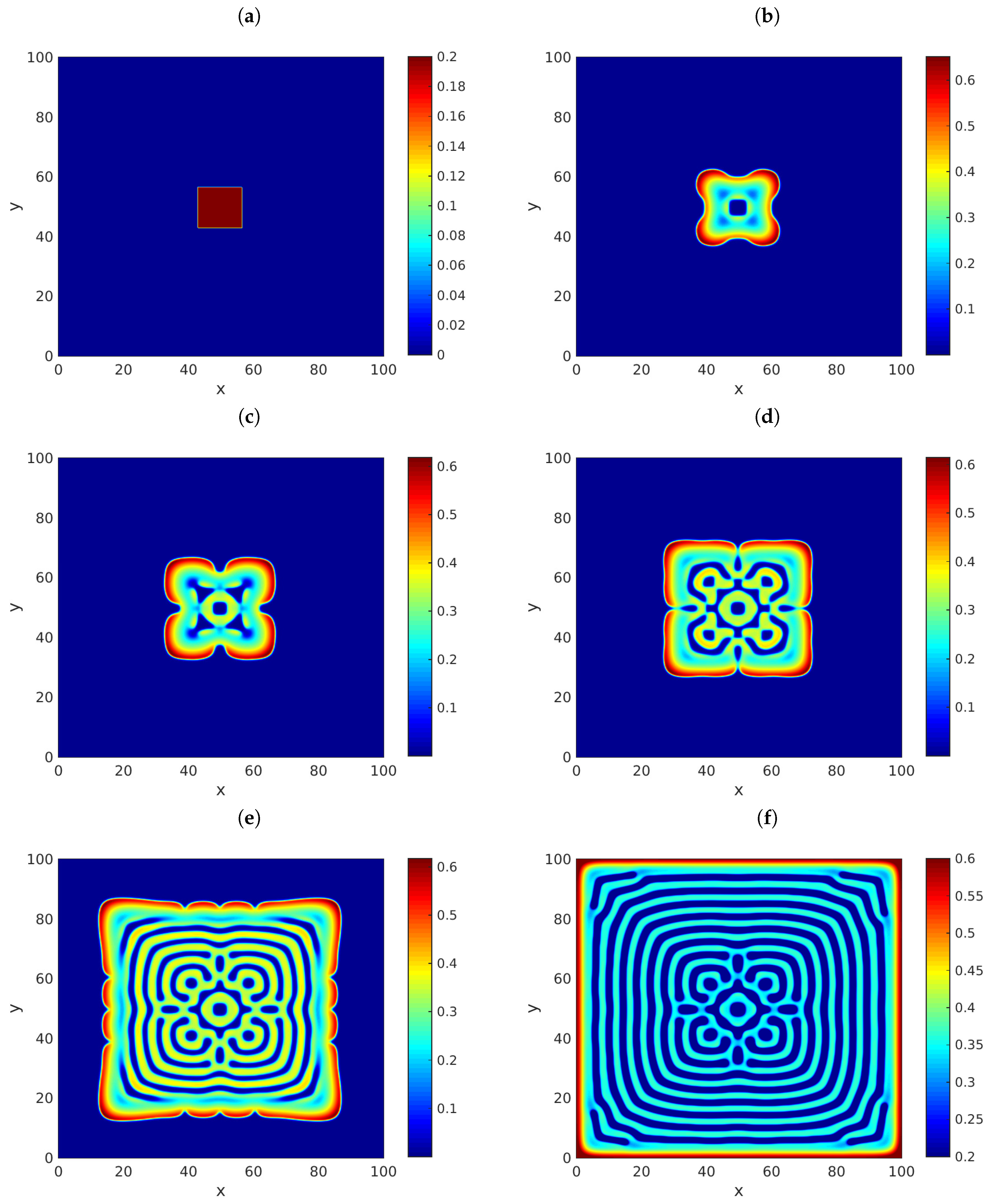
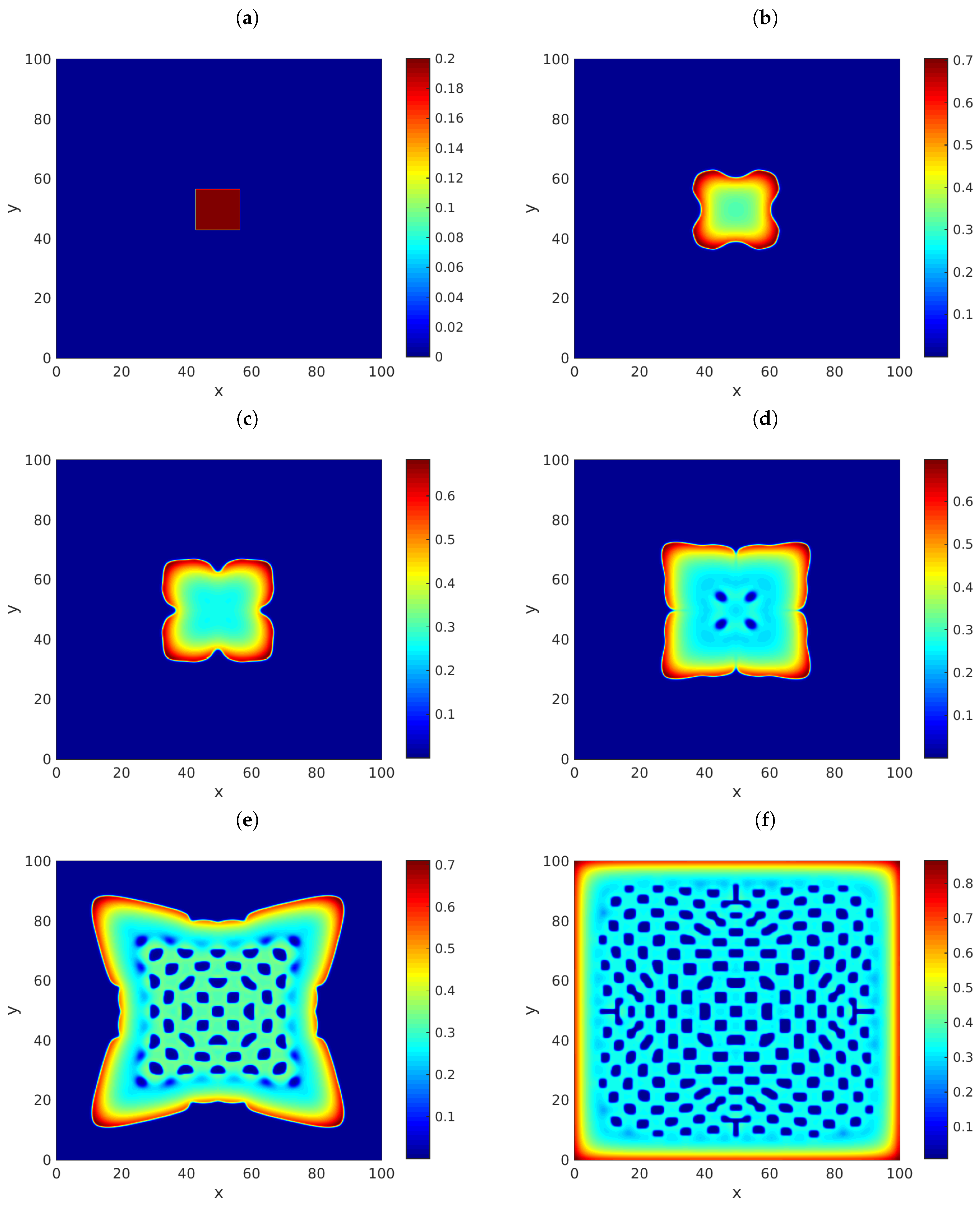
It is easy to see that this point is a stationary solution of (118), which is a model that describes the spatio-temporal dynamics of a predator–prey system without Allee effects. Obviously, this system is a particular form of the more general model (7). To approximate solutions of the present system of equations, we will let ${\varphi }_v(x)$ be any sample from a normally distributed random variable with the mean equal to $v^{\ast }$ and the standard deviation equal to $0.01$. Meanwhile, ${\varphi }_u$ will be equal to zero on all B, except on a central square at the middle of B, on which it will be constantly equal to $0.2$. Let $a=0.8$, $c=0.3$, $d=0.1$, $D_1=0.01$, and $D_2=0.6$. Figure 1 provides snapshots of the solution u in (118) at (a) $t=0$, (b) $t=160$, (c) $t=290$, (d) $t=500$, (e) $t=1010$, and (f) $t=3000$, using $\alpha =\beta =2$. The graphs exhibit the presence of complex patterns, in agreement with the results obtained in [43]. In those results, we agreed that $x=x_1$ and $y=x_2$. For illustration purposes, Figure 2 and Figure 3 provide similar results for the cases when $\alpha =\beta =1.6$ and $\alpha =\beta =1.2$, respectively. Turing patterns appear in those instances also, in spite of the fractional nature of those cases. In our simulations, we used our implementation of (20) shown in Appendix A, with $\tau =0.02$ and $h_{x_1}=h_{x_2}=1/3$. Moreover, we imposed homogeneous Neumann conditions on the boundary of B.

It is worth pointing out that the literature lacks an analytical apparatus that justifies the presence of the Turing patterns in the fractional scenarios of Figure 2 and Figure 3. In that sense, the explicit numerical methodology reported in the present paper may be a reliable tool to confirm any analytical results on the fully fractional form of (118).

In our last example, we will tackle the three-dimensional scenario. To that end, the code of Appendix A had to be adapted to the three-dimensional scenario, and parallel programming was needed in order to speed up the computer time.

Example 2.

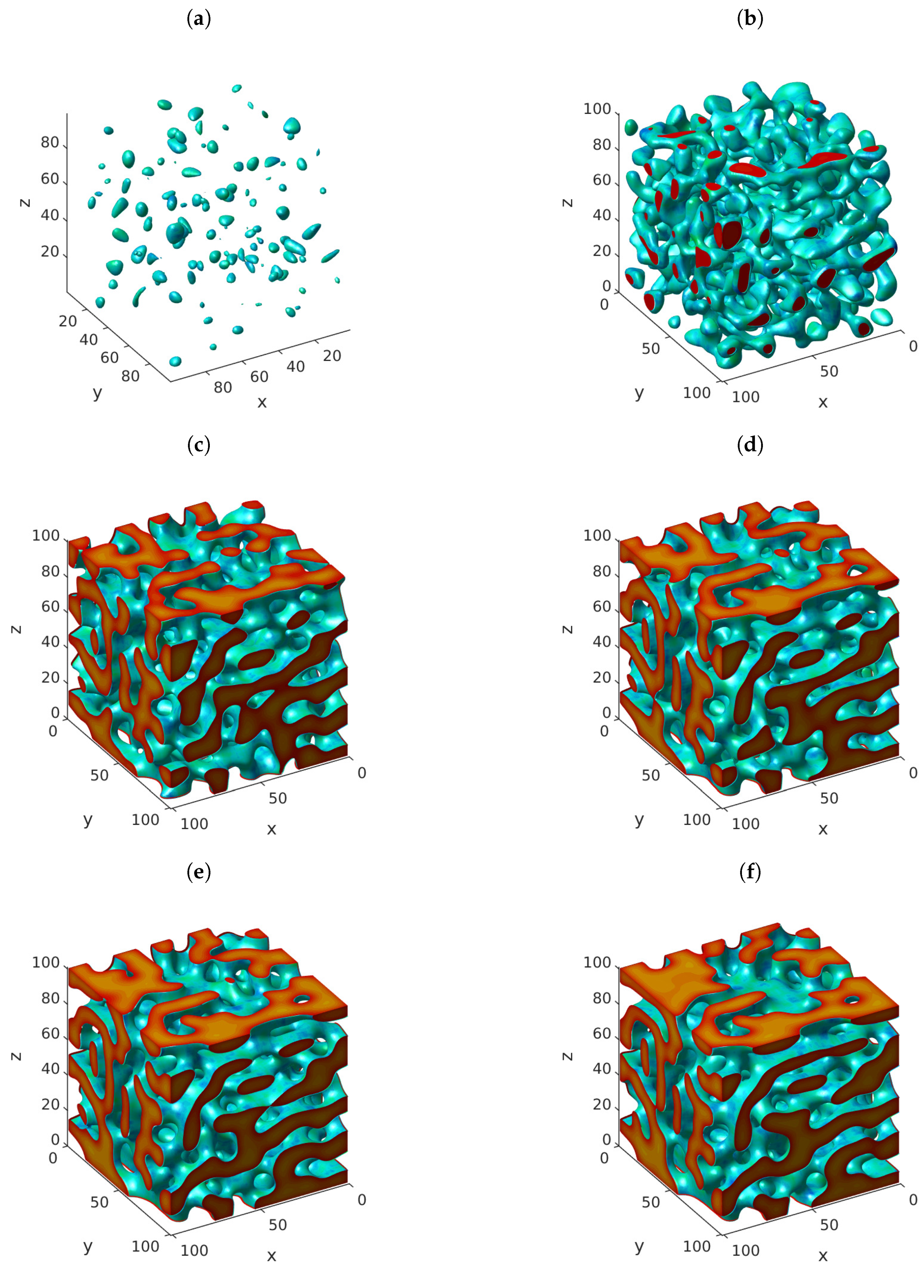
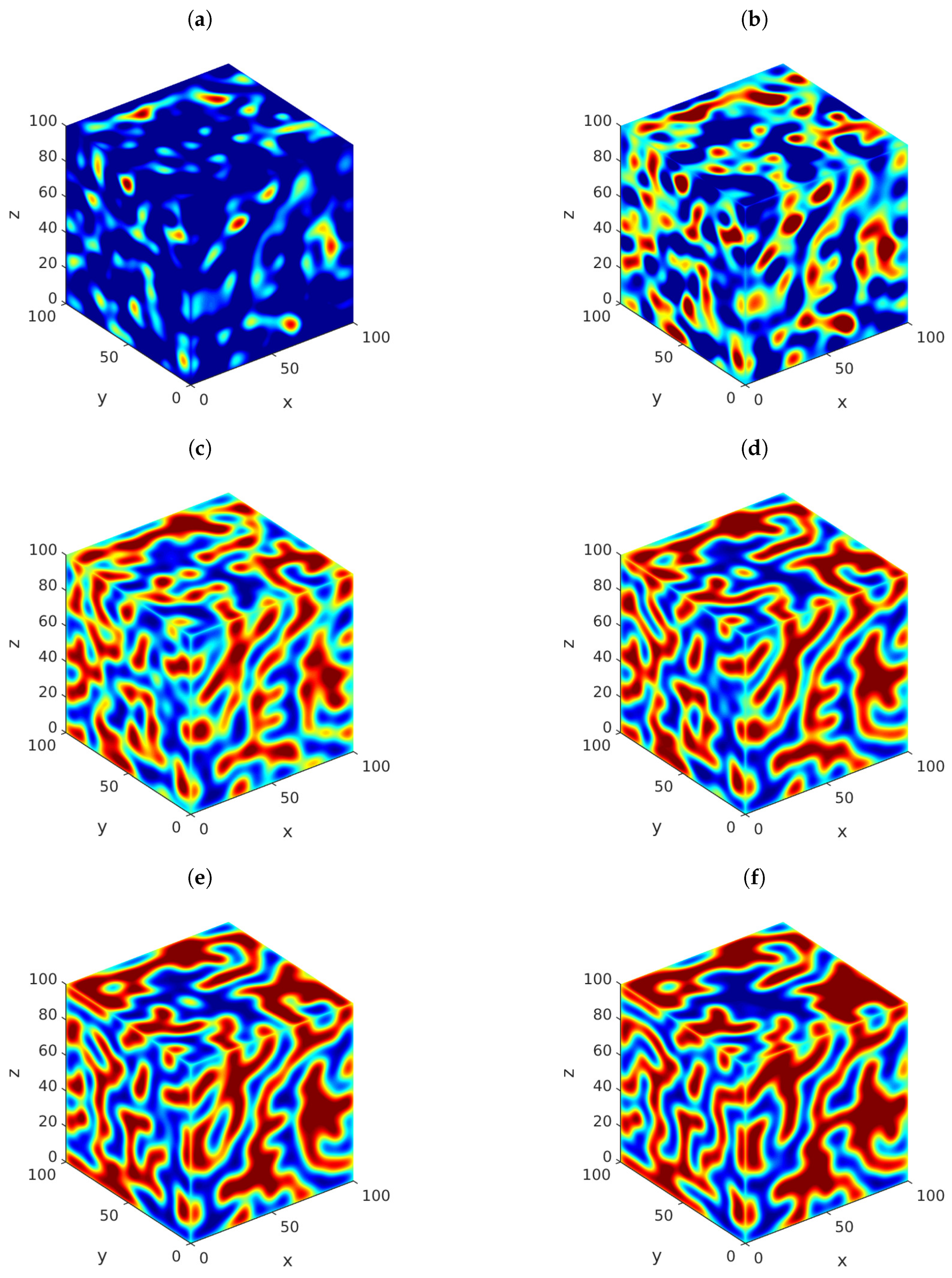
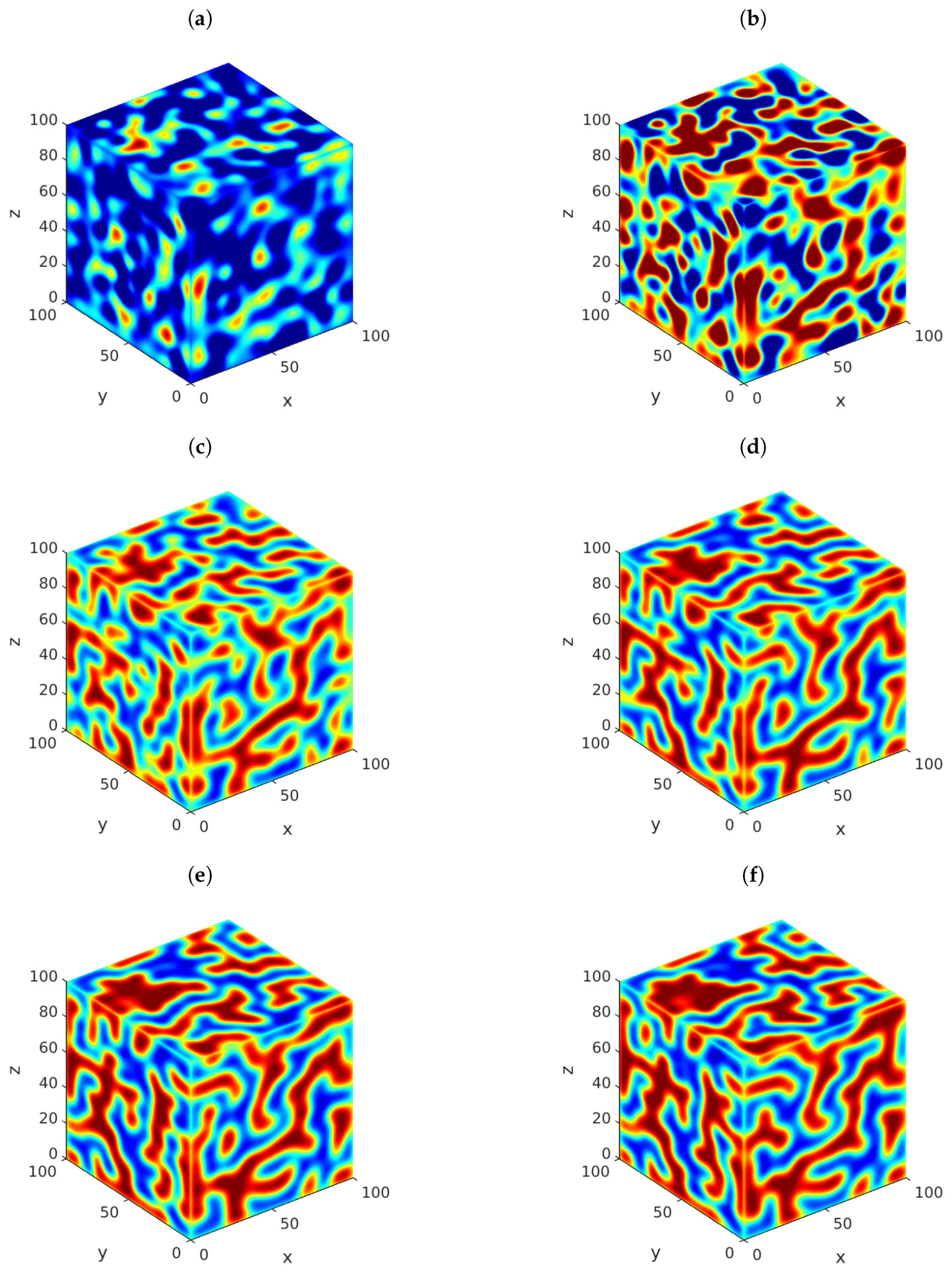
We considered the three-dimensional form of problem (118) with the same model parameters, spatial domain $\Omega =(0,100)\times (0,100)\times (0,100)\subseteq {\mathbb{R}}^3$, $\tau =0.02$, and $h_{x_1}=h_{x_2}=h_{x_3}=1$. Under these circumstances, Figure 4 shows snapshots of the solution u of the three-dimensional problem (118) at (a) $t=0$, (b) $t=160$, (c) $t=290$, (d) $t=500$, (e) $t=1010$, and (f) $t=3000$, letting $\alpha =\beta =1.6$. The graphs exhibit the presence of complex three-dimensional patterns that have not been investigated in the literature. For convenience, Figure 5 shows x-, y- and z-cross sections of the approximate solution u at the same times. In this case, the graphs exhibit the presence of two-dimensional patterns on the sides of the cube $\overline{B}$. In turn, Figure 6 and Figure 7 show similar results for the case when $\alpha =\beta =1.2$. Again, the presence of three-dimensional and two-dimensional patterns is obvious from the graphs. We performed more simulations (not included in this work to avoid redundancy) using various values of α and β. The results have shown the presence of three-dimensional complex patterns in all the cases considered.

Our last example provides numerical evidence that the emerging Turing patterns preserve their share independent of the discretization step.

Example 3.

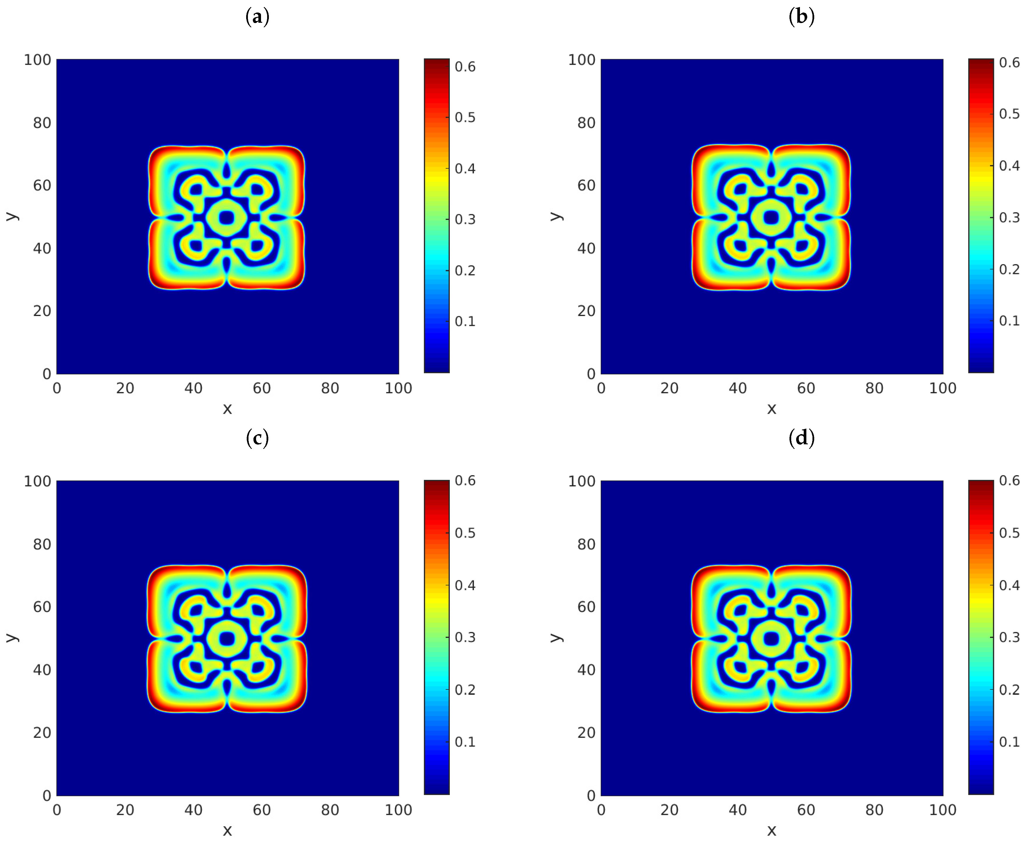
Consider the same mathematical problem of Example 1 with the model parameters$a=0.8$,$c=0.3$,$d=0.1$,$D_1=0.01$,$D_2=0.6$, and$\alpha =\beta =1.6$. Fix the temporal period$T=500$. Figure 8 shows the results of our simulations considering various values of the spatial partition norms. Throughout, we let$h=h_{x_1}=h_{x_2}$. The graphs correspond to the values (a)$h=1/3$, (b)$h=1/4$,$h=1/5$, and$h=1/8$. A similar pattern shape was obtained in all cases. These results provide numerical evidence that the type of Turing pattern is independent of the discretization spatial step-size. We performed similar experiments considering different temporal steps. The simulations are not reproduced to avoid redundancy, but they prove that the emerging patterns are also independent of τ.

7. Conclusions

In this manuscript, we studied computationally a system of two diffusive partial differential equations with coupled nonlinear reactions in generalized forms. Our system considered the presence of anomalous diffusion in multiple spatial dimensions along with suitable initial data. The model generalized various particular systems from the physical sciences, including the diffusive systems, which describe the interaction between populations of predators and preys with the Michaelis–Menten-type reaction. The system was discretized following a finite-difference approach, and two schemes were proposed to approximate the solutions. The two numerical models were rigorously analyzed to elucidate their structural and numerical properties.

As the main structural results, we established the existence and uniqueness of the numerical solutions. Moreover, we proved that the schemes were both capable of preserving the positivity and boundedness of approximations [50,51]. As in various other examples available in the literature [31,52,53,54], this was in perfect agreement with the fact that the relevant solutions of normalized population models were positive and bounded. Numerically, we proved rigorously that the schemes were consistent, stable, and convergent. Some simulations were provided in this work to illustrate the performance of the schemes. In particular, we showed the capability of one of the schemes to be applied on the investigation of Turing patterns in anomalously diffusive systems describing predator–prey interactions. To that end, a fast computational implementation in MATLAB of one of the schemes was employed. Of course, the present approach may be applied to other different scenarios [55,56].

At the closure of this manuscript, it is interesting to point out that the two discretizations of the system (7) were capable of preserving the anomalous diffusion rate. Indeed, note that those rates were equal to $D_1$ and $D_2$ for each of the partial differential equations of the continuous model (7). On the other hand, in light of Lemma 2, it follows that:

$$\begin{array}{cc}\hfill D_1\sum _{i=1}^2{\delta }_{x_i}^{(\alpha )}{u}_{m,n}^k& =D_1\left[-\frac{1}{h_{x_1}^{\alpha }}\sum _{i=0}^M{g}_{m-i}^{(\alpha )}{u}_{i,n}^k-\frac{1}{h_{x_2}^{\alpha }}\sum _{i=0}^N{g}_{n-i}^{(\alpha )}{u}_{m,i}^k\right]\hfill \\ & =D_1\left[\frac{{\partial }^{\alpha }u(x_{1,m},x_{2,n},t_k)}{\partial |x_1{|}^{\alpha }}+\frac{{\partial }^{\alpha }u(x_{1,m},x_{2,n},t_k)}{\partial |x_2{|}^{\alpha }}\right]+\mathcal{O}(h_{x_1}^2)+\mathcal{O}(h_{x_2}^2)\hfill \\ & =D_1\sum _{i=1}^2\frac{{\partial }^{\alpha }u(x_{1,m},x_{2,n},t_k)}{\partial |x_i{|}^{\alpha }}+{\mathcal{O}(\parallel h\parallel }^2).\hfill \end{array}$$

(120)

Similarly, it is easy to check that:

$$D_2\sum _{i=1}^2{\delta }_{x_i}^{(\beta )}{v}_{m,n}^k=D_2\sum _{i=1}^2\frac{{\partial }^{\beta }v(x_{1,m},x_{2,n},t_k)}{\partial |x_i{|}^{\beta }}+{\mathcal{O}(\parallel h\parallel }^2).$$

(121)

It follows that our spatial discretizations are capable of preserving the anomalous diffusion rate.

References

Xiao, Y.; Chen, L. Modeling and analysis of a predator–prey model with disease in the prey. Math. Biosci.2001, 171, 59–82. [Google Scholar] [CrossRef]
Ji, C.; Jiang, D.; Shi, N. Analysis of a predator–prey model with modified Leslie–Gower and Holling-type II schemes with stochastic perturbation. J. Math. Anal. Appl.2009, 359, 482–498. [Google Scholar] [CrossRef]
Deng, H.; Chen, F.; Zhu, Z.; Li, Z. Dynamic behaviors of Lotka–Volterra predator–prey model incorporating predator cannibalism. Adv. Differ. Equ.2019, 2019, 1–17. [Google Scholar] [CrossRef]
Song, Q.; Yang, R.; Zhang, C.; Tang, L. Bifurcation analysis in a diffusive predator–prey system with Michaelis–Menten-type predator harvesting. Adv. Differ. Equ.2018, 2018, 329. [Google Scholar] [CrossRef]
Balagaddé, F.K.; Song, H.; Ozaki, J.; Collins, C.H.; Barnet, M.; Arnold, F.H.; Quake, S.R.; You, L. A synthetic Escherichia coli predator–prey ecosystem. Mol. Syst. Biol.2008, 4, 187. [Google Scholar] [CrossRef]
Gourley, S.A.; Kuang, Y. A stage structured predator–prey model and its dependence on maturation delay and death rate. J. Math. Biol.2004, 49, 188–200. [Google Scholar] [CrossRef]
Wang, L.L.; Li, W.T. Periodic solutions and permanence for a delayed nonautonomous ratio-dependent predator–prey model with Holling type functional response. J. Comput. Appl. Math.2004, 162, 341–357. [Google Scholar] [CrossRef]
Banerjee, M.; Mukherjee, N.; Volpert, V. Prey-predator model with a nonlocal bistable dynamics of prey. Mathematics2018, 6, 41. [Google Scholar] [CrossRef]
Yousef, A.; Yousef, F.B. Bifurcation and Stability Analysis of a System of Fractional-Order Differential Equations for a Plant–Herbivore Model with Allee Effect. Mathematics2019, 7, 454. [Google Scholar] [CrossRef]
Shabbir, M.S.; Din, Q.; Safeer, M.; Khan, M.A.; Ahmad, K. A dynamically consistent nonstandard finite difference scheme for a predator–prey model. Adv. Differ. Equ.2019, 2019, 1–17. [Google Scholar] [CrossRef]
Dimitrov, D.T.; Kojouharov, H.V. Positive and elementary stable nonstandard numerical methods with applications to predator–prey models. J. Comput. Appl. Math.2006, 189, 98–108. [Google Scholar] [CrossRef]
Nindjin, A.; Aziz-Alaoui, M.; Cadivel, M. Analysis of a predator–prey model with modified Leslie–Gower and Holling-type II schemes with time delay. Nonlinear Anal. Real World Appl.2006, 7, 1104–1118. [Google Scholar] [CrossRef]
Dimitrov, D.T.; Kojouharov, H.V. Nonstandard finite-difference methods for predator–prey models with general functional response. Math. Comput. Simul.2008, 78, 1–11. [Google Scholar] [CrossRef]
Yu, Y.; Deng, W.; Wu, Y. Positivity and boundedness preserving schemes for space–time fractional predator–prey reaction–diffusion model. Comput. Math. Appl.2015, 69, 743–759. [Google Scholar] [CrossRef]
Kochubei, A.N.; Kondratiev, Y. Growth Equation of the General Fractional Calculus. Mathematics2019, 7, 615. [Google Scholar] [CrossRef]
Macías-Díaz, J.E. Persistence of nonlinear hysteresis in fractional models of Josephson transmission lines. Commun. Nonlinear Sci. Numer. Simul.2017, 53, 31–43. [Google Scholar] [CrossRef]
Macías-Díaz, J.E. Numerical simulation of the nonlinear dynamics of harmonically driven Riesz-fractional extensions of the Fermi–Pasta–Ulam chains. Commun. Nonlinear Sci. Numer. Simul.2018, 55, 248–264. [Google Scholar] [CrossRef]
Koeller, R. Applications of fractional calculus to the theory of viscoelasticity. ASME Trans. J. Appl. Mech.1984, 51, 299–307. [Google Scholar] [CrossRef]
Povstenko, Y. Theory of thermoelasticity based on the space-time-fractional heat conduction equation. Phys. Scr.2009, 2009, 014017. [Google Scholar] [CrossRef]
Scalas, E.; Gorenflo, R.; Mainardi, F. Fractional calculus and continuous-time finance. Phys. A Stat. Mech. Its Appl.2000, 284, 376–384. [Google Scholar] [CrossRef]
Glöckle, W.G.; Nonnenmacher, T.F. A fractional calculus approach to self-similar protein dynamics. Biophys. J.1995, 68, 46–53. [Google Scholar] [CrossRef]
Namias, V. The fractional order Fourier transform and its application to quantum mechanics. IMA J. Appl. Math.1980, 25, 241–265. [Google Scholar] [CrossRef]
Singh, J.; Kumar, D.; Baleanu, D. On the analysis of fractional diabetes model with exponential law. Adv. Differ. Equ.2018, 2018, 231. [Google Scholar] [CrossRef]
Yusuf, A.; Aliyu, A.I.; Baleanu, D. Conservation laws, soliton-like and stability analysis for the time fractional dispersive long-wave equation. Adv. Differ. Equ.2018, 2018, 319. [Google Scholar] [CrossRef]
Ghanbari, B.; Yusuf, A.; Baleanu, D. The new exact solitary wave solutions and stability analysis for the (2+1) (2+1)-dimensional Zakharov–Kuznetsov equation. Adv. Differ. Equ.2019, 2019, 49. [Google Scholar] [CrossRef]
Li, H.L.; Muhammadhaji, A.; Zhang, L.; Teng, Z. Stability analysis of a fractional-order predator–prey model incorporating a constant prey refuge and feedback control. Adv. Differ. Equ.2018, 2018, 325. [Google Scholar] [CrossRef]
Huang, C.; Cao, J.; Xiao, M.; Alsaedi, A.; Alsaadi, F.E. Controlling bifurcation in a delayed fractional predator–prey system with incommensurate orders. Appl. Math. Comput.2017, 293, 293–310. [Google Scholar] [CrossRef]
Wang, J.; Cheng, H.; Liu, H.; Wang, Y. Periodic solution and control optimization of a prey-predator model with two types of harvesting. Adv. Differ. Equ.2018, 2018, 41. [Google Scholar] [CrossRef]
Rihan, F.; Lakshmanan, S.; Hashish, A.; Rakkiyappan, R.; Ahmed, E. Fractional-order delayed predator–prey systems with Holling type-II functional response. Nonlinear Dyn.2015, 80, 777–789. [Google Scholar] [CrossRef]
Macías-Díaz, J.E. Sufficient conditions for the preservation of the boundedness in a numerical method for a physical model with transport memory and nonlinear damping. Comput. Phys. Commun.2011, 182, 2471–2478. [Google Scholar] [CrossRef]
Macías-Díaz, J.E. An explicit dissipation-preserving method for Riesz space-fractional nonlinear wave equations in multiple dimensions. Commun. Nonlinear Sci. Numer. Simul.2018, 59, 67–87. [Google Scholar] [CrossRef]
Alikhanov, A.A. A new difference scheme for the time fractional diffusion equation. J. Comput. Phys.2015, 280, 424–438. [Google Scholar] [CrossRef]
Bhrawy, A.H.; Abdelkawy, M.A. A fully spectral collocation approximation for multi-dimensional fractional Schrödinger equations. J. Comput. Phys.2015, 294, 462–483. [Google Scholar] [CrossRef]
El-Ajou, A.; Arqub, O.A.; Momani, S. Approximate analytical solution of the nonlinear fractional KdV–Burgers equation: A new iterative algorithm. J. Comput. Phys.2015, 293, 81–95. [Google Scholar] [CrossRef]
Liu, F.; Zhuang, P.; Turner, I.; Anh, V.; Burrage, K. A semi-alternating direction method for a 2-D fractional FitzHugh–Nagumo monodomain model on an approximate irregular domain. J. Comput. Phys.2015, 293, 252–263. [Google Scholar] [CrossRef]
Chen, B. The influence of commensalism on a Lotka–Volterra commensal symbiosis model with Michaelis–Menten type harvesting. Adv. Differ. Equ.2019, 2019, 43. [Google Scholar] [CrossRef]
Tarasov, V.E. Partial fractional derivatives of Riesz type and nonlinear fractional differential equations. Nonlinear Dyn.2016, 86, 1745–1759. [Google Scholar] [CrossRef]
Tarasov, V.E. Continuous limit of discrete systems with long-range interaction. J. Phys. A Math. Gen.2006, 39, 14895. [Google Scholar] [CrossRef]
Ortigueira, M.D. Riesz potential operators and inverses via fractional centred derivatives. Int. J. Math. Math. Sci.2006, 2006. [Google Scholar] [CrossRef]
Podlubny, I. Fractional Differential Equations: An Introduction to Fractional Derivatives, Fractional Differential Equations, to Methods of Their Solution and Some of Their Applications; Elsevier: Amsterdam, The Netherlands, 1998; Volume 198. [Google Scholar]
Rao, F.; Kang, Y. The complex dynamics of a diffusive prey–predator model with an Allee effect in prey. Ecol. Complex.2016, 28, 123–144. [Google Scholar] [CrossRef]
Wang, X.; Liu, F.; Chen, X. Novel second-order accurate implicit numerical methods for the Riesz space distributed-order advection-dispersion equations. Adv. Math. Phys.2015. [Google Scholar] [CrossRef]
Plemmons, R.J. M-matrix characterizations. I—Nonsingular M-matrices. Linear Algebra Its Appl.1977, 18, 175–188. [Google Scholar] [CrossRef]
Tian, G.X.; Huang, T.Z. Inequalities for the minimum eigenvalue of M-matrices. ELA Electron. J. Linear Algebra2010, 20, 21. [Google Scholar] [CrossRef]
Chen, S.; Liu, F.; Turner, I.; Anh, V. An implicit numerical method for the two-dimensional fractional percolation equation. Appl. Math. Comput.2013, 219, 4322–4331. [Google Scholar] [CrossRef]
Cutolo, A.; Piccoli, B.; Rarità, L. An upwind-Euler scheme for an ODE-PDE model of supply chains. SIAM J. Sci. Comput.2011, 33, 1669–1688. [Google Scholar] [CrossRef][Green Version]
Cascone, A.; Marigo, A.; Piccoli, B.; Rarità, L. Decentralized optimal routing for packets flow on data networks. Discret. Contin. Dyn. Syst. Ser. B (DCDS-B)2010, 13, 59–78. [Google Scholar]
Ervin, V.; Macías-Díaz, J.; Ruiz-Ramírez, J. A positive and bounded finite element approximation of the generalized Burgers–Huxley equation. J. Math. Anal. Appl.2015, 424, 1143–1160. [Google Scholar] [CrossRef]
Macías-Díaz, J.E.; Villa-Morales, J. A deterministic model for the distribution of the stopping time in a stochastic equation and its numerical solution. J. Comput. Appl. Math.2017, 318, 93–106. [Google Scholar] [CrossRef]
Morales-Hernández, M.D.; Medina-Ramírez, I.E.; Avelar-González, F.J.; Macías-Díaz, J.E. An efficient recursive algorithm in the computational simulation of the bounded growth of biological films. Int. J. Comput. Methods2012, 9, 1250050. [Google Scholar] [CrossRef]
Macías-Díaz, J.E.; Puri, A. A boundedness-preserving finite-difference scheme for a damped nonlinear wave equation. Appl. Numer. Math.2010, 60, 934–948. [Google Scholar] [CrossRef]
Macías-Díaz, J.E.; Puri, A. An explicit positivity-preserving finite-difference scheme for the classical Fisher–Kolmogorov–Petrovsky–Piscounov equation. Appl. Math. Comput.2012, 218, 5829–5837. [Google Scholar] [CrossRef]
Cascone, A.; D’Apice, C.; Piccoli, B.; Rarità, L. Circulation of car traffic in congested urban areas. Commun. Math. Sci.2008, 6, 765–784. [Google Scholar] [CrossRef]
Manzo, R.; Piccoli, B.; Rarita, L. Optimal distribution of traffic flows in emergency cases. Eur. J. Appl. Math.2012, 23, 515–535. [Google Scholar] [CrossRef]
Figure 1.
Snapshots of the approximate solution u in (118) versus x and y. The parameters employed are , , , , , and . Meanwhile, we considered the times (a) , (b) , (c) , (d) , (e) , and (f) . We let be a random sample from a normally distributed random variable with the mean equal to and the standard deviation equal to , and is the function depicted in (a). The approximations were calculated using our implementation of (20) shown in Appendix A, with and .
Figure 2.
Figure 3.
Figure 4.
Snapshots of the approximate solution u in (118) versus x, y, and z. The parameters employed are , , , , , and . Meanwhile, we considered the times (a) , (b) , (c) , (d) , (e) , and (f) . The initial data are random samples of a uniform distribution on . The approximations were calculated using our implementation of (20), with and .
Figure 5.
Snapshots of x-, y-, and z-cross-sections of the approximate solution u of (118) versus x, y, and z. The parameters employed are , , , , , and . Meanwhile, we considered the times (a) , (b) , (c) , (d) , (e) , and (f) . The initial data are random samples of a uniform distribution on . The approximations were calculated using our implementation of (20), with and .
Figure 6.
Snapshots of the approximate solution u of (118) versus x, y, and z. The parameters employed are , , , , , and . Meanwhile, we considered the times (a) , (b) , (c) , (d) , (e) , and (f) . The initial data are random samples of a uniform distribution on . The approximations were calculated using our implementation of (20), with and .
Figure 7.
Figure 8.
Snapshots of the approximate solution u in (118) versus x and y, at the time . The parameters employed are , , , , , and . We let be a random sample from a normally distributed random variable with the mean equal to and the standard deviation equal to , and is the function depicted in (a). The approximations were calculated using our implementation of (20) shown in Appendix A, with and satisfying (a) , (b) , (c) , and (d) .
Alba-Pérez, J.; Macías-Díaz, J.E.