Article

Enhancement of Deep Learning in Image Classification Performance Using Xception with the Swish Activation Function for Colorectal Polyp Preliminary Screening

1
Department of Tropical Agriculture and International Cooperation, National Pingtung University of Science and Technology, Pingtung 912, Taiwan
2
Department of Management Information Systems, National Pingtung University of Science and Technology, Pingtung 912, Taiwan
3
Department of Biochemistry and Molecular Biology, National Cheng Kung University, Tainan 701, Taiwan
4
Center for Prognosis Research, School of Primary, Community and Social Care, Keele University, Keele ST5 5BG, UK
*
Author to whom correspondence should be addressed.
Mathematics 2019, 7(12), 1170; https://doi.org/10.3390/math7121170
Submission received: 14 October 2019 / Revised: 15 November 2019 / Accepted: 20 November 2019 / Published: 3 December 2019
(This article belongs to the Special Issue Recent Advances in Deep Learning)

Abstract

:
One of the leading forms of cancer is colorectal cancer (CRC), which is responsible for increasing mortality in young people. The aim of this paper is to provide an experimental modification of deep learning of Xception with Swish and assess the possibility of developing a preliminary colorectal polyp screening system by training the proposed model with a colorectal topogram dataset in two and three classes. The results indicate that the proposed model can enhance the original convolutional neural network model with evaluation classification performance by achieving accuracy of up to 98.99% for classifying into two classes and 91.48% for three classes. For testing of the model with another external image, the proposed method can also improve the prediction compared to the traditional method, with 99.63% accuracy for true prediction of two classes and 80.95% accuracy for true prediction of three classes.

1. Introduction

Colorectal cancer (CRC) is a form of cancer that occurs globally and is one of the most common forms of cancer among both men and women in terms of the causes of human mortality [1,2]. Recently, reports have identified that the number of people with CRC younger than 50 years old is increasing, which means cancer screening is a more essential process than ever [3,4]. Cancer features unlimited division and appears in living anomalous cells in various organs, as well as when abnormal cells appear and grow in the colon, which is the case with CRC [4]. The beginning of CRC involves 70% growth from adenomatous polyps, which can develop inside the colon lining. It grows slowly over a period of approximately 10 to 20 years [4,5,6]. Evaluation of CRC diagnosis is critical [4] because the survival rate is increased by timely detection, which is considered a significant process in cancer diagnosis. The main tools for diagnosis include medical imaging [1], which can realistically display patients’ internal organs in order to enable more rapid screening and diagnosis by health care experts for continued planning and subsequent treatment procedures [7].
Topograms are 2D overview images obtained from a tomographic machine. Topogram images are generated for screening and planning before advancing to the next procedural step, such as computer tomography (CT) scanning [7]. These kinds of medical images easily and conveniently capture anterior, posterior, and lateral views of patients’ bodies [7,8]. With an identical process of colorectal polyp identification, colonography utilizes a scanning machine to acquire an overview image of the colorectal area to identify abnormalities of polyps so they can be removed before developing or spreading into severe cancer [9]. However, the diagnostic process has several limitations, including that manual interpretation of medical images can be tedious, require a lot of time, and be subject to bias and human error [1]. Medical imaging involves digital images that can be used for analysis by a computer. Therefore, image analysis based on computer-aided diagnosis (CAD) systems for medical image classification is essential in disease detection, screening, and diagnosis [10]. Applying computer-aided screening for colorectal polyp classification and screening with multimedia summarization techniques [11,12] has advantages in increasing the capability of diagnosing colorectal polyps [13]. Figure 1 illustrates the preliminary screening system concept for colonoscopy diagnosis to help physicians’ inspections. This screening system can be helpful for preliminary classification of colorectal topogram images, which can be used to plan the next step in diagnosis.
Deep learning has been popularly used since 1998 [14], when an early deep learning method named LeNet was created with a convolutional neural network (CNN) for recognizing digitized handwriting. In 2006 [15], deep learning became more powerful with fine-tuning, and was used to generate a better model of digitized handwritten image classification than the discriminative learning technique. Dimensionality reduction by adopting deep learning is also described in [16]. The proposed method was an improvement compared to the traditional method of principal component analysis (PCA). More recently, deep learning in the development of CNN architecture has been joined with image classification by ImageNet [17]. Since then, there has been development and application of deep learning in various fields, including in medical processes. Deep learning can assist health care experts by requiring less time for the screening process and improving the efficiency of diagnosis [10]. The deep learning technique, especially in terms of CNN, has become widely applied in a variety of medical procedures, such as medical image reconstruction [18], clinical report classification [19], diagnosis [20], identification of disease [21], cancer detection [22], disease screening [23], and medical image classification [24]. The success of CNN has increased in medical image analysis [25], especially for colorectal polyp diagnostic procedures [26,27]. Several studies applied CNN as a solution for problems in medical images with CRC and colorectal polyps. Some studies used CNN for segmentation with magnetic resonance imaging (MRI), such as [28], in which the combination of 3D CNN and 3D level-set for automated segmentation of colorectal cancer yielded segmentation accuracy of 93.78%. In addition, [29] proposed a CNN with hybrid loss for automatic colorectal cancer segmentation and outperformed with an average surface distance of 3.83 mm and mean Dice similarity coefficient (DSC) of 0.721.
For CT imaging [30], applications of CNN by transfer learning for electronic cleansing may improve accuracy from 89% to 94% for visualization of colorectal polyp images. Furthermore, the CNN developed by [31] showed improved colorectal polyp classification performance by area under the curve (AUC) of 86 and accuracy of 83% on CT image datasets.
Several studies focused on endoscopic image datasets, such as [32], which developed a CNN for detecting polyps in real time and validating a new colonoscopy image collection with detected polyps, obtaining AUC of 0.984%, sensitivity of 94.38%, and specificity of 95.92%. [33] Creating a CNN for polyp detection enabled precise detection at 88.6% and recall at 71.6%. A polyp segmentation method with full CNN for different sizes and shapes of colorectal polyps used as ground truth images for evaluation was developed in [34]. Segmentation accuracy of 97.77% was achieved. A CNN for real-time evaluation of endoscopic videos was proposed in [35] to identify colorectal polyps, with achieved accuracy of 94%. Modified region-based CNN training on wireless capsule endoscopy images in [36] provided detection performance precision of 98.46%, recall of 95.52%, F1 score of 96.67%, and F2 score of 96.10%.
Utilizing tissue image datasets, [2] developed an experimental CNN with transfer learning and fine-tuning for histology in CRC diagnosis, in which the CNN provided good testing classification accuracy up to 90%. In [37], large image sizes were applied with CNN and evaluated for colorectal cancer grading classification, achieving accuracy for two classes of 99.28% and three classes of 95.70%. In [38], a CNN was trained by transfer learning, with achieved accuracy of 94.3% using an external testing dataset in nine classes. Many of the above studies obviously showed that CNN can be used for colorectal polyp classification in the context of screening to generate highly accurate and excellent results when using different kinds of medical image datasets, including MR, CT, tissue, and endoscopic images. However, a CNN method has not yet been utilized with colorectal topogram images, which could possibly be used to assist physicians in preliminary screening and rapid diagnosis.
There have been many improvements of CNN architecture since 2012. The classic architecture, called AlexNet [39], demonstrated essential improvements over the previous architecture for image classification. More recently, several CNN architectures have been developed to enhance image classification performance, such as in VGGNet in 2014 [40], GoogleNet, also known as Inception [41], and ResNet [42], established in 2015. These CNN architectures were developed under six main improvements: convolutional layer, pooling layer, activation function, loss function, regularization, and optimization [43]. In 2017, Extreme Inception, also known as Xception, was developed, a version in the Inception family from the Xception architecture developed by Chollet [44] at Google. The Xception architecture concept is based on the Inception module [41], with modifications and a combination of convolutional layers, inception modules, depth-wise separable convolutions, and residual connections to improve CNN performance. The results of Xception indicate that classification performance was improved compared to VGGNet, ResNet, and Inception v3 [45]. The original Xception architecture used rectified linear unit (ReLU) [46] for the activation function. The recent activation function, named Swish [47], can enhance the image classification accuracy of NASNet-Mobile (established in 2018) [48] and InceptionResNet v2 (released in 2016) [49]. There has not been a study on the application of Swish with Xception. Replacing the ReLU with Swish [47] inside Xception may enhance the classification performance compared to the original Xception and other CNN architectures.
The purpose of this study is to provide a novel modification of Xception by applying the Swish activation function to determine the possibility of developing a preliminary screening system for colorectal polyps, by training our proposed Xception with Swish model with a colonography topogram image dataset. The proposed system screens colorectal polyps into two classes: found and not found. In addition, we also classify polyps in three categories: small size, large size, and not found. Moreover, we compare the results with the original Xception architecture and other established modern CNN architectures that are also modified with Swish, and the performance of Xception with Swish indicates excellent results compared to other CNN methods.
The remainder of the paper is structured as follows: the Xception architecture, Swish activation function, and modification of Xception with Swish for preliminary screening of colorectal polyps are described in Section 2. In Section 3, we provide the materials and methods, including topogram image dataset, image augmentation method, specification of hardware and software, programming language, and colorectal polyp classification method, and compare the experimental results. Section 4 presents more details on the experimental results and a discussion of the image classification models in the context of a preliminary colorectal polyp screening system. The conclusion of this study is presented in Section 5.

2. Xception Architecture, Swish Activation Function, and Model Modification

The continuous development of deep learning of CNN has improved the architecture for more accurate image classification techniques. Similarly, Xception architecture was developed under several important concepts, including convolutional layer, depth-wise separable convolution layer, inception module, and residual connections. Also, CNN architecture for the activation function is necessary, in which Swish is a new activation function created to improve the traditional activation function. This section proposes the theoretical Xception architecture, as well as the Swish activation function and a new modification of the Xception with Swish image classification model for preliminary colorectal polyp screening.

2.1. Xception Architecture

Xception [44] is defined as a hypothesis based on the Inception module, which creates correlations of cross-channels and spatial relations within feature maps of CNN able to be completely decoupled. Figure 2a illustrates the general Inception module [41] from Inception v3 [45], the module using cross-channel correlations by separating the input data in four ways to convolution size of 1 × 1 and average pooling, then maps correlations via convolution size of 3 × 3 and forwards them for concatenation. According to Inception, the idea is transformed to the Xception module, as shown in Figure 2b. After input, data using only one size of 1 × 1 convolution create separate convolution sizes of 3 × 3 without average pooling, which proceed in nonoverlapping sections of the output channels to then be fed forward for concatenation. The Xception module is robust, stronger than the Inception module, and can operate correlations of cross-channels and spatial relations with maps fully decoupled.
After obtaining the notion of the Xception module, the previous theory of depth-wise separable convolution is used to design the neural network [44] and major composition inside the Xception architecture, as described below.

2.1.1. Convolutional Layer

In applying convolutional layers inside the Xception architecture, there is layer after the input layer, generating convolutional kernels to calculate different feature maps to show the features of the input data. The new feature map will be collected by a first convolution operation with detection results from convolutional kernels, which then feed the result to the calculation of the activation function. To produce each feature map, the convolution kernels are divided into all areas of the input data. The different convolution kernels create the absolute results of the feature maps; mathematically, the position (i, j) upon feature value in the feature map as the kth layer determines the lth, computed as
S i , j , k l = W v k l C i , j l + B v k l
where the weight vector is defined as W v k l and B v k l , set for the bias value of the kth filter of the lth layer, for C i , j l as the center of input patch on (i, j) position of the lth layer. In sharing the feature map of S i , j , k l , it creates the calculation of the W v k l kernel. The advantages of the weight sharing process include reducing complications and improving the network for effortless training of the model. Every convolutional layer of Xception will be inserted with batch normalization [50] and the activation function, and the original activation function is ReLU in the following equation:
R e L U ( d ) = m a x ( d , 0 )
where d represents the input data. It is linear for all positive values and zero for all negative values. ReLU is not complex math with nonlinearity of the network, which is essential in CNN for identifying the nonlinear features that make faster convergences and better predictions, with less overfitting.

2.1.2. Depth-Wise Separable Convolution Layer

The significant layers of Xception are the depth-wise separable convolutions. These can reduce the computation and model parameters, which are organized in the spatial dimensions and depth dimensions of color channels. This is done by dividing from the traditional convolution process more deeply with depth-wise convolution linked to point-wise convolution [51] by creating a convolution kernel size of 1 × 1, which operates the depth-wise separable convolution illustrated in Figure 3. The depth-wise convolution generates a filter to each channel of input data set to M, and produces the feature map to determine D F × D F × M and depth-wise convolution using one filter of the input channel computed by the following equation:
G ^ k , p , m = i , j , m K ^ i , j , m × F k + i 1 , p + j 1 , m
where G ^ substitutes the output of feature maps generated by F, which is the feature map input. K ^ indicates the depth-wise convolution kernel size of D k × D k × M. The mth filter in K ^ is utilized to channel the mth in F for an estimate of the feature map output. The pixel position of the convolution kernel imposes to i, j and the pixel position of the feature map defines k, p.
Figure 3 shows that the three color channels of red, blue, and green (RBG) are collected by a separation of the depth-wise convolution 3 × 3 filters. After the convolution operation, an image appears in multiple channels and the image can be interpreted in every color channel. Then, the point-wise convolution by learning of 1 × 1 convolution filters give the output to forward to the next layer operation. For Xception, after the depth-wise separable convolution layer utilizes batch normalization, the next layers employ the max-pooling layer to reduce the cost of computation and help to interpret invariance by assigning an equation as
F m = M a x P o o l i n g ( F i , v )
where v assigns the filter of max-pooling. The output feature map defines F m , which is arranged in shape size, where each F m stores the maximal value of F i in the input feature map.

2.1.3. Residual Connection

The residual connection was established under another CNN architecture called ResNet [40], in which the internal network applies identity shortcut connections directly to the latest layers. The residual block determines the parameters as P i , which can be written in a function as
O v = f ( I v , { P i } ) + I v
where Iv represents the input vectors and Ov the output vectors of the layers. The calculation of f(Iv, { P i }) gives the residual mapping to be learned. The advantage of residual connection is that it can prevent signal extenuation by the transformation of multiple stacked nonlinearities. It is also faster for training the model. The residual shortcut connection of ResNet is shown in Figure 4a, and an example of adopting Xception is shown in Figure 4b.
Figure 4a shows that the input of X can direct a late layer by a shortcut of identity blocks. Figure 4b demonstrates applying the shortcut of residual connection directly to a late layer via 1 × 1 convolution operation with a step of 2 × 2. All of the main components above the convolutional layer, activation function, depth-wise separable convolution layer, max-pooling layer, and residual connection can be assembled.
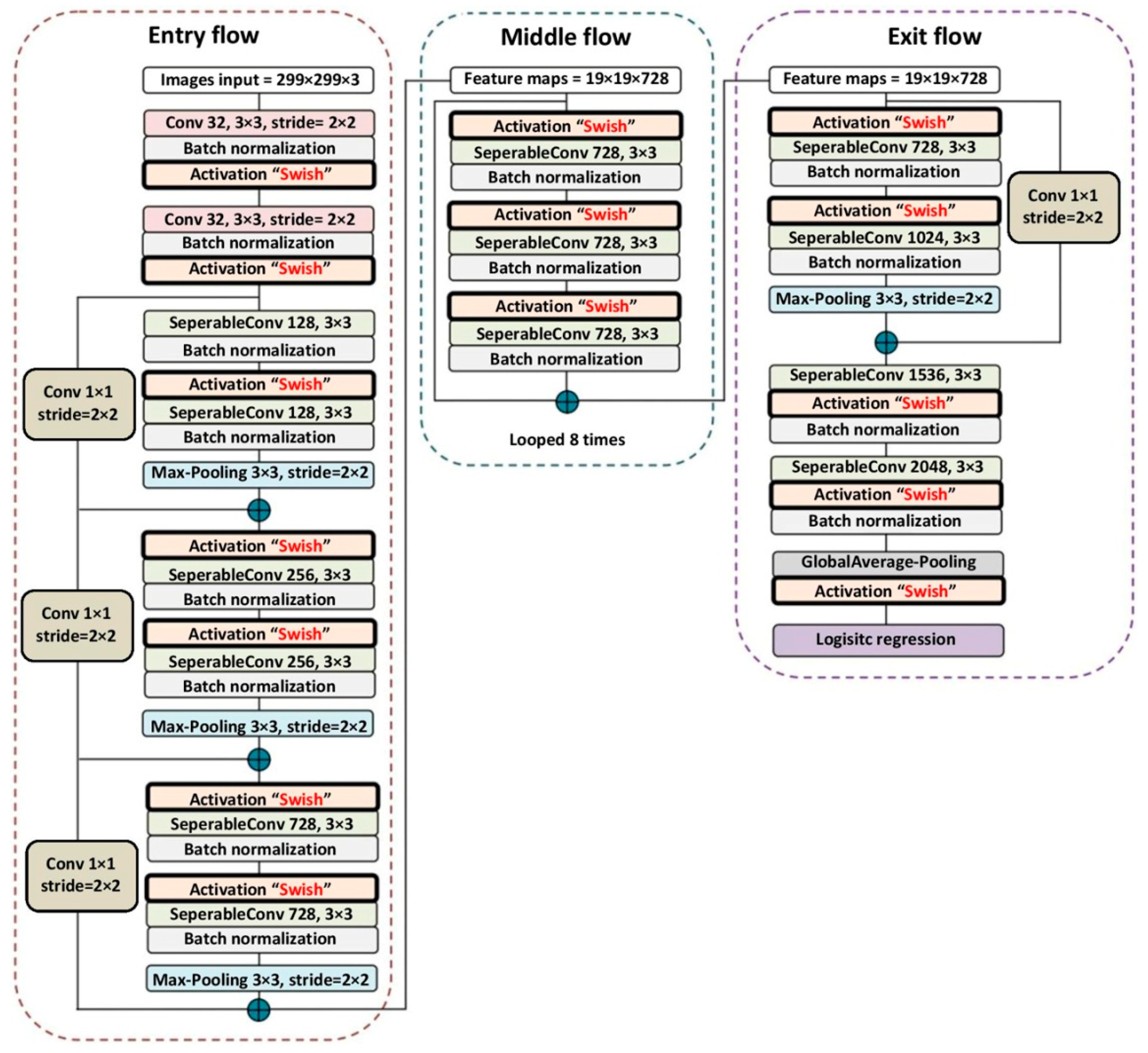
Xception architecture has 36 convolutional layers to generate feature extraction for image classification, which creates 14 modules that punctuate with residual connections excluding the first and last modules. The input image, by requirement size and channels of 299 × 299 × 3, begin the entry flow section in the first module with two convolutional layers by determining the 32 and 64 filters on a kernel size of 3 × 3, and, for the second to fourth modules, employs a kernel size of 3 × 3 and separable convolution filters of 128, 256, and 728, in which the entry flow produces a feature map of 19 × 19 × 728 and goes through loops eight times (fifth to twelfth modules) in the middle flow section by separable convolution filters of 728. After that, the feature map from the middle flow forwards to the final section of the exit flow, in which the thirteenth module employs two size separable convolution filters of 728 and 1024. A final module employs two size separable convolution filters of 1536 and 2048, with added global average-pooling [52] and the fully connected layer before logistic regression as the last layer.

2.2. Swish Activation Function and Modification of Xception with Swish

CNN can improve image classification tasks with appropriate activation functions [47]. Presently, there is widespread use of the activation function known as ReLU, which is also used in the Xception architecture. CNN with ReLU is easy and effective to optimize when the input flow to the ReLU function is positive. However, development of the Swish activation function in recent years has an activation function consequence in cooperated techniques between exhaustive and the searching techniques of reinforcement learning. Swish can improve the CNN of image classification over ReLU [47] in the following function:
S w i s h ( d ) = d S i g m o i d ( β d )
where β represents a per-channel trainable parameter, d indicates the input data, and Sigmoid(βd) is the calculation of the sigmoid function [47], in which the Swish activation function can rewrite the position of the ReLU activation function in the CNN architecture. The proposed image classification model by modification of Xception with Swish is shown in Figure 5.
Figure 5 indicates that in the Xception with Swish architecture, every module stands identically to the original Xception, only ReLU is replaced with Swish in the activation function position. In a minor modification, we add one more Swish after the global average-pooling and before logistic regression. The original Xception model is excellent for image classification. However, improving classification performance is essential for continuous development. We investigated the Swish activation function in order to improve performance. Thus, our new model is based on the original Xception architecture but with applying the Swish activation function to potentially enhance the image classification performance.

3. Materials and Colorectal Polyp Classification Methods

3.1. Colorectal Topogram Image Dataset Preparation and Image Augmentation

The benchmark colonography image datasets in this study were collected from CT_COLONOGRAPHY [53] and the Cancer Genome Atlas of colon adenocarcinoma (TCGA-COAD) [54]. Both datasets were gathered from the public access Cancer Imaging Archive (TCIA) [55], which provides spreadsheet description files of polyps, consistent with prone and supine 3D CT images and 2D topogram images in the Digital Imaging and Communications in Medicine (DICOM) format. Our study focuses on utilizing 2D topogram images, as shown in Figure 6, for training of the image classification model to investigate the potential development of preliminary screening in colorectal diagnosis. For the CT_COLONOGRAPHY dataset, the main dataset, images of 825 colonography patients were collected. However, the dataset actually used a total of 347 patients, divided into three categories. The first category, containing 6 to 9 mm polyps, comprises 69 patients with small size polyps in 125 topogram images. The second category is large, 10 mm polyps, containing 106 topogram images from 35 patients, while the third category consists of 224 topogram images from 243 patient cases of polyp not found. For TCGA-COAD assigned for the extended dataset, 25 patient cases with 30 topogram images were obtained in the second category, large size polyps. In addition, we also classified two classes of polyps for preliminary screening, found from the merging of 106 images of large size and 125 images of small size, resulting in a sum of 231 topogram images in the first category, and using polyp not found for the second category.
However, we considered that our colorectal topogram images were quite small in number and not sufficient for training the image classification model or examining its effect on the overfitting problem. As a solution, several studies suggested the image augmentation method to increase the image dataset and avoid overfitting [1,23,33,43]. We applied the image augmentation method by transformations from 0 to 10 of rotation of left and right, shifting up–right, shifting down–left by 0.5, and cropping the center. After augmentation, the image dataset was increased from 455 images to 2730 images, including the original images. For the two categories, there were 1386 polyp found images and 1344 polyp not found images. For the three categories, there were 798 images of small size polyps, 588 images of large size polyps, and 1344 images of polyp not found, the same as in the two categories.

3.2. Training CNN Image Classification Models

The final colorectal topogram image dataset consisted of 2730 images. We divided the dataset for testing by 10%, or 273 images. The 2457 remaining images were separated into 80% training data, or 1965 images, and 20% validation data, or 492 images. All CNN models in the experiment utilized 50 epochs to perform the training and validation of the dataset, employing a desktop computer comprising an NVIDIA GeForce GTX 1070 graphical processing unit (GPU) with 11 gigabytes of RAM. Training with the GPU is much faster than training without the GPU. The training and validation processes use the deep learning model of transfer learning, which can be run from the Keras [56] library of the GPU version by a backend of the Tensorflow [57] GPU. The implementation was written using Python [58] as the main programming language on a Windows operating system. The specifications of the hardware and software utilized in the experiment are detailed in Table 1. The proposed CNN of Xception with Swish and other CNN models have different requirements for configuration, such as image input size, batch size, optimizer, and learning rate, which reduce the learning rate every three epochs when performance has not improved. CNN model configuration for this work is indicated in Table 2 by the original CNN architecture applying the Swish activation function as an identical configuration.
The configuration in Table 2 was devised based on suggestions from each model’s original paper, since these models can generate excellent performance with the appropriate configuration, depending on the architecture and dataset characterization. However, a significant component of CNN is the optimizers, which need to be defined. Stochastic gradient descent (SGD) [59] and RMSprop [60] are both optimizers that use gradient descent techniques, which are widely used because of their ability to improve CNN performance while generating rapid learning [59,60].

3.3. Comparison of Experimental Results for CNN Image Classification Models

CNN architecture training in this study compared the experimental results between original CNN models and CNN models with the Swish activation function on colorectal polyp classification in the context of preliminary screening. For the two categories of polyp found and polyp not found, classifying was done in three categories, small size, large size, and polyp not found. After finishing training, all CNN model estimations of classification performance in terms of accuracy, precision, recall, and F1 measure can be computed using the following equations:
A c c u r a c y = T P + T N T P + F N + F P + T N
P r e c i s i o n = T P T P + F P
R e c a l l = T P T P + F N
F 1 m e a s u r e = 2 × P r e c i s i o n × R e c a l l P r e c i s i o n + R e c a l l
where TP defines true positive, or the number of input images for each category correctly classified; FP is false positive, indicating the number of incorrectly classified images in the class; TN is true negative, representing number of images correctly classified as not belonging in the class; and FN is false negative, representing images from the class that are incorrectly classified. The experimental results compare two classes without Swish, shown in Table 3, and two classes with Swish, shown in Table 4. Results of three classes were compared: without Swish, as shown in Table 5, and three classes with Swish, shown in Table 6.
A comparison of experimental results was done for the original CNN without Swish to classify two classes, polyp found and polyp not found. Table 3 shows that Xception is the top CNN for the two classifications, producing accuracy of 97.97%, precision of 97.95%, recall of 97.99%, and F1 of 97.97, while spending 62:50 min of training time. Table 4 shows the original CNN with Swish, and the results show that Xception with Swish had improved accuracy of 98.99%, increased precision of 98.99%, recall up to 99.00%, and F1 measure of 98.99% with training time of 67:17 min. The CNN model with the lowest score is VGG16 for both original and with Swish; they produced the same results, with accuracy of 48.17%, precision of 24.09, recall of 50.00%, and F1 measure of 32.51%.
Swish also assisted NASNetMobile and MobileNetV2 with improved performance. NASNetMobile had increased accuracy from 76.71% to 77.64%, precision from 76.71% to 77.69%, recall from 76.64% to 77.72%, and F1 measure from 76.66% to 77.64%. MobileNetV2 had improved accuracy from 69.72% to 71.75%, precision from 69.68% to 71.71%, recall from 69.68% to 71.69%, and F1 measure from 69.68% to 71.70%. In another CNN model, the classification performance was not improved when the Swish activation function was applied. Furthermore, all CNN models had more time consumption than the original.
The comparison of classification performance of the three classes of small size, large size, and polyp not found by the original CNN models is shown in Table 5, which shows that Xception still had the best performance, with accuracy of 90.36%, precision of 88.17%, recall of 88.15%, and F1 measure of 88.12%, with training time of 77:43 min. In Table 6, two classes, including Xception with Swish, had improved classification performance in three classes, achieving accuracy of 91.48%, precision of 91.19%, recall of 90.33%, and F1 measure of 90.73%, with increased training time of 80:34 min. All CNN models also spent more training time for three classes when Swish was applied. For the lowest score, the VGG16 model had accuracy of 48.17%, precision of 16.06%, recall of 33.33%, and F1 measure of 21.67%, meaning the scores are identical for the original and Swish activation function.
For classification into three classes, Swish had improved performance in the CNN models of ResNet50 and NASNetLarge. ResNet50 had increased accuracy from 87.60% to 90.06%, precision from 86.03% to 89.85%, recall from 84.56% to 88.96%, and F1 measure from 85.22% to 89.38%. For NASNetLarge, accuracy increased from 82.12% to 84.05%, precision from 81.13% to 83.43%, recall from 80.22% to 80.60%, and F1 measure from 80.96% to 81.99%.
Considering time consumption for classification performance in the context of the computational complexity of this study, the various models completed the experiment in a short time, but could not generate all evaluation indices (VGG16, InceptionV3, InceptionResNetV2, NASNetMobile, and MobileNetV2) well. After the experiment, some models established good results, but used a lot of time (NASNetLarge). ResNet50 training in a short time produced good results, but not as good as Xception. While the experiment with Xception with Swish required suitable time consumption, it achieved better performance results compared with the other approaches. Therefore, it is observed that Xception with Swish is feasible for preliminary screening of colorectal polyps with high classification performance.

4. Discussion

According to the experimental results, it seems that the original Xception and our proposed model of Xception with Swish can give the probability of classification performance results in both two classes and three classes to develop an image classification system in the context of preliminary colorectal polyp screening. The classification performance of our proposed Xception with Swish model is better than the original Xception model, which is explained in this section, including training and validation history, receiver operating characteristic (ROC) estimation, area under the curve (AUC) generation, confusion matrix, and testing model classification.

4.1. Colorectal Polyp Classification in Two Classes

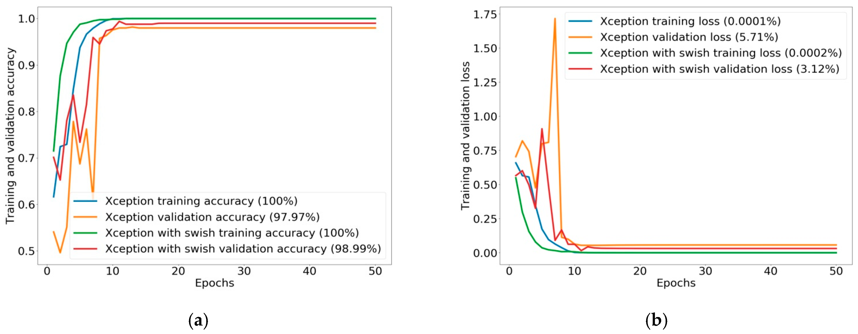
Regarding training and validation history, 50 epochs seemed good enough for our experiment [61,62], as illustrated in Figure 7. Both the original Xception and Xception with Swish raised training accuracy up to 100%, as shown in Figure 7a, and decreased training and validation loss very low, down to 0.0001% and 0.0002%, respectively, as shown in Figure 7b. However, Xception with Swish generated validation accuracy of 98.99% with validation loss of 3.12%, which is better than the accuracy of 97.97% with validation loss of 5.71% for Xception. When considering the validation history, we found that the validation accuracy of Xception with Swish had higher scores and was approximately stable above the Xception validation history at nine epochs until the final epochs. In other words, validation loss of Xception with Swish started lower than Xception at the same nine epochs to the final epochs.
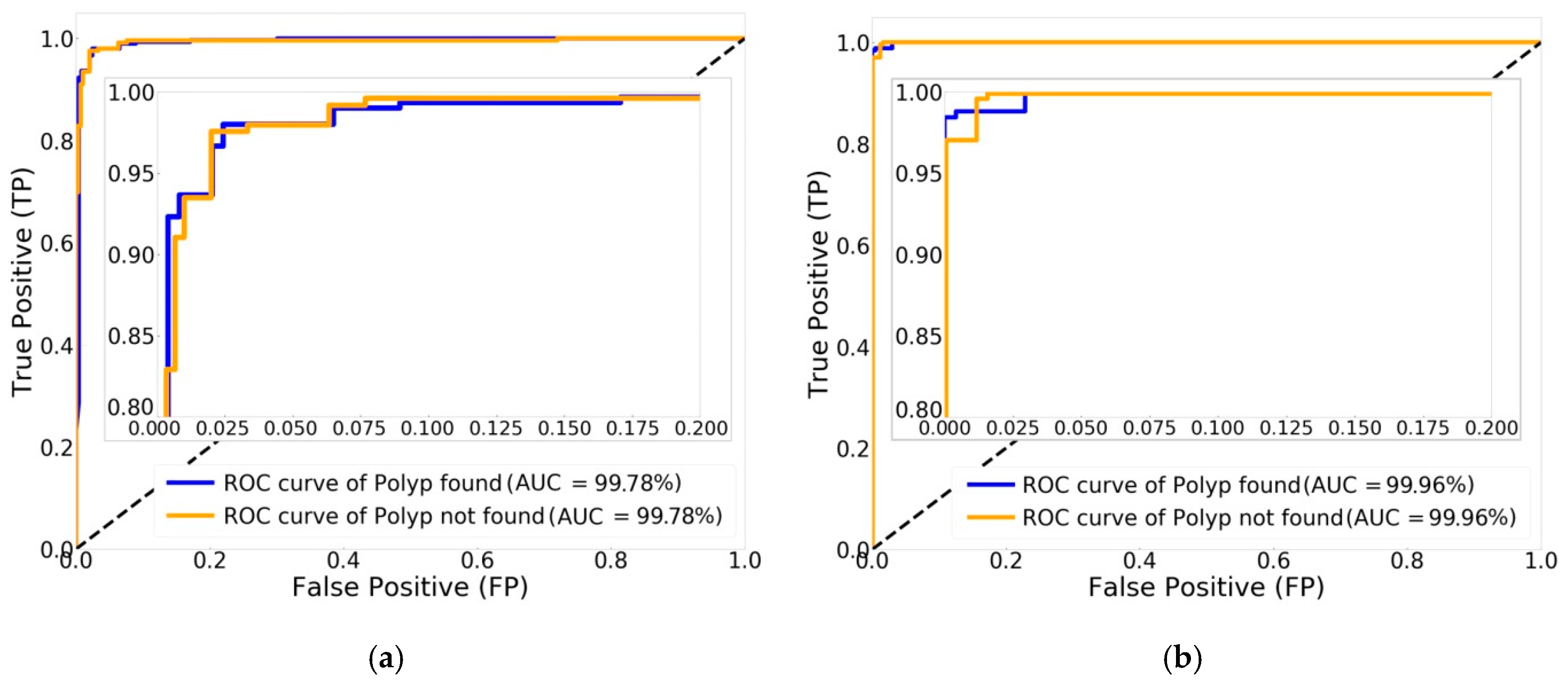
A comparison of ROC curves and AUC generated by TP and FP rates in the classification performance of two classes is illustrated in Figure 8a for Xception, and in Figure 8b for Xception with Swish. Although the curves of Xception for both classes are close to 100%, creating an AUC of 99.78%, Xception with Swish generated more, with an AUC of 99.96% in both classes, polyp found and polyp not found.
In describing the model classification performance on the validation data, which was determined as 20%, or 492 images, for classifying into two classes, a confusion matrix of true class and predicted class for Xception was drawn, as shown in Figure 9a; the confusion matrix of Xception with Swish is shown in Figure 9b. The validation set of 492 images was split into two, 255 images of polyp found, and 237 images of polyp not found. Xception correctly classified polyps found in 248 images, with mistakes in seven images, and polyp not found in 234 images, with three images misclassified. Comparing the confusion matrices, our proposed Xception with Swish model generated better classification of polyps found in 251 images, with four images misclassified, and polyp not found in 236 images, with one image incorrectly classified.
The trained and validated Xception and Xception with Swish models for colorectal polyp classification in two classes were ready to compare the testing for classification of 273 external images (10% of all images), excluding training and validation processes. The comparison results are shown in Table 7.
Table 7 presents a total of 273 testing images, divided into 138 images of polyp found and 135 images of polyp not found. The original Xception model generated true predictions of polyps in 136 images, or 98.55%, and polyp not found in 133 images, or 98.51%, and false predictions of polyp found in two images, or 1.45%, and polyp not found in two images, or 1.48%. Xception with Swish produced true predictions of polyp found in 138 images, or 100%, and polyp not found in 134 images, or 99.25%, with false prediction of one image, or 0.74%.
According to the total true predictions of 269 images by Xception, at 98.51%, with total false predictions of four images, or 1.47%, compared to the true predictions of Xception with Swish, 272 images, at 99.63%, and false prediction of only one image, or 0.37%, the results from testing data show that Xception with Swish improved classification compared to Xception alone by three images, accounting for 1.12%.

4.2. Colorectal Polyp Size Classification for Three Classes

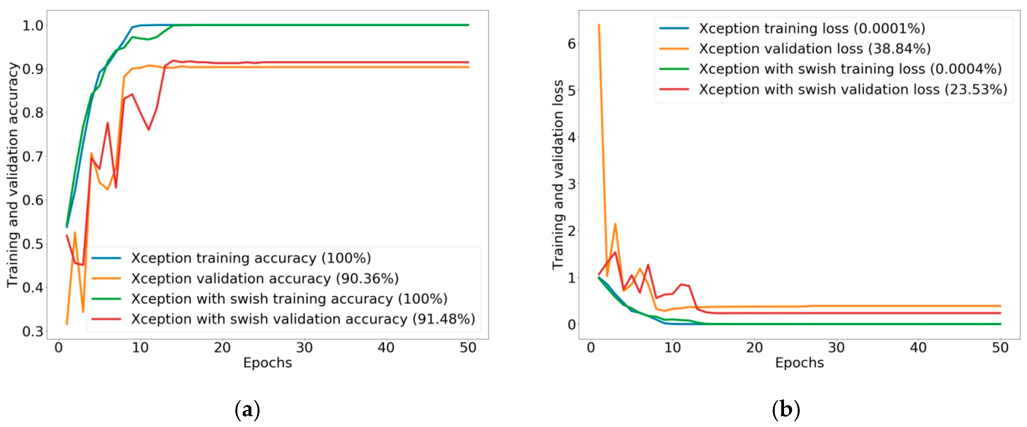
The historical training and validation of accuracy in Figure 10a and loss in Figure 10b for classifying three classes show that Xception and Xception with Swish are still outstanding, with high training accuracy of 100% and the lowest loss rates of 0.0001% and 0.0004%, respectively. Nevertheless, when determining validation accuracy and loss of Xception with Swish, it still gives high accuracy of 91.48% with low loss of 23.53%, while Xception generates accuracy of 90.36% with validation loss of 38.84%. By adding a class to the validation accuracy and loss, classification performance will drop compared to two classes.
Similar to the results of classification performance, the ROC curve and AUC, illustrated in Figure 11a for Xception, for the three classes show an AUC of 98.04% for small size polyps, 97.47% for large size polyps, and 99.80% for polyp not found. The Xception with Swish model had better classification performance, shown in Figure 11b: AUC of 98.22% for small size polyps, 97.85% for large size polyps, and 99.89% for polyp not found.
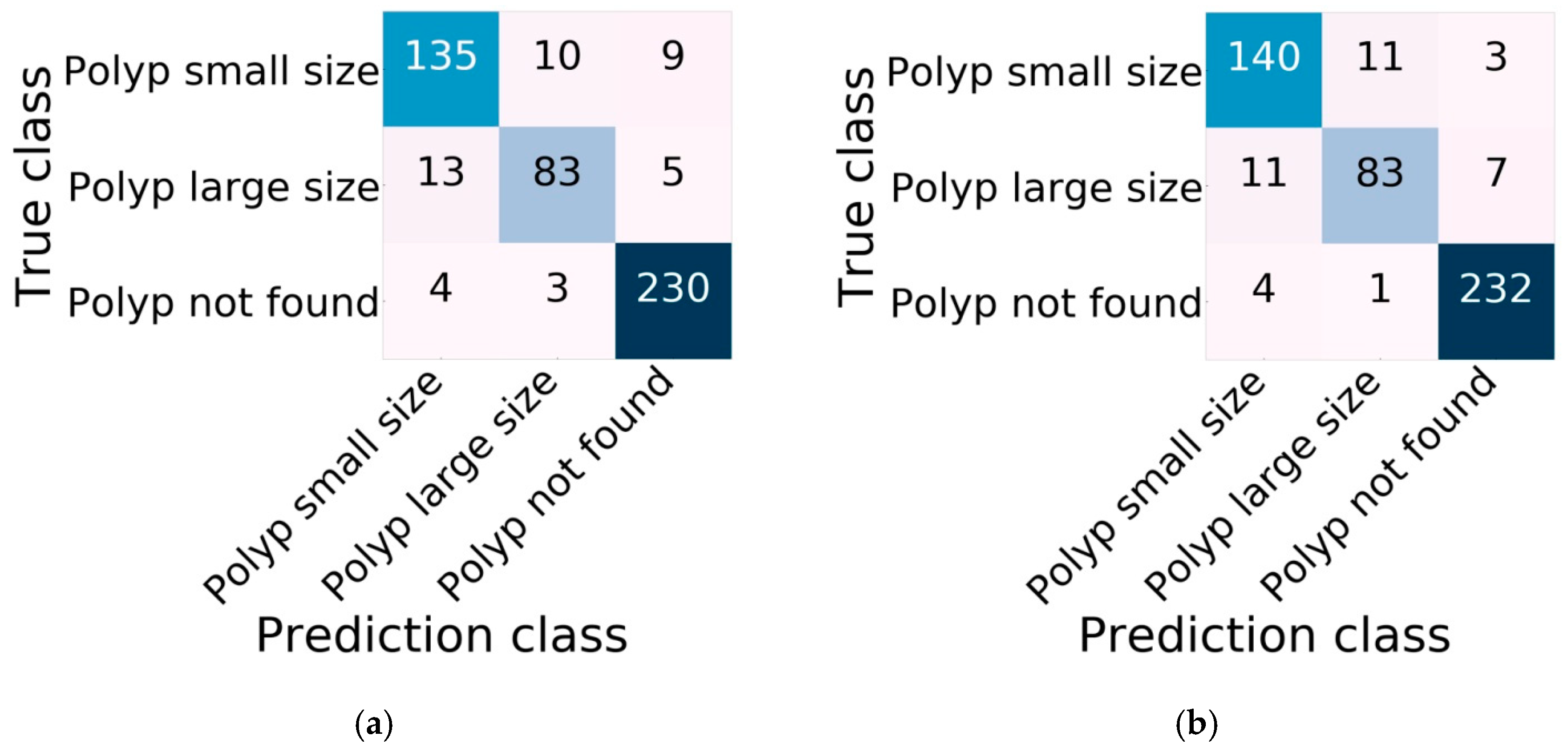
The confusion matrix of classification performance on validation data with three classes for Xception is shown in Figure 12a, and the confusion matrix of Xception with Swish is shown in Figure 12b. The validation images were divided for the three classes as follows: small size polyps in 154 images, large size polyps in 101 images, and polyp not found in 237 images. Xception correctly classified small size polyps in 135 images and incorrectly in 19 images, correctly classified large size polyps in 83 images and incorrectly in 18 images, and correctly classified polyp not found in 230 images and incorrectly in seven images. The proposed model of Xception with Swish had better classification than Xception in the three classes: in the first class, it correctly classified 140 images and incorrectly classified 14 images, in the second class it correctly classified 83 images and incorrectly classified 18 images, and in the third class it correctly classified 232 images and incorrectly classified five images. The testing for classification of both models employed another 273 images for the three classes. The results are illustrated in Table 8.
The comparison of results of testing for classification in Table 8 shows that the testing data were separated into three classes: 79 images for small size polyps, 59 images for large size polyps, and 135 images for polyp not found. The original Xception achieved true prediction of small size polyps in 48 images, accounting for 60.75%, with false prediction of 31 images, or 39.24%; true prediction of large size polyps in 37 images, or 62.71%, with false prediction of 22 images, or 37.28%; and true prediction of polyp not found in 134 images, or 99.25%, and false prediction of one image, or 0.74%. The proposed Xception with Swish had true prediction of small size polyps in 49 images, or 62.02%, and large size polyps in 37 images, or 62.71%. In the class of polyp not found, it obtained 135 images, or 100%, without false any predictions.
In the experimental results of testing for classification in three classes, we observed that Xception with Swish classified better than the original Xception. The total true prediction of Xception obtained 219 images, accounting for 80.21%, and total false prediction was 54 images, accounting for 19.78%, compared to total true prediction by Xception with Swish of 221 images, or 80.95%, with total false prediction of 52 images, or 19.04%. Thus, Xception with the Swish activation function enhanced the classification performance for the three classes by more two images, or 0.38%, compared to Xception alone.
The results of this work may be further improved in future work, which may focus on reducing the false negative (FN) results. Patients in some cases have colorectal polyps that the model does not identify or predicts incorrectly. Also, the model in this study produced false predictions for both two and three classes, which may result in false predictions that also include false negatives. In this case, we investigated some FN reduction techniques that could be adopted with our proposed method in future studies, such as combining with other kinds of medical images [63] such as CT, MRI, and ultrasound. Another method applies the texture descriptor technique to identify local image patterns [64] and train the model, which may reduce the number of FN results.

5. Conclusions

CRC is a form of cancer that is a leading cause of human mortality and is increasing among younger generations. Thus, people without data should undergo CRC screening. A 2D topogram image can be generated for screening and planning before advancing to the next procedure. The deep learning technique of CNN is being used to generate effective models of image classification, especially in medical tasks for colorectal polyp diagnosis. However, it has not yet been utilized in the CNN method with colorectal topogram images, which could be used to assist physicians in preliminary screening and rapid diagnosis.
The use of an activation function, Swish, can improve the classification accuracy of CNN. There has never been a study about applying Swish with CNN of Xception architecture. Replacing the ReLU inside Xception with Swish may enhance the performance of image classification when compared to the original Xception and other CNN architectures. The purpose of the paper was to apply a new modification of Xception with the Swish activation function and discover the possibility of developing a novel preliminary screening system for colorectal polyps in the training of our proposed model with benchmark colonography of topogram image datasets and using an image augmentation method to enhance the image dataset. The proposed method was used in the context of colorectal screening to classify two classes of polyps, found and not found, and three size classifications of small, large, and polyp not found. Furthermore, the experimental results were compared with the original Xception and other CNN architectures using the modified architecture with Swish.
In the comparison of experimental results of classifying the two classes of polyp found and polyp not found, Xception was the best in the original CNN group, with an evaluation performance of 97.97%. However, the results show that Xception with Swish was improved, achieving increased classification performance of 98.99%, using more training time with the Swish activation function. The experimental results in the classification performance of two classes were also explained by ROC curve and AUC. Xception with Swish created ROC curves of nearly 100% with AUC of 99.96%, which is greater than the original Xception, with an AUC of 99.78%. With validation image data of 492 images split into two classes of polyps, 255 images were found, while 237 images were not found. The classification performance for validation demonstrated that Xception with Swish generated better classification than the original Xception in the class of polyp found, with 251 images correctly classified and four images misclassified, and in the class of polyp not found, with 236 images correctly classified and one image misclassified. Summarizing the validation image data for Xception with Swish, 487 images were correctly classified from a total of 492 images, while there were only five incorrectly classified images. For testing classification of two classes by applying 273 external images at 100%, the testing data show that Xception with Swish had true predictions for a total of 272 images, accounting for 99.63%, with false prediction of one image, or 0.37%, compared to true prediction by Xception of 269 images, or 98.51%, with false prediction of four images, or 1.47%.
The three classes were defined as small size polyps, large size polyps, and polyp not found. In a comparison of evaluation classification performance, the Xception with Swish model was still improved, but more training time was needed for classification of added classes, increasing the accuracy to 91.48%. Another evaluation score also increased to 90%, while the original Xception produced accuracy of 90.36% by other evaluation indices based on 88%. For the ROC curve and AUC of classification in three classes, Xception showed an AUC of 98.04% for small size polyps, 97.47% for large size polyps, and 99.80% for polyp not found. Xception with Swish showed improved classification performance, with an AUC of 98.22% for small size polyps, 97.85% for large size polyps, and 99.89% for polyp not found.
The confusion matrix of classification performance on validation data was divided into three classes, with 154 images of small size polyps, 101 images of large size polyps, and 237 images of polyp not found. The proposed Xception with Swish model correctly classified small size polyps in 140 images, with misclassification of 14 images; correctly classified large size polyps in 83 images, with 18 images misclassified; and correctly classified 232 images of polyp not found, with five images misclassified. Xception with Swish correctly classified a total of 455 images, and incorrectly classified a total of 37 images. In comparison, the original Xception correctly classified a total of 448 images, with 44 images incorrectly classified. The totals of correctly and incorrectly classified images of the three classes indicate that Xception with Swish achieved better image classification than the original Xception, with many correctly classified and few incorrectly classified images. For testing classification of three classes, Xception with Swish still showed better classification, with total true predictions of 221 images, or 80.95%, and false predictions of 52 images, or 19.04%, compared to Xception, with total true predictions of 219 images, or 80.21%, and false predictions of 54 images, or 19.78%.
According to all of the experimental results in this study, the proposed Xception with Swish model achieved better image classification performance than several original CNN techniques, providing a reasonable basis and possibility for further development of a novel preliminary screening system for colorectal polyps to assist physicians in preliminary screening and rapid diagnosis.

Author Contributions

Conceptualization, N.J. and C.-F.T.; Data curation, C.-E.T. and P.W.; Formal analysis, N.J.; Funding acquisition, C.-F.T.; Investigation, N.J. and C.-F.T.; Methodology, N.J. and C.-F.T.; Project administration, C.-F.T.; Resources, N.J.; Software, N.J.; Supervision, C.-F.T.; Validation, C.-E.T. and P.W.; Visualization, N.J.; Writing—original draft, N.J.; Writing—review & editing, N.J. and C.-F.T.

Funding

This research was funded by the Ministry of Science and Technology, Republic of China, Taiwan, grant numbers MOST-107-2637-E-020-006, MOST-108-2637-E-020-003, MOST-108-2321-B-020-003, and MOST-107-2321-B-020-005.

Acknowledgments

The authors would like to express their sincere gratitude to the anonymous reviewers for their useful comments and suggestions for improving the quality of this paper, and we thank the Department of Tropical Agriculture and International Cooperation, Department of Management Information Systems, National Pingtung University of Science and Technology, and Taiwan and Ministry of Science and Technology, Republic of China, Taiwan, for supporting this research.

Conflicts of Interest

The authors declare no conflict of interest.

References

  1. Hu, Z.; Tang, J.; Wang, Z.; Zhang, K.; Zhang, L.; Sun, Q. Deep learning for image-based cancer detection and diagnosis − A survey. Pattern Recogn. 2018, 83, 134–149. [Google Scholar] [CrossRef]
  2. Ponzio, F.; Macii, E.; Ficarra, E.; Cataldo, S. Colorectal Cancer Classification using Deep Convolutional Networks-An Experimental Study. In Proceedings of the 11th International Joint Conference on Biomedical Engineering Systems and Technologies (BIOSTEC 2018), Funchal, Madeira, Portugal, 19–21 January 2018; pp. 58–66. [Google Scholar]
  3. Kasi, P.M.; Shahjehan, F.; Cochuyt, J.; Li, Z.; Colibaseanu, D.T.; Merchea, A. Rising Proportion of Young Individuals With Rectal and Colon Cancer. Clin. Colorectal. Canc. 2019, 18, e87–e95. [Google Scholar] [CrossRef] [PubMed] [Green Version]
  4. American Cancer Society. Colorectal Cancer Facts & Figures 2017–2019. 2017. Available online: https://www.cancer.org/content/dam/cancer-org/research/cancer-facts-and-statistics/colorectal-cancer-facts-and-figures/colorectal-cancer-facts-and-figures-2017-2019.pdf (accessed on 9 September 2019).
  5. Senore, C.; Bellisario, C.; Segnan, N. Distribution of colorectal polyps: Implications for screening. Best Pract. Res. Clin. Gastroenterol. 2017, 31, 481–488. [Google Scholar] [CrossRef] [PubMed]
  6. Van Lanschot, M.C.J.; Carvalho, B.; Rausch, C.; Snaebjornsson, P.; van Engeland, M.; Kuipers, E.J.; Stoker, J.; Tutein Nolthenius, C.J.; Dekker, E.; Meijer, G.A. Molecular profiling of longitudinally observed small colorectal polyps: A cohort study. EBioMedicine 2019, 39, 292–300. [Google Scholar] [CrossRef] [Green Version]
  7. Balashova, E.; Wang, J.; Singh, V.; Georgescu, B.; Teixeira, B.; Kapoor, A. 3D Organ Shape Reconstruction from Topogram Images. arXiv 2019, arXiv:1904.00073. [Google Scholar]
  8. Mayo-Smith, W.W.; Hara, A.K.; Mahesh, M.; Sahani, D.V.; Pavlicek, W. How I Do It: Managing Radiation Dose in CT. Radiology 2014, 273, 657–672. [Google Scholar] [CrossRef] [Green Version]
  9. Godkhindi, A.M.; Gowda, R.M. Automated detection of polyps in CT colonography images using deep learning algorithms in colon cancer diagnosis. In Proceedings of the 2017 International Conference on Energy, Communication, Data Analytics and Soft Computing (ICECDS), Chennai, Tamil Nadu, India, 1–2 August 2017; pp. 1722–1728. [Google Scholar]
  10. Pang, S.; Yu, Z.; Orgun Mehmet, A. A novel end-to-end classifier using domain transferred deep convolutional neural networks for biomedical images. Comput. Methods Programs Biomed. 2017, 140, 283–293. [Google Scholar] [CrossRef]
  11. Amato, F.; Castiglione, A.; Mercorio, F.; Mezzanzanica, M.; Moscato, V.; Picariello, A.; Sperlì, G. Multimedia story creation on social networks. Future Gener. Comput. Syst. 2018, 86, 412–420. [Google Scholar] [CrossRef]
  12. Amato, F.; Castiglione, A.; Moscato, V.; Picariello, A.; Sperlì, G. Multimedia summarization using social media content. Multimed. Tools Appl. 2018, 77, 17803–17827. [Google Scholar] [CrossRef]
  13. Shin, Y.; Balasingham, I. Automatic polyp frame screening using patch based combined feature and dictionary learning. Comput. Med. Imag. Grap. 2018, 69, 33–42. [Google Scholar] [CrossRef]
  14. Lecun, Y.; Bottou, L.; Bengio, Y.; Haffner, P. Gradient-based learning applied to document recognition. Proc. IEEE 1998, 86, 2278–2324. [Google Scholar] [CrossRef] [Green Version]
  15. Hinton, G.E.; Osindero, S.; Teh, Y.W. A fast learning algorithm for deep belief nets. Neural. Comput. 2006, 18, 1527–1554. [Google Scholar] [CrossRef] [PubMed]
  16. Hinton, G.E.; Salakhutdinov, R.R. Reducing the dimensionality of data with neural networks. Science 2006, 313, 504–507. [Google Scholar] [CrossRef] [PubMed] [Green Version]
  17. Deng, J.; Dong, W.; Socher, R.; Li, L.; Li, K.; Li, F.F. ImageNet: A Large-Scale Hierarchical Image Database. In Proceedings of the IEEE Conference on Computer Vision and Pattern Recognition (CVPR’09), MiamiBeach, FL, USA, 20–25 June 2009. [Google Scholar]
  18. Gong, K.; Guan, J.; Kim, K.; Zhang, X.; Yang, J.; Seo, Y.; El Fakhri, G.; Qi, J.; Li, Q. Iterative PET Image Reconstruction Using Convolutional Neural Network Representation. IEEE T. Med. Imaging 2019, 38, 675–685. [Google Scholar] [CrossRef] [PubMed]
  19. Banerjee, I.; Ling, Y.; Chen, M.; Hasan, S.; Langlotz, C.; Moradzadeh, N.; Chapman, B.; Amrhein, T.; Mong, D.; Rubin, D.; et al. Comparative effectiveness of convolutional neural network (CNN) and recurrent neural network (RNN) architectures for radiology text report classification. Artif. Intell. Med. 2019, 97, 79–88. [Google Scholar] [CrossRef] [PubMed]
  20. Huang, Y.; Xu, J.; Zhou, Y.; Tong, T.; Zhuang, X. The Alzheimer’s Disease Neuroimaging Initiative. Diagnosis of Alzheimer’s Disease via Multi-Modality 3D Convolutional Neural Network. arXiv 2019, arXiv:1902.09904. [Google Scholar]
  21. Zhang, H.; Wang, A.; Li, D.; Xu, W. DeepVoice: A voiceprint-based mobile health framework for Parkinson’s disease identification. In Proceedings of the 2018 IEEE EMBS International Conference on Biomedical & Health Informatics (BHI), Las Vegas, NV, USA, 4–7 March 2018; pp. 214–217. [Google Scholar]
  22. Özyurt, F.; Sert, E.; Avci, E.; Dogantekin, E. Brain tumor detection based on Convolutional Neural Network with neutrosophic expert maximum fuzzy sure entropy. Measurement 2019, 147, 106830. [Google Scholar] [CrossRef]
  23. Wang, C.; Elazab, A.; Jia, F.; Wu, J.; Hu, Q. Automated chest screening based on a hybrid model of transfer learning and convolutional sparse denoising autoencoder. BioMed. Eng. OnLine 2018, 17, 63. [Google Scholar] [CrossRef]
  24. Alom, M.Z.; Yakopcic, C.; Nasrin, M.S.; Taha, T.M.; Asari, V.K. Breast Cancer Classification from Histopathological Images with Inception Recurrent Residual Convolutional Neural Network. J. Digit. Imaging 2019, 32, 605–617. [Google Scholar] [CrossRef] [Green Version]
  25. Maier, A.; Syben, C.; Lasser, T.; Riess, C. A gentle introduction to deep learning in medical image processing. Z. Med. Phys. 2019, 29, 86–101. [Google Scholar] [CrossRef]
  26. Urban, G.; Tripathi, P.; Alkayali, T.; Mittal, M.; Jalali, F.; Karnes, W.; Baldi, P. Deep Learning Localizes and Identifies Polyps in Real Time With 96% Accuracy in Screening Colonoscopy. Gastroenterology 2019, 155, 1069–1078, e1068. [Google Scholar] [CrossRef] [PubMed]
  27. Diamantis, D.E.; Iakovidis, D.K.; Koulaouzidis, A. Look-behind fully convolutional neural network for computer-aided endoscopy. Biomed. Signal Proces. 2019, 49, 192–201. [Google Scholar] [CrossRef]
  28. Soomro, M.H.; De Cola, G.; Conforto, S.; Schmid, M.; Giunta, G.; Guidi, E.; Neri, E.; Caruso, D.; Ciolina, M.; Laghi, A. Automatic segmentation of colorectal cancer in 3D MRI by combining deep learning and 3D level-set algorithm-a preliminary study. In Proceedings of the 2018 IEEE 4th Middle East Conference on Biomedical Engineering (MECBME), Tunis, Tunisia, 28–30 March 2018; pp. 198–203. [Google Scholar]
  29. Huang, Y.; Dou, Q.; Wang, Z.; Liu, L.; Wang, L.; Chen, H.; Heng, P.; Xu, R. HL-FCN: Hybrid loss guided FCN for colorectal cancer segmentation. In Proceedings of the 2018 IEEE 15th International Symposium on Biomedical Imaging (ISBI 2018), Washington, DC, USA, 4–7 April 2018; pp. 195–198. [Google Scholar]
  30. Rie, T.; Janne, J.; Näppi, J.O.; Nadja, K.; Toru, H.; Se, H.K.; Daniele, R.; Hiroyuki, Y. Deep Learning Electronic Cleansing for Single-and Dual-Energy CT Colonography. Radiographics 2018, 38, 2034–2050. [Google Scholar]
  31. Zhang, S.; Han, F.; Liang, Z.; Tan, J.; Cao, W.; Gao, Y.; Pomeroy, M.; Ng, K.; Hou, W. An investigation of CNN models for differentiating malignant from benign lesions using small pathologically proven datasets. Comput. Med. Imag. Grap. 2019, 77, 101645. [Google Scholar] [CrossRef]
  32. Wang, P.; Xiao, X.; Glissen Brown, J.R.; Berzin, T.M.; Tu, M.; Xiong, F.; Hu, X.; Liu, P.; Song, Y.; Zhang, D.; et al. Development and validation of a deep-learning algorithm for the detection of polyps during colonoscopy. Nat. Biomed. Eng. 2018, 2, 741–748. [Google Scholar] [CrossRef] [PubMed]
  33. Zhang, R.; Zheng, Y.; Poon, C.C.Y.; Shen, D.; Lau, J.Y.W. Polyp detection during colonoscopy using a regression-based convolutional neural network with a tracker. Pattern Recogn. 2018, 83, 209–219. [Google Scholar] [CrossRef] [PubMed]
  34. Akbari, M.; Mohrekesh, M.; Nasr-Esfahani, E.; Soroushmehr, S.M.; Karimi, N.; Samavi, S.; Najarian, K. Polyp Segmentation in Colonoscopy Images Using Fully Convolutional Network. In Proceedings of the 2018 40th Annual International Conference of the IEEE Engineering in Medicine and Biology Society (EMBC), Honolulu, HI, USA, 18–21 July 2018; pp. 69–72. [Google Scholar]
  35. Byrne, M.F.; Chapados, N.; Soudan, F.; Oertel, C.; Linares Pérez, M.; Kelly, R.; Iqbal, N.; Chandelier, F.; Rex, D.K. Real-time differentiation of adenomatous and hyperplastic diminutive colorectal polyps during analysis of unaltered videos of standard colonoscopy using a deep learning model. Gut 2019, 68, 94–100. [Google Scholar] [CrossRef] [Green Version]
  36. Sornapudi, S.; Meng, F.; Yi, S. Region-Based Automated Localization of Colonoscopy and Wireless Capsule Endoscopy Polyps. Appl. Sci. 2019, 9, 2404. [Google Scholar] [CrossRef] [Green Version]
  37. Muhammad, S.; Ruqayya, A.; Muhammad, M.F.; Ayesha, A.; David, S.; Nasir, M.R. Context-Aware Convolutional Neural Network for Grading of Colorectal Cancer Histology Images. arXiv 2019, arXiv:1907.09478. [Google Scholar]
  38. Kather, J.N.; Krisam, J.; Charoentong, P.; Luedde, T.; Herpel, E.; Weis, C.; Gaiser, T.; Marx, A.; Valous, N.A.; Ferber, D.; et al. Predicting survival from colorectal cancer histology slides using deep learning: A retrospective multicenter study. PLOS Med. 2019, 16, e1002730. [Google Scholar] [CrossRef]
  39. Krizhevsky, A.; Sutskever, I.; Hinton, G.E. Imagenet classification with deep convolutional neural networks. In Advances in Neural Information Processing Systems; Curran Associates, Inc.: New York, NY, USA, 2012; pp. 1097–1105. [Google Scholar]
  40. Simonyan, K.; Zisserman, A. Very deep convolutional networks for large-scale image recognition. arXiv 2014, arXiv:1409.1556. [Google Scholar]
  41. Szegedy, C.; Liu, W.; Jia, Y.; Sermanet, P.; Reed, S.; Anguelov, D.; Erhan, D.; Erhan, V.; Rabinovich, A. Going deeper with convolutions. In Proceedings of the 2015 IEEE Conference on Computer Vision and Pattern Recognition (CVPR), Boston, MA, USA, 7–12 June 2015; pp. 1–9. [Google Scholar]
  42. He, K.; Zhang, X.; Ren, S.; Sun, J. Deep residual learning for image recognition. In Proceedings of the 2016 IEEE Conference on Computer Vision and Pattern Recognition (CVPR), Las Vegas, NV, USA, 27–30 June 2016; pp. 770–778. [Google Scholar]
  43. Gu, J.; Wang, Z.; Kuen, J.; Ma, L.; Shahroudy, A.; Shuai, B.; Liu, T.; Wang, X.; Wang, G.; Cai, J.; et al. Recent advances in convolutional neural networks. Pattern Recogn. 2018, 77, 354–377. [Google Scholar] [CrossRef] [Green Version]
  44. Chollet, F. Xception: Deep learning with depthwise separable convolutions. arXiv 2016, arXiv:1610.02357. [Google Scholar]
  45. Szegedy, C.; Vanhoucke, V.; Ioffe, S.; Shlens, J.; Wojna, Z. Rethinking the inception architecture for computer vision. arXiv 2015, arXiv:1512.00567. [Google Scholar]
  46. Vinod, N.; Geoffrey, E.H. Rectified linear units improve restricted boltzmann machines. In Proceedings of the 27th International Conference on Machine Learning (ICML), Haifa, Israel, 21–24 June 2010; pp. 807–814. [Google Scholar]
  47. Ramachandran, P.; Zoph, B.; Le, Q.V. Searching for activation functions. In Proceedings of the International Conference on Learning Representations, Vancouver, BC, Canada, 30 April–3 May 2018. [Google Scholar]
  48. Zoph, B.; Vasudevan, V.; Shlens, J.; Le, Q.V. Learning transferable architectures for scalable image recognition. arXiv 2017, arXiv:1707.07012. [Google Scholar]
  49. Szegedy, C.; Ioffe, S.; Vanhoucke, V.; A Alemi, A. Inception-v4, inception-resnet and the impact of residual connections on learning. In Proceedings of the Thirty-First AAAI Conference on Artificial Intelligence, San Francisco, CA, USA, 4–9 February 2017; pp. 4278–4284. [Google Scholar]
  50. Ioffe, S.; Szegedy, C. Batch normalization: Accelerating deep network training by reducing internal covariate shift. In Proceedings of the 32th International Conference on Machine Learning (ICML), Lille, France, 6–11 July 2015; pp. 448–456. [Google Scholar]
  51. Howard, A.G.; Zhu, M.; Chen, B.; Kalenichenko, D.; Wang, W.; Weyand, T.; Andreetto, M.; Adam, H. MobileNets: Efficient Convolutional Neural Networks for Mobile Vision Applications. arXiv 2017, arXiv:1704.04861. [Google Scholar]
  52. Zhou, B.; Khosla, A.; Lapedriza, A.; Oliva, A.; Torralba, A. Learning Deep Features for Discriminative Localization. In Proceedings of the 2016 IEEE Conference on Computer Vision and Pattern Recognition (CVPR), Las Vegas, NV, USA, 27–30 June 2016; pp. 2921–2929. [Google Scholar]
  53. Smith, K.; Clark, K.; Bennett, W.; Nolan, T.; Kirby, J.; Wolfsberger, M.; Moulton, J.; Vendt, B.; Freymann, J. Data From CT_COLONOGRAPHY. The Cancer Imaging Archive. 2015. Available online: http://doi.org/10.7937/K9/TCIA.2015.NWTESAY1 (accessed on 9 September 2019).
  54. Kirk, S.; Lee, Y.; Sadow, C.A.; Levine, S.; Roche, C.; Bonaccio, E.; Filiippini, J. Radiology Data from The Cancer Genome Atlas Colon Adenocarcinoma [TCGA-COAD] collection. The Cancer Imaging Archive. 2016. Available online: http://doi.org/10.7937/K9/TCIA.2016.HJJHBOXZ (accessed on 9 September 2019).
  55. Clark, K.; Vendt, B.; Smith, K.; Freymann, J.; Kirby, J.; Koppel, P.; Moore, S.; Phillips, S.; Maffitt, D.; Pringle, M.; et al. The Cancer Imaging Archive (TCIA): Maintaining and Operating a Public Information Repository. J. Digit. Imaging 2013, 26, 1045–1057. [Google Scholar] [CrossRef] [Green Version]
  56. Chollet, F. Keras. 2015. Available online: https://github.com/fchollet/keras (accessed on 5 September 2019).
  57. Abadi, M.; Agarwal, A.; Barham, P.; Brevdo, E.; Chen, Z.; Citro, C.; Corrado, G.S.; Davis, A.; Dean, J.; Devin, M.; et al. Tensor-Flow: Large-scale machine learning on heterogeneous systems. arXiv 2015, arXiv:1603.04467. [Google Scholar]
  58. Van Rossum, G. Python Tutorial; Technical Report CS-R9526; Centrum voor Wiskunde en Informatica (CWI): Amsterdam, The Netherlands, May 1995; Python Software Foundation; Available online: https://www.python.org/ (accessed on 5 September 2019).
  59. Ruder, S. An overview of gradient descent optimization algorithms. arXiv 2016, arXiv:1609.04747. [Google Scholar]
  60. Hinton, G.E. Tutorial on deep learning in: IPAM Graduate Summer School: Deep Learning, Feature Learning, Los Angeles, CA, USA, 9–27 July 2012. 262. Available online: http://www.ipam.ucla.edu/programs/summer-schools/graduate-summer-school-deep-learning-feature-learning/(accessed on 9 September 2019).
  61. Hassan, S.-U.; Imran, M.; Iqbal, S.; Aljohani, N.R.; Nawaz, R. Deep context of citations using machine-learning models in scholarly full-text articles. Scientometrics 2018, 117, 1645–1662. [Google Scholar] [CrossRef]
  62. Wang, J. A deep learning approach for atrial fibrillation signals classification based on convolutional and modified Elman neural network. Future Gener. Comput. Syst. 2020, 102, 670–679. [Google Scholar] [CrossRef]
  63. Hyun, S.J.; Kim, E.K.; Yoon, J.H.; Moon, H.J.; Kim, M.J. Adding MRI to ultrasound and ultrasound-guided fine-needle aspiration reduces the false-negative rate of axillary lymph node metastasis diagnosis in breast cancer patients. Clin. Radiol. 2015, 70, 716–722. [Google Scholar] [CrossRef] [PubMed]
  64. Nosheen, F.; Khan, S.; Iqbal, K.; Sharif, M.; Hussain, M.; Naz, R. False positive and false negative reduction in digital mammograms using binary rotation invariant and noise tolerant texture descriptor. In Proceedings of the 2017 International Conference on Communication Technologies (ComTech), Islamabad, Pakistan, 19–21 April 2017; pp. 186–190. [Google Scholar]
Figure 1. Preliminary colorectal polyp screening system for colonoscopy diagnosis.
Mathematics 07 01170 g001
Figure 2. Comparison of Inception module [41] and Xception module [44]: (a) module of Inception v3 [45] on separate 1 × 1 convolution and average pooling; (b) Xception module uses one 1 × 1 convolution to output channels and separates to 3 × 3 convolutions without average pooling.
Mathematics 07 01170 g002
Figure 3. Each color channel 3 × 3 filter is split in the depth-wise convolution linked to 1 × 1 point-wise convolution, which uses 1 × 1 filter size to produce a linear combination.
Mathematics 07 01170 g003
Figure 4. Residual connection diagram procedure showing (a) the original idea of ResNet architecture using residual connections; (b) the adoption of residual connection for Xception [45].
Mathematics 07 01170 g004
Figure 5. Proposed model of modified Xception with Swish by replacing the rectified linear unit (ReLU) activation function with Swish in the activation function position.
Mathematics 07 01170 g005
Figure 6. Examples of colorectal topogram images utilized in this study: (a) abnormal image of polyp found (white arrow) with an approximate size of 8 mm; (b) image with polyp not found.
Mathematics 07 01170 g006
Figure 7. Training and validation history of original Xception and Xception with Swish for classifying into two classes: (a) training and validation accuracy history; (b) training and validation loss history.
Mathematics 07 01170 g007
Figure 8. Plotting and enlargement of receiver operating characteristic (ROC) curve and area under the curve (AUC) for classification into two classes with (a) Xception and (b) Xception with Swish.
Mathematics 07 01170 g008
Figure 9. Classification performance with confusion matrix for two classes with (a) Xception and (b) Xception with Swish.
Mathematics 07 01170 g009
Figure 10. Training and validation history of original Xception and Xception with Swish for classifying into three classes: (a) accuracy history and (b) loss history.
Mathematics 07 01170 g010
Figure 11. Drawing and expansion of ROC curve and AUC for three classes with (a) Xception and (b) Xception with Swish.
Mathematics 07 01170 g011
Figure 12. Confusion matrix of classification performance for three classes with (a) Xception; (b) Xception with Swish.
Mathematics 07 01170 g012
Table 1. Specification of hardware and software in the experiment. API—application program interface.
HardwareSoftware
Processor: i7-6700, 3.40 gigahertzOperating System: 64-bit Windows 10
Primary memory: 28 gigabytes RAMDeep learning API: Keras GPU 2.2.4 [56]
Graphical processing unit (GPU):
NVIDIA GeForce GTX 1070, 11 gigabytes RAM
Backend: Tensorflow GPU 1.13.1 [57]
Storage drive: solid state, 250 gigabytesLanguage: Python 3.7.3 [58]
Table 2. Convolutional neural network (CNN) model configurations. SGD—stochastic gradient descent.
CNNInput SizeBatch SizeOptimizerInitial Learning Rate
VGG16224 × 22418SGD0.01
ResNet50224 × 22424SGD0.01
InceptionV3299 × 29924RMSprop0.045
InceptionResNetV2299 × 29912RMSprop0.045
NASNetLarge331 × 3314SGD0.01
NASNetMobile224 × 22424SGD0.01
MobileNetV2224 × 22448RMSprop0.045
Xception299 × 29912SGD0.045
Table 3. Experimental results of different CNN models without Swish for two classes.
CNN Model without SwishAccuracyPrecisionRecallF1 MeasureTraining Time
(%)(%)(%)(%)(min:sec)
VGG1648.1724.0950.0032.5129:24
ResNet5097.1597.1597.1597.1525:17
InceptionV368.7068.6868.5768.5834:07
InceptionResNetV251.9952.5352.2851.8852:08
NASNetLarge93.2993.2793.3193.29309:48
NASNetMobile76.7176.7176.6476.6628:43
MobileNetV269.7269.6869.6869.6816:07
Xception97.9797.9597.9997.9762:50
Table 4. Experimental results of CNN models with Swish in two classes.
CNN Model with SwishAccuracyPrecisionRecallF1 MeasureTraining Time
(%)(%)(%)(%)(min:sec)
VGG1648.1724.0950.0032.5130:50
ResNet5097.1597.1497.1597.1533:20
InceptionV367.2867.2967.0967.0936:05
InceptionResNetV251.8351.0750.5444.0960:19
NASNetLarge93.0993.0893.1493.09319:35
NASNetMobile77.6477.6977.7277.6431:27
MobileNetV271.7571.7171.6971.7017:40
Xception98.9998.9899.0098.9967:17
Table 5. Comparison of experimental results for three classes without Swish.
CNN Model without SwishAccuracyPrecisionRecallF1 MeasureTraining Time
(%)(%)(%)(%)(min:sec)
VGG1648.1716.0633.3321.6728:25
ResNet5087.6086.0384.5685.2225:07
InceptionV356.1053.2343.7140.9530:27
InceptionResNetV246.0535.6534.6824.8863:14
NASNetLarge82.1281.1380.2280.96315:22
NASNetMobile67.6863.3462.5662.7227:33
MobileNetV257.3253.9752.1752.6915:38
Xception90.3688.1788.1588.1277:43
Table 6. Comparison of results for classification into three classes by applying Swish.
CNN Model with SwishAccuracyPrecisionRecallF1 MeasureTraining Time
(%)(%)(%)(%)(min:sec)
VGG1648.1716.0633.3321.6728:08
ResNet5090.0689.8588.9689.3827:14
InceptionV355.9452.9243.4640.6732:16
InceptionResNetV245.5835.2333.9223.3967:02
NASNetLarge84.0583.4380.6081.99332:58
NASNetMoblie67.2863.2461.9462.3629:24
MobileNetV256.5052.9649.0348.5416:16
Xception91.4891.1990.3390.7380:34
Table 7. Results of testing for classification of two classes with Xception and Xception with Swish.
ModelClasses Testing Images True Predicted ImagesFalse Predicted Images
XceptionPolyp found138 (100%)136 (98.55%)2 (1.45%)
Polyp not found135 (100%)133 (98.51%)2 (1.48%)
Total273 (100%)269 (98.51%)4 (1.47%)
Xception with SwishPolyp found138 (100%)138 (100%)0 (0%)
Polyp not found135 (100%)134 (99.25%)1 (0.74%)
Total273 (100%)272 (99.63)1 (0.37%)
Table 8. Results of testing with three classes of Xception and Xception with Swish.
ModelClasses Testing Images True Predicted ImagesFalse Predicted Images
XceptionSmall size polyp79 (100%)48 (60.75%)31 (39.24%)
Large size polyp59 (100%)37 (62.71%)22 (37.28%)
Polyp not found135 (100%)134 (99.25%)1 (0.74%)
Total273 (100%)219 (80.21%)54 (19.78%)
Xception with SwishSmall size polyp79 (100%)49 (62.02%)30 (37.97%)
Large size polyp59 (100%)37 (62.71%)22 (37.28%)
Polyp not found135 (100%)135 (100%)0 (0%)
Total273 (100%)221 (80.95)52 (19.04%)